Application of the Geostatistical Program
NOMAD-KRIBS to Geoenvironmental Problems
by
Maria - Aikaterini Nikolinakou
Diploma, Civil Engineering (1999)
National Technical University of Athens, Greece
Submitted to the Department of Civil and Environmental Engineering in Partial Fulfillment of the Requirements for the degree of
Master of Science in Civil and Environmental Engineering at the
Massachusetts Institute of Technology June 2001
D 2001 Massachusetts Institute of Technology All rights reserved
MASSACHUSETTS INSTTUTE OF TECHNOLOGY
JUN 0 4 2001
LIBRARIES
Signature of Author... . .. . . .. . .
-Larff1init)f Civil and Environmental Engineering
May 11, 2001
Certified by... ...
Prof. Herbert H. Einstein Professor of Civil and Environmental Engineering Thesis Supervisor
Accepted by... ... r.o.f.. ra Buyukozturk
MIT
Librares
Document Services Room 14-0551 77 Massachusetts Avenue Cambridge, MA 02139 Ph: 617.253.2800 Email: [email protected] http://Iibraries.mit.eduldocsDISCLAIMER OF QUALITY
Due to the condition of the original material, there are unavoidable
flaws in this reproduction. We have made every effort possible to provide you with the best copy available. If you are dissatisfied with
this product and find it unusable, please contact Document Services as
soon as possible. Thank you.
The images contained in this document are of
the best quality available.
Application of the Geostatistical Program NOMAD-KRIBS
to Geoenvironmental Problems
by
Maria - Aikaterini Nikolinakou
Submitted to the Department of Civil and Environmental Engineering on May 11, 2001, in Partial Fulfillment of the Requirements for the degree of
Master of Science in Civil and Environmental Engineering
Abstract
NOMAD-KRIBS is a computer based 3-D ground profiler that enables one to represent, edit, translate and rotate subsurface information and to interactively produce cross sections. Input data can be any geotechnical information from ground types to Atterberg limits. KRIBS generates geostatistical profiles and it offers the capability of incorporating subjective, and objective information for updating the soil profile.
In this thesis the program was used to study geoenvironmental problems that involve changes of spatial configuration with time. The Wellesley case study showed that
NOMAD can indeed illustrate data changing with time. Furthermore, an important
feature that the program introduces to geoenvironmental problems is the representation of well logs on the vertical plane. Finally, a theoretical approach was proposed for modifying KRIBS to be able to incorporate non-stationary hydrological data.
Thesis supervisor: Herbert H. Einstein
Acknowledgments
I am grateful to my supervisor, Prof. Einstein for his input and support during this
project, which sometimes seemed not to work. I would like to thank Prof. Culligan and Prof. Veneziano for their help on special topics of this thesis, and Prof. Whittle for his questions about the program.
I would also like to thank the Northeast Hazardous Substance Research Center for
their funding, the Massachusetts Highway Department and especially Ann Roche for the Wellesley Depot site data they provided to me.
Special thanks are also due to Patrick Kinnicutt for his distance help on software problems.
Talking about distance, I would like to thank my parents and sisters in Greece for their support.
These first two years at MIT would have been much more difficult without Yannis Chatzigiannelis, and George Kokosalakis-Dominic Assimaki, my classmates with which we tied up so well together, Michalis Aftias and my other Greek friends, Aggeliki Stathopoulou-Yannis Papamichail in London, Fotis Fotopoulos and Ricardo Garcia.
TABLE OF CONTENTS
Chapter 1: Introduction 15
Chapter 2: NOMAD - KRIBS 19
2.1 Introduction 19
2.2 Nomad 19
2.3 KRIBS 23
2.3.1 Description of the program 23
2.3.2 KRIBS algorithm 26
2.4 KRIBS model 27
Chapter 3: Geostatistical concepts 31
3.1 Introduction 31
3.2 Ordinary Kriging 31
3.2.1 Introduction to Ordinary kriging 31
3.2.2 Main principle 32
3.2.3 Comments 34
3.3 Spatial description of a data set 36
3.3.1 Definitions 36
3.3.2 Characteristic parameters of a semi-variogram: 38
3.3.3 Semi-variogram models 39
3.3.4 Effect of Variogram characteristics 44
3.3.5 Conclusion 46 3.4 Anisotropy 46 3.4.1 General 46 3.4.2 Models of anisotropy 46 3.5 CoKriging 49 3.5.1 Introduction 49
3.5.2. Main Principle-CoKriging system for 2 variables. 49
3.5.3. Comments 51
3.6 Block kriging 51
3.6.2 Comments 52
3.7 Bayesian updating 53
3.7.1 Bayesian Analysis 53
3.7.2 Bayes' Theorem 53
3.7.3 Appropriate PDF functions 54
Chapter 4: Research in geostatistics 55
4.1 Introduction 55
4.2 Covariance Function Determination 55
4.3 Computational Methods 56
4.4 Kriging Methods 57
4.5 Subsurface modeling 58
4.6 Multipoint statistics 60
4.7 Future research 61
4.7.1 Method proposed by Journel 61
4.7.2 3-D Kriging 62
Chapter 5: Application of Nomad-KRIBS to MBTA Red Line extension from
Porter Sq. to Davis Sq. 65
5.1 Introduction 65
5.2. Interpretation of the geological information. 65
5.3 Nomad 65
5.4. KRIBS 69
5.5 Educational part 77
Chapter 6: Data changing with time: The Wellesley Maintenance Depot Site 79
6.1 Introduction 79
6.2 History of the site 80
6.3 Geologic representation of the site. 81
6.3.1 Geology and geological profiles 81
6.3.2 Geostatistical profiles 86
6.3.3 Interpretation of the geology with respect to expected permeabilities 93
6.4 Hydrogeological data 94
6.4.1 Early years: 1993-1996 96
6.4.2 Later years: 1997-2000 100
6.4.4 Application of KRIBS 110
Chapter 7: Conclusions and future recommendations 115
References 117
Appendix 1: Creating profiles with NOMAD 121
1.1 Nomad 123
1.2 General 123
1.3 Creating the input file 123
1.4 Program's environment 124
APPENDIX II: Borehole data for MBTA Porter Sq.-Davis Sq. case study 129 APPENDIX III: Geostatistical profiles for the MBTA Porter Sq. to Davis Sq.
case study 137
III.1 Exponential model -Coarse grid: (x,y,z)=(50,50,5) (ft) 139
111.2 Exponential model -Medium grid: (x,y,z)=(5,5,5) (ft) 141
111.3 Exponential model -Fine grid: (x,y,z)=(1,1,1) (ft) 143
111.4 Spherical model -Medium grid: (x,y,z)=(5,5,5) (ft) 146
APPENDIX IV: Borehole and hydrogeological data for the Wellesley
Maintenance Depot case study 149
APPENDIX V: Contamination treatment techniques in site remediation: Soil
vapor extraction and Air sparging 173
V.1: Soil vapor extraction 175
TABLE OF FIGURES
Figure 2.1: Spreadsheet containing input information for NOMAD. 20
Figure 2.2: General view of NOMAD interface. 21
Figure 2.3: Rotational features of NOMAD. 21
Figure 2.4: Edit menu. 24
Figure 2.5: Cross sections in NOMAD. 23
Figure 2.6: Experimental semi-variograms and fitted models. 24 Figure 2.7: Kriged profile (from MBTA Porter Sq. to Davis Sq. case study). 25
Figure 2.8: Kriged profiles with probability threshold 25% and 50% 25
Figure 2.9: The probability wheel. 26
Figure 2.10: KRIBS algorithm. 27
Figure 2.11: Lag angle determining which pairs of data will be examined. 28
Figure 3.1: Pairing of data to obtain an h-scatterplot. 36
Figure 3.2: h-scatterplots capturing spatial distribution of a variable V, for
different values of h. 37
Figure 3.3: Sill s and Range a of a semi-variogram. 39
Figure 3.4: Complete variogram surface. 39
Figure 3.5: Relative plot of gaussian, exponential and spherical models. 42
Figure 3.6: Linear model. 43
Figure 3.7: Scale effect. 45
Figure 3.8: Shape effect. 45
Figure 3.9: Nugget effect. 45
Figure 3.10: Range effect. 45
Figure 3.11 a: Geometric anisotropy. 47
Figure 3.1 1b: Zonal anisotropy. 47
Figure 3.1 1c: Combination of Geometric and Zonal anisotropy. 47 Figure 3.12: Directional variogram models along the axis (x,y,z) of a
three-dimensional geometric anisotropy. 48
Figure 3.13: Block Kriging. 51
Figure 4.1: Geologic formations are reconstructed using solid modeling. 59
Figure 4.2: Triangulation Irregular Network (TIN) technique. 60
Figure 4.3: Basic Principles of directional Variograms. 62
Figure 4.4: 18 directional semi-variograms along different directions plotted in the
same set of axes. 63
Figure 4.5: Contoured 2-D variogram surface. 63
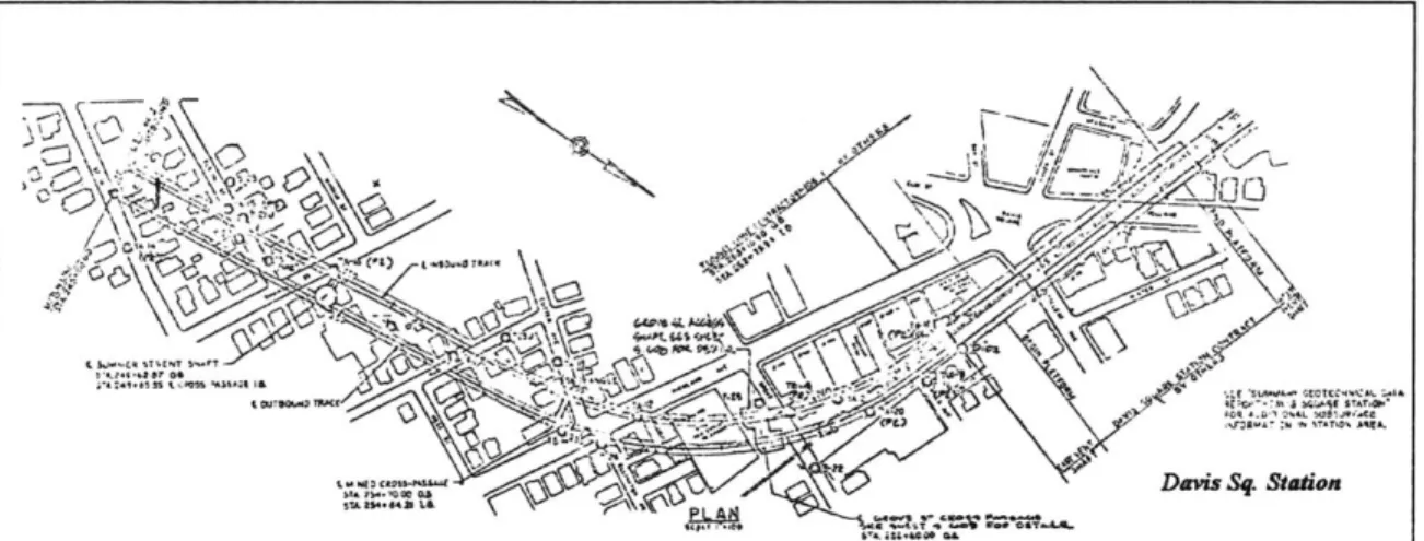
Figure 5.1a: Map of Porter Sq. to Davis Sq. alignment; Section of Porter Sq. 66
Figure 5.2: Borehole locations and alignment between Porter Sq. and Davis Sq. Figure 5.3: Borehole logs inserted into Nomad environment.
Figure 5.4 - Porter Sq.: Borehole information and geological profile. Figure 5.5 -Porter Sq.: Geological profile.
Figure 5.6a: Profile resulting from a coarse grid, (x-y-z)=(50-50-5) (ft). Figure 5.6b: Profile resulting from a medium grid, (x-y-z)=(5-5-5) (ft). Figure 5.6c: Profile resulting from a fine grid, (x-y-z)=(1-1-1) (ft)
Figure 5.7 - Porter Sq.: Experimental semi-variograms and exponential variogram models
Figure 5.8 - Porter Sq.: Experimental semi-variograms and spherical variogram models.
Figure 5.9: Geostatistical profile from kriging analysis based on an exponential model-Probability threshold 0%
Figure 5.10: Geostatistical profile from kriging analysis based on a spherical model-Probability threshold 0%
Figures 5.11 a: Kriged profile with probability threshold 30%. Figures 5.1 ib: Kriged profile with probability threshold 50%.
Figure 5.12: Semi-variogram models fitting the experimental data with small ranges.
Figure 5.13: Kriged profile with small range values-threshold 0%. Figure 6.1: General view of the site.
Figure 6.2: Plan view of the site. Figure 6.3: Profile along A-A.
Figure 6.4: Colored profile along A-A. Figure 6.5: Profile along B-B.
Figure 6.6: Colored profile along B-B. Figure 6.7: Profile along C-C.
Figure 6.8: Colored profile along C-C.
Figure 6.9: Experimental semi-variograms and semi-variogram models. Figure 6.10: Geostatistical profile along A-A - probability threshold 0% Figure 6.11: Geostatistical profile along A-A - probability threshold 35% Figure 6.12: Geostatistical profile along A-A - probability threshold 50%
Figure 6.13: Experimental semi-variograms and variogram models for profile B-B. Figure 6.14: Geostatistical profile along B-B - probability threshold 0%
Figure 6.15: Geostatistical profile along B-B - probability threshold 35% Figure 6.16: Geostatistical profile along B-B - probability threshold 50%
Figure 6.17: Experimental semi-variograms and variogram models for profile C-C. Figure 6.18: Geostatistical profile along C-C - probability threshold 0%
Figure 6.19: Geostatistical profile along C-C - probability threshold 35%
67 67 68 69 70 70 71 72 73 74 74 75 75 76 77 80 82 83 83 84 84 85 85 87 87 88 88 89 89 90 90 91 91 92
Figure 6.20: Geostatistical profile along C-C - probability threshold 50% 92
Figure 6.21: The 25 most frequently detected groundwater contaminants at
hazardous waste sites. 94
Figure 6.22: Sample representation of concentrations using NOMAD. 95
Figure 6.23: Acetone, 1993. 96 Figure 6.24: Acetone, 1996. 96 Figure 6.25: Arsenic, 1993. 97 Figure 6.26: Arsenic, 1996. 97 Figure 6.27: Benzene, 1993. 98 Figure 6.28: Benzene, 1996. 98 Figure 6.29: Toluene, 1993. 99 Figure 6.30: Toluene, 1996. 99
Figure 6.31: TCE plume prior to cleaning (April 1997). 100
Figure 6.32: Plan view of the wells monitoring Trichloroethane concentrations
during years 1997-2000. 102
Figure 6.33: Tabulated concentrations for Trichloroethane over time. 102 Figure 6.34: Concentrations for Trichloroethane over time at well locations. 103
Figure 6.35: Concentrations for Trichloroethane over time at well locations,
excluding the very high ones at ABB-15. 103
Figure 6.36: Trichloroethane, 1997. 105
Figure 6.37: Trichloroethane, February 1998. 105
Figure 6.38: Trichloroethane, April 1998. 106
Figure 6.39: Trichloroethane, May 1998. 106
Figure 6.40: Trichloroethane, July 1998. 107
Figure 6.41: Trichloroethane, September 1998. 107
Figure 6.42: Trichloroethane, 1999. 108
Figure 6.43: Trichloroethane, 2000. 108
Figure 6.44: Representation of TCE concentrations using the conventional contour
plot 109
Figure 6.45: True log(c) surface (unknown) and fitted surface. 111
Figure 1.1: Example of input spreadsheet. 124
Figure 1.2: Nomad menu options. 125
Figure 1.3: Nomad main window. 125
Figure 1.4: Shortcut buttons. 125
Figure 1.5: Explanation of shortcut buttons. 126
Figure 1.6: The Edit menu. 126
Figure 1.7: Example of a Ground types legend. 126
Figure 1.8: Nomad window with imported borehole data. 127
Figure 1.10: Model with curved lines.
Figure 111.1: Experimental semi-variograms and exponential semi-variogram models -coarse grid.
Figure 111.2: Kriged profile - exponential model - coarse grid - threshold 0%
Figure 111.3: Kriged profile - exponential model - coarse grid - threshold 30%
Figure III.4: Kriged profile - exponential model - coarse grid - threshold 50%
Figure 111.5: Experimental semi-variograms and exponential semi-variogram models -medium grid.
Figure 111.6: Kriged profile - exponential model - medium grid - threshold 0%
Figure 111.7: Kriged profile - exponential model - medium grid - threshold 30%
Figure 111.8: Kriged profile - exponential model - medium grid - threshold 50%
Figure 111.9: Experimental semi-variograms and exponential semi-variogram
models - fine grid.
Figure 111.10: Kriged profile -exponential model - fine grid - threshold 0%
Figure 111.11: Kriged profile - exponential model - fine grid - threshold 30%
Figure 111.12: Kriged profile -exponential model - fine grid - threshold 40%
Figure 111.13: Kriged profile - exponential model - fine grid - threshold 50%
Figure 111.14: Experimental semi-variograms and spherical semi-variogram models-medium grid.
Figure III. 15: Kriged profile -spherical model -medium grid - threshold 0%
Figure 111.16: Kriged profile -spherical model -medium grid - threshold 30%
Figure 111.17: Kriged profile -spherical model -medium grid - threshold 50%
Figure V.1: Principle of soil vapor extraction. Figure V.2: Examples of extraction wells.
Figure V.3: List of contaminants that can be cleaned up using soil vapor extraction.
Figure V.4: Principle of air sparging system.
128 139 140 140 141 141 142 142 143 143 144 144 145 145 146 146 147 147 175 176 176 177
Chapter 1: Introduction
The understanding and representation of the geological subsurface is the essential first step in all major projects in geotechnical and geoenvironmental engineering. Usually the information available for drawing geologic profiles is limited to data coming from boreholes (soil descriptions, SPT data, lithology, or RQD values, depending on the nature of the ground). Given a plan view of the site, alignments of cross sections are specified, and the boreholes, which fall within a certain distance from the alignment, are projected onto the vertical plane containing the alignment.
The procedure of geologic cross-section drawing used to be manual, but now computers are used to automatically create geologic profiles, based on the borehole data that has already been recorded in a spreadsheet. The main disadvantage of these methods is that programs usually do linear interpolation and the geologic judgement is in most cases ignored. Also programs do not often include options for updating the profiles according to changes in the given data, resulting for example from updated subsurface exploration or geologist beliefs.
In this context, geostatistics can provide more formal methods of visualizing the subsurface and they can furthermore offer means of evaluating where additional exploration should be carried out.
Indeed, geostatistics is widely accepted in the geologic, mining and engineering geology community, and it is believed that they should be part of the education of geologists, mining engineers, hydrogeologists and engineering geologists. Furthermore, construction people start realizing the significance of geostatistical profiles in reducing extra costs due to unexpected or misunderstood subsurface geology. However, one should be careful, since problematic results can occur if geostatistics are used without comprehending the concepts of the field, or without being able to recognize bad data.
Another important issue is that the three dimensional nature of the site is not usually extensively reflected. Boreholes are actually projected into 2-D planes and 2-D profiles are drawn. In order to reveal the three-dimensional nature of the site, cross sections in different directions can be drawn. The actual extrapolation into 3-D space depends on the
experience of the geologist or the engineer. Most importantly, the correct directions should be chosen. Furthermore one should simultaneously look at different profiles, critically compare them and remember the significant details. However, in practice, few cross sections are drawn and it is usually difficult to realize the 3-D nature of certain geological features.
Finally, problems of ground and groundwater contamination created the need to study the spatial distribution of pollutant plumes and, more importantly, their changes with time. Until recently only few programs were addressing this need. Moreover there was limited application of geostatistics to the representation of contaminant plumes.
In this context, a geostatistical program, NOMAD-KRIBS, was developed in earlier years at MIT in an effort to provide solutions for the above geological/geotechnical demands. Up to now, the program had not been used for hydroenvironmental data.
The present thesis is based on a research project that aimed at expanding the NOAMD-KRIBS software and at checking its suitability for hydroenvironmental (geoenvironmental) problems.
Specifically, the main objectives of the study were:
- to retain and improve the functionality of the software,
- to apply Nomad-KRIBS to geoenvironmental problems. As described above, these
problems, apart from having a 3D spatial nature, involve changes over time, which are of great interest in order to illustrate how pollutants advance and to predict their future distribution. The program, up to now, has been used for geologic cases that do not change with time, so its functionality for time dependent problems will be examined and it will possibly be adapted to other new demands.
Fulfillment of these objectives is presented with two case studies following an introduction to the program environment, to some geostatistical concepts and to previous research:
Chapter 2 presents the basic features of NOMAD-KRIBS, familiarizes the reader with the program's user interface and gives some details of KRIBS geostatistical algorithms.
Chapter 3 provides a review of the basic geostatistical concepts, emphasizing the main principles that were used to develop KRIBS. Among the topics discussed are Ordinary Kriging, variograms and variogram models, the handling of anisotropy, CoKriging, Block Kriging, and Bayesian Analysis.
Chapter 4 presents some previous research performed in geostatistics with main objective to review methods that KRIBS is using or could have used. In addition some new geostatistical concepts are presented and possible fields of future research are
discussed.
Chapter 5 reviews the MBTA Porter Sq. to Davis Sq. case study, that was used to check and improve the functionality of the program. Through this case study NOMAD features are presented in detail and decisions required in KRIBS modeling are discussed while comparing the different analysis outputs.
Chapter 6 presents the Wellesley Maintenance Depot case. Here the applicability of NOMAD-KRIBS to geoenvironmental problems, that involve the time parameter is studied and discussed. In parallel geological profiles are generated with NOMAD and compared with the ones statistically reproduced with KRIBS.
Chapter 7 summarizes the work presented in this thesis, discusses the conclusions derived throughout it and summarizes some future recommendations.
Chapter 2: NOMAD
-
KRIBS
2.1 Introduction
Nomad is a three-dimensional ground profiler using a combination of C, C++, XWindows and Motif on the Unix platform. It was originally developed at Massachusetts Institute of Technology by Noak (1988) [34] and extended by Kinnicutt (1991) [25]. On this graphical basis a geostatistical model, KRIBS, was later added by Kinnicutt (1995)
[27] in order to incorporate uncertainty in underground investigation programs.
Below, the basic features of NOMAD-KRIBS are presented. For more detailed information, description of the various features and for the manual of the program, one should refer to Kinnicutt 's Ph.D. Thesis [27], and also to Appendix I.
2.2 Nomad
NOMAD is a three-dimensional ground profiler. This means that spatial data about
the ground is stored as nodal information and can be recalled at any time. Cross sections in 2-D planes, usually used in project presentations, are not drawn using directly the borehole data, but they are resulting from the general 3-D profiler.
Input data are imported in .csv (comma separated values) format. Such a format can be exported from any spreadsheet program, which makes the manipulation of initial information easy and conventional. Figure 2.1 shows a spreadsheet containing the input data for a project. Each line in the spreadsheet contains attribute values (location, description, etc) for a certain borehole section. For each such line a NOMAD object, called a node, will be created in the program, and it will store all the above information. Each column is reserved for a different information category. The user can include ground types, SPT or RQD data, Atterberg limits or any other geotechnical information he believes is useful for distinguishing areas of uniform ground behavior, by just defining the category in the first row of that column.
File Edt Search View Forma Teoas _Op1ons Grapk Coenm s H*
D17] _
I
Figure 2.1: Spreadsheet containing input information for NOMAD
NOMAD reads from the imported data the spatial coordinates of all borehole points
for which information exists and illustrates them with colored intervals according to the corresponding ground type they define. Nodal data also stores all other information provided (SPT values etc). Figure 2.2 shows a general view of the program's interface with the imported borehole data. The three windows display the site from three orthogonally oriented directions. Each of the three views can be rotated, scaled and translated (Figure 2.3), either simultaneously or independently.
Dareb eas I x y_ desarpOa depN z Vieud type SPT R Q4OD v
-ABB-SB-1 80 860 6 Surface 0 100 Surface
ABB- SB- 1 580 060 B Widely graded 2 90 Widely graded sand 20
ABS- SB-i 880 060 8 Widely graded 4 96 Widely graded sand 24
ABS-SB- 1680 08 Widely graded 5 95 Widely graded Sand
ABS- SB-i 680 80 OSlr 7 5 32.58a
ABB-SB-i 680 8600 Widely graded 10 9 Widely graded sand
ABB-SB-1 680 860 8 Widely graded 12 68 Widely graded sand 30 ASOSB- 1 680 8 Widely graded 15 8 Wde Waded sand
AB- SB-1 680 060.8 Widely graded 152 84 8 Widely graded sand 20
ABB-SB-I 680 800Sot 164 93.6Si 20 ASS-SB-1 6 NO 80 O SS 20 B0SA
ABe-SB-1 60 NOBSe 22 7SSIR 20
ABB-SB-i 00 OM.8 SI 25 75 Sl 7
AMB-SB-2MW-1 1032 7104 Surface 0 100 Surface
ABS-SB-2VW-1 1032 7104 Widely graded 3 97 Widely graded sand 22
ADS-SB-2ftsW-1 1032 7104 Widely graded 3.5 98.5 Widely graded said 13 ADS-SB-2MW-1 1032 710A sandy SB 4 so sandy SO 13
AB-SB-2/MW-1 1032 710A sandy SIR 5 95 sandy SB
ABB-SB-20MW-1 1032 71OA sandy SIR 55 S 5 sandy S 221 ASS-Se-Z2MW-1 1032 7104 Widely graded 61 93.9 Widely graded and 22 AB-Se- /Mw-1 1032 710d Widely graded 10 90 Widely graded saNd
FWl Edie Oplisu View She Atrte Tnaabrm Ske Ambska Pr*ce Plot Wep
XZ=U ,YZ XY =-14. o; 2 r. 3MI)
Tnrivas L
EQk
ew
Lei~sess. SELECT NODE
Reaumber MMdleBuuem: KEYDOARD INPUT RightBumem: QUIT MODIFYING
_ .= .. k .. a.. -:.m.
Figure 2.2: General view of NOMAD interface
M1I Efte Op&.u ViewShe Asotiu Temfm=mShe Ambyuh Peejee Phi Help
ex XZ G.A YZuUA XY -1.s 0~-S 1Ae)
Tramdiennhd Lx Redraw Reste IJW. Precksioa Dmc Pwechim Dec. Preckebn
Reading SIT E datn hrvm &Wkatbemmked Vsratlaeiktemuple ex -o- ep FINISHED R EADING IN SIT ES
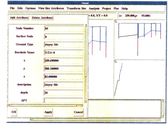
Once the input data are imported into NOMAD and a file is created, the user does not have to update the input file each time he wishes to make a change. The user can interactively edit the site data by inserting, deleting and moving nodal, borehole and line data according to his subjective beliefs or additional objective information. Figure 2.4 displays such an interface menu.
FRk Edk Optens View Se Atabutes Truander Su. Aml Pre nt PHi Kelp Add Actrbtel Dekeec Awrbute l
Node Nunba
j10
Ground Type
II;
B Trehul Name ZA-S
deqa
SPT
Figure 2.4: Edit menu that allows user to interact with the input data.
Lines and the layers they define are not generated automatically. This forces the user to use geologic judgement to introduce lenses or ignore information that seems to be affected by errors in investigation processes.
The user can also create cross sections and edit them, having the changes automatically propagated to the three-dimensional site model and to intersecting cross sections (Figure 2.5).
Sle Eit Optlew View teAtubuta Trionwarue Anab& Prject lot Hldp
SAMPLE M Z=3.X =3
F
i OU SU0AE
iddleButtew: KEYBOARD INPUT
Ii
1Rlgh1tbuen: QUIT MODIFYING Quit cW"e chamfg.d
k to sd. gravel
Figure 2.5: Cross sections can be edited, with the changes automatically propagated to the three-dimensional site model and to intersecting cross sections
2.3 KRIBS
2.3.1 Description of the program
KRIBS is a Kriging-Bayesian updating model for the creation of geologic profiles using Indicator CoKriging and Bayesian Updating techniques.
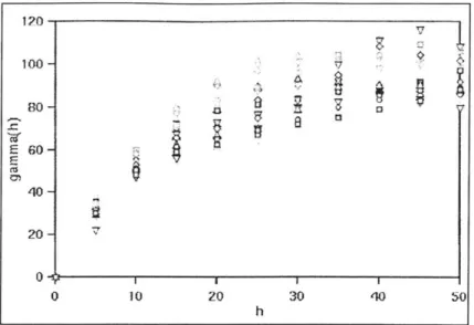
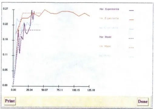
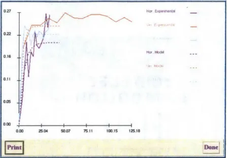
The KRIBS model can take into account the three-dimensional nature of the data as stored in the NOMAD files. For geostatistical analysis, the spatial structure of the data is captured with semi-variograms. The available semi-variogram models are the spherical, the exponential and the gaussian one. Because semi-variograms are constructed in 2-D planes, the actual kriging process is not three-dimensional. Figure 2.6 shows a set of experimental semi-variograms along with fitted models. Background information about the definition and modeling of variograms, along with reference to various geostatistical concepts can be found in Chapter 3.
Figure 2.6: Experimental semi-variograms andfitted models
The CoKriging feature allows the kriging model to consider two or more input data categories, such as both ground type information and SPT values, in calculating the probability of a ground type to exist in a certain location.
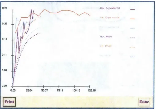
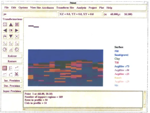
The program's output is a ground profile along with probabilities of each individual ground type occurring spatially in the profile and variances associated with each ground type. In other words, spatial uncertainties are captured. Figure 2.7 shows such a kriged profile. The user can choose a probability threshold when displaying the ground profile; in locations where ground types have been calculated to occur with a probability lower than the threshold the profile is blank, indicating that based on the criteria chosen, further site investigation should be carried out. Figure 2.8 shows the kriged profile with thresholds 25% and 50%. As the threshold increases, more areas are left blank; in those areas uncertainty is higher and further investigation may be required, depending on the significance of the project.
022 0.16 0.11 00 0.00 25.04 50.7 75.11 100.15 125.18 PrintDone 027 Hoe Ex ersnental
s View Sie Aitribates Transrm Ske Analysis Project Plot Help XZ .O., YZ =.0, XY 8.0 x: 6& .y 10.100) Fill Sandlgravel Clay TW Argillite >75 Argllite >50 Argillte <25
Figure 2.7. Kriged profile (from MBTA Porter Sq. case study).
u View SVe Artrbaoe Trmadsm Sif Amly* Peaee PIet He4
XZ I*. YZ 11A, XY U 0C QIUWJ lIA)
Fill
THI ArgUie >7S 1 --- Argivt >50
mum ArIIJhte <25
a View Ske Aurhaea Tram Skse Ambsky hsett Pet Hdp
)Cz-63.YZ =*XY-A (CAme.,IGA40
FWI Sand/gmvel Clay THI Arglike >73 Argll e <54 am~h~ .2
Figure 2.8: Kriged profiles with probability threshold 30% and 50%: Areas that appear blank correspond to ground types predicted to occur with probability less than
the threshold (from MBTA Porter Sq. case study).
Furthermore, the Bayesian updating features of KRIBS give the program the ability to incorporate additional objective and subjective knowledge in modeling a site. The kriged profile can be altered and probabilities of occurrence can be recalculated according to the geologist's beliefs or new objective information. Especially as far as personal beliefs are concerned, the user can develop subjective probability with a computerized probability wheel (Figure 2.9). The probability wheel makes use of the gaming theory. In this
"game", the user is given a choice (Fig. 2.9); either he can bet on the event that a certain ground type (sand) exists in a particular region, or bet that the roulette ball will fall in the blue region of the wheel (with the probability of the ball falling in this region being equal to the area of the region, assuming a total area of 1). User will place his/her bet on the game he is more likely to win; in other words one will bet on sand only when he believes that the probability of sand is greater than the area of the blue region. Until this happens, the user is presented with successive rounds of betting with different refined areas of blue region, so that to bracket his subjective belief that sand exists.
Figure 2.9: The probability wheel
function
enables user to input quantitativelysubjective beliefs (from Kinnicutt, 1995 [27]).
These features of KRIBS make NOMAD-KRIBS useful for locating the most suitable positions for new borings and planning efficient further exploration programs.
2.3.2 KRIBS algorithm
As described above, site data is organized into an input file, which is then read into
NOMAD and modified by the user. The KRIBS model is then initialized: Grid
dimensions are specified and the experimental semi-variograms, which capture the spatial
-r
configuration of the data, are calculated. Based on these experimental variograms, the user specifies the semi-variogram models to be used in the CoKriging system. Solution of this system provides the kriged profiles. Furthermore, information can be updated and the system solved again. The procedure is illustrated in Figure 2.10 below:
1 Collect Initial Data Set
2 Read into Nomad
lnitialize Data Matrix
Create 3-D Grid Translate Coordinates Populate Grid Calculate Experimental 4 Semi-variograms Specify Semi-variogram w 5 Model Create CoKriging Matrices Calculate Weighting I 6 Factors
Solve CoKriging System I Yes Finished? No Analyze Results 7 Update Information 8 Update? Yes No
--Figure 2.10: KRIBS algorithm (from Kinnicutt, 1995 [27]).
2.4 KRIBS model
Below some basic features of KRIBS model are cited for reference purposes. Geostatistical concepts are assumed to be known, but if this is not the case, one should refer to Chapter 3 and the corresponding bibliography.
Experimental semi variograms are calculated from the grided data in the x, y, z directions for up to 300/xiner step intervals, xincr being the grid increment in x direction.
The approximate horizontal distance for correlation between stratigraphic borehole data
3 1
has been found to be around 50 feet, therefore 300 ft was used in calculating the step intervals since this is twice the effective range for an exponential model'.
The equation for calculating the experimental semi-variograms in KRIBS is
1 N' 2
y(h,a) = - (z(x, + h)- z(x,)) (2.1)
2N' j=
where y(h,a) is the semi variogram for a distance h and a direction a,
N' is the number of data pairs encountered a distance h apart in direction a, z(xi+h) is the data value at location xj+h and
z(xd at location xi.
This equation corresponds to the mean of the variances of the differences between the experimental values and it assumes the intrinsic hypothesis, which states that the variogram function 2y(h,a) only depends on the distance and direction of (ha) and not on the location xi.
Currently, the KRIBS model calculates the experimental semi-variograms in the horizontal and vertical directions and also isotropically (all directions).
A lag angle of 22.5 is used to capture pairs of data, which are in the general direction of interest but are offset (Figure 2.11).
Area of consideration
Figure 2.11: Lag angle determining which pairs of data will be examined
See Chapter 3. Exponential model is defined in the bibliography either as y(h) =J-exp( -3h) or as a
- h
y(h)=-exp(--). KRIBS uses the latter case, so the effective range is 3a = 3*50ft =150ft. Twice the
a
The cone terminates into a band after reaching a specified bandwidth; this aims to minimize the effects of variances, due to spatial distances in direction other than the direction of interest.
Ideally experimental semi-variograms would be calculated for each ground type individually, then separate semi variogram models would be specified for each ground type, and different kriging systems would be created and solved. But such a procedure would require too much computational time. Instead, KRIBS specifies a model that captures how the ground types change with distance. Then, based on this one structural model, one kriging system is solved, and the same set of weighting factors are obtained and used for the estimation of the various ground types.
This model is able though of capturing the anisotropic properties in the soil by superimposing several different semi-variogram models, with each model capturing a particular component. More specifically, the semi-variogram model is of the form:
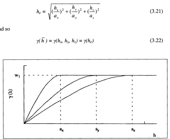
y(hx, h,, hz) = yodht) + yi(hi) + h2|+ y3dh3[) (2.2)
where y(hx, hy, h,) is the combined model and hi = ()2 +(h )2 +(h)2 , with ai
a a, az
accounting for anisotropy. Among the model components,
yo(]h[) captures the isotropic nugget effect (effect at small distances between data points)
yj(lh I) captures the horizontal behavior of the data - in this case az=O y2(1h2t) reflects zonal anisotropy in the vertical direction, so a,= ay =0
Chapter 3: Geostatistical concepts
3.1 Introduction
In this chapter some basic geostatistical concepts are presented. In more detail, this includes an introduction to Ordinary Kriging, and issues arising from the spatial description of a given data set, such as the definition and discussion of variograms and variogram models, and the handling of Anisotropy. Furthermore, CoKriging, Block Kriging, and Bayesian Analysis are briefly discussed.
The scope of this chapter is not to provide an exhaustive description of the geostatistical field, but rather to discuss the main principles that were used to develop KRIBS.
3.2 Ordinary Kriging
3.2.1. Introduction to Ordinary kriging
Ordinary Kriging is one of the Point Estimation methods that is also referred as Best Linear Unbiased Estimator (B.L.U.E.). It is considered linear because the estimates are weighted linear combinations of the available data, unbiased because it tries to have the mean residual (error) mR zero, and best, because among the other linear methods, it aims to minimize the variance of the errors qR2. The latter is actually the distinguishing feature
of the Ordinary Kriging.
In practice, the mean residual mR and the variance of errors UR2 are unknown. The best
approach one can make is to build a model and work with the average error and the average error variance for the model. In other words, to use a probability model in which the bias and error variance can both be calculated. Then, weights for the nearby samples are chosen so that the average error inR is exactly 0 and the modeled error variance
3.2.2. Main principle
At every point where no data exists, the unknown true value is estimated with a weighted linear combination of the available samples:
(3.1)
= 1w -v
j =1
where vj are the known values of the available samples
wj are the weights that need to be determined in order to obtain
-and v- is the estimation of the unknown true value. Note that the A symbol is used to denote the estimated values.
The weights are allowed to change as we estimate unknown values at different locations.
It can be proven (for example Isaaks, [17]) that in order to ensure unbiasedness, the sum of all the weighting factors should be 1:
n
j =1
(3.2)
This is the unbiasedness condition.
As mentioned above the main aim of ordinary kriging is the minimization of the
2 2
variance of the errors 6
R . '7R of a set of k estimates can be expressed as:
2 1k
UR =-I(ri -MR)
k j=1 (3.3)
With ri = i j- vi being the estimation error and
1=
r2 the mean residual error, (3.3) becomes:MR = -1r.thmenrsdaero,(.)bc e: k j=1 2i k 2 -- Y(^ -vi)] k j=1
Assuming that the mean error is 0, (3.4) is simplified:
2 1 k
OrR - i v 2
k
j=1(3.4)
Equation (3.5) gives an expression for 0
R2 but it is practically useless, since it requires
the knowledge of the true values vi. The probabilistic solution to this problem is to conceptualize the unknown values as the outcome of a random process and then to solve for the conceptual model. At any point where an unknown value is to be estimated, the model is a stationary random function consisting of n+1 random variables, n being the number of the existing data plus one for the unknown value that has to be estimated.
Introducing a random function model, the error variance can be expressed as:
n n n
2 -2WW 2 iij (3.6)
UR _ EE 1
i=1 j=1 i=1
where & 2 , C, are the random function model parameters (variance and covariance) and
wi are the n unknown variables (weighting factors). Note again that the ~ symbol is used to denote the model parameters
The minimization of a function of n variables is then accomplished by setting the n partial first derivatives to zero. So a system of n equations with n unknows is produced.
But since the unbiasedness condition (3.2) is also imposed, there is actually one more
equation in the system. Not any solution w1, ... wn of the nxn system satisfies the
unbiasedness condition and the problem is actually a constrained optimization with n+1 equations and n unknowns.
In order to convert the constrained system into an unconstrained one, the Lagrange Parameter technique is used. The Lagrange parameter p is introduced in the system as an extra unknown:
n n n n
2=- W W -2EwI, i-2i(Ew 1 (3.7)
i=1 j=1 ii=1
Equality is not violated since p is introduced in a term that is overall equal to zero. Furthermore, now by setting the n+1 partial first derivatives to 0 one gets n+1 equations,
The system in
C I
Cn
1
(n
matrix notation is:
C W= D
... C I (+ W1 C10
... Cnn I Wn CnO
1 0 P
-+ I)x(n -+1) (n+])xl (n+])xl
This is referred as the ordinary kriging system. The solution to it is
W = C~D
which gives the n values of the weighting factors plus i.
The minimized error variance is then calculated as
(3.9)
UR 2 2 2 - W -D
This is referred as the ordinary kriging variance.
In terms of the variogram, the ordinary kriging system can be written as:
(3.10)
wj fij- =fiO Vi=1,2, ... ,n.
j=1 n
j=1
and the modeled error variance n
UTR -jWiTO + A (3.11)
3.2.3. Comments
1. An important issue is how to take into account the spatial description of the data set. This will be discussed below in section 3.3
2. One should note C and D matrices require the calculation of the (n+1)2 covariances Ug and this is done by choosing a covariance function C (h) . Actually, what is fitted in the data values is usually the variogram model (section 3.3), then
C (h) = 7 (oo) - (h) (3.12)
with f (h) being the variogram model and Y (ox) its maximum value (sill).
3. The D matrix provides a weighting scheme similar to that of the various inverse
distance methods: the covariance between any sample and the estimated point generally decreases as the distance of the sample from the point increases. Actually the fact that D is formed by covariances makes it possible to consider not only geometric (or in other words physical) distances, but more generally statistical distances. The introduction of statistical distance takes into account both the physical position of the data values, and their spatial continuity. For example, consider two points 10m apart. Their physical or geometric distance is the same (10m), but they will have different correlation if the data concern the elevation of the groundwater table, rather than measuring gold concentration. The statistical distance in the latter case will have a much higher value, because groundwater elevation does not change significantly over a 10m distance, but gold concentration can exhibit very large fluctuations.
4. The C matrix records distances between samples, so it provides the system with information about the clustering of the sample data. Clustered values lead to large values in the C matrix whereas samples far apart result in small values at the corresponding matrix positions. Multiplying D with C-1 adjusts the distance (physical or statistical) weights of the D matrix to account for possible clustering of the sample
data.
Summarizing, the success of ordinary kriging is mainly based on the fact that it uses statistical distance instead of geometric distance and that it attempts to decluster the available sample data.
W= C-1 * D
3.3 Spatial description of a data set 3.3.1: Definitions
A powerful means of representing the spatial characteristics of a given set of data are
semi-variograms. A semi-variogram is defined as a means to summarize the information contained in an h-scatterplot.
An h-scatterplot is a plot showing all possible pairs of data values whose locations are separated by a certain distance in a particular direction (from Isaaks & Srivastava [17]). h=(O,1) means that each data location is paired with data location whose easting is the same and whose northing is 1 unit larger. h=(1,1) means that data are paired with the data location whose both easting and northing is 1 unit larger. This is illustrated in Figure 3.1:
(a) (b)
.
7
....
.+4
4- + ++++++ , 41* 4' 4 + 44
4
,))~4
/
7 1
4t '41 4(1
+/
Figure 3.1: Pairing of data to obtain an h-scatterplot: In the left figure each location is paired with the location being one unit further north than itself; in the right figure, each figure is paired with the location being one unit further north and one further east
than itself (from Isaaks & Srivastava [17]).
If there is no spatial variation, data values in both paired locations will be the same.
As spatial variability increases, the difference between the two values will increase. h-scatterplots are thus a cloud of points around the line y(x)=x. The shape of the cloud indicates how continuous the data values are over a certain distance in a particular
direction; if the data values at locations separated by h are very similar, the pairs will plot very close to y(x)=x. Otherwise, and as h represents greater distances, the cloud becomes more spread out and diffuses. This is illustrated in Figure 3.2.
Quantitative summaries of the information contained in an h-scatterplot (description of the cloud) can be done with:
-the correlation coefficient (which decreases as the cloud correlogram or correlation function plots the relationship coefficient of an h-scatterplot and h.
-the covariance, and respectively the covariance function -the moment of inertia of the cloud about the line y(x)=x.
(4)
of points spreads out). A between the correlation
(b) + +1 +* ++ + 44+ + rt+~ 7+ + + so 100 150 VQ) h (0.3) ++ + -4 4I'+ + + + (d (d) h h(0.2) Xl ++ ++ 7+ + + 7 + + 0 50 100 150 VMi 150 F h=(0.4) 100 Ar 50 f-1 0 ( 0 50 100 150 V() 4+ ++ + *+1 i++ + It + + I | 0 50 100 150 V(t)
Figure 3.2: h-scatterplots capturing spatial distribution of a variable V, for different values of h; as the pairing distance increases, data values become less correlated and the
cloud of points spreads out (from Isaaks & Srivastava [17]).
150 r h (0,j) 1001 2. t ! A
-F
0 (C) 50 0 - I 150 100, so k 0 ,I0 CConsidering that for h=(O,O), all points of the plot will fall exactly on y(x)=x (since each value will be paired with itself) and that as |h = h, + h, increases the points will
drift away from y(x)=x, this moment of inertia is a measure of how spread out the cloud is. Unlike the other 2 indices, the moment of inertia increases as the cloud drifts away.
The relationship between the moment of inertia of an h-scatter plot and h is called the semi-variogram (or simply variogram) of the data set.
Should Z( Z) be a random variable with I = [x,y,z], then the semi-variogram is defined through equation 3.13:
y(X-, X2) = Var [Z(X)- Z( X2)], (3.13)
where Var{] is the Variance of the random variable
Z( -) is the value of the random variable Z at location Ti = [xi, yi, z1]
y(zi, X2) is the variogram value for variable Z between the two locations X- and -2 3.3.2 Characteristic parameters of a semi-variogram:
As expected, in many cases, after a certain distance a the two random variables paired are no longer correlated. This distance is called the range of the semi-variogram.
At distances greater than a, the semi-variogram usually converges to a limit value known as the sill:
y(h> a) = y(oo) = s
Finally, at h = 0, the semi-variogram is defined to be 0; at small distances, however,
a discontinuity can exist in the variogram model. The behavior of the semi-variogram at those short distances is captured by what is called the nugget effect.
The above are illustrated in the Figure 3.3 below and a complete variogram surface is shown in Figure 3.4:
Y (h >= a) = s
y (h)
0
a Distance h
Figure 3.3: Sill s and Range a of a semi-variogram
Figure 3.4: Complete variogram surface. The depression at the center of the surface represents the variogram at zero distance (from Isaaks & Srivastava [17]).
3.3.3 Semi-variogram models
In geostatistical applications, a sample (or in other words experimental) variogram is calculated using the given data and then a function is fitted to it. This function models the spatial correlations for domains where there are no experimental data and provides a means of estimating the value of a random variable in regions where little or no data are known. A model has to be fitted and used instead of the sample variogram because:
1) A continuous relation is needed, since estimation could be required at any point in
space (and so the D matrix may call for variogram values for distances that are not available in the sample data).
2) The use of the sample variogram does not guarantee the existence and uniqueness of the solution to the ordinary kriging system. To guarantee that the system has one and
only one solution, and that this solution is stable, one must ensure that it possesses
the property of positive definiteness.
Actually, one should ensure that the matrix:
coo Co1.. COn
C= C10 CI .. C " (n+])x(n+l)
CnO C1 ... C
is positive definite.
A necessary and sufficient condition for this is:
wTCw > 0 =wiCov(ViVj ) >0 (3.14)
i=1 J=1
for any non zero vector w.
Taking into account that the variance of a random variable, defined by a weighted linear combination of other random variables, is given by:
Var{ wVL } = I E wiw1 Cov(1V1) (3.15)
i=1 i=1 j=1
if in (3.14) w is taken as the vector of weights, the positive definiteness guarantees that the variance of the estimation error,
n
Ro = wiVi -VO
i=1
In practice, (3.14) is not a useful way to check positive definiteness. For reference, other necessary and sufficient conditions are:
-All eigenvalues of C are positive.
-All submatrices of C have positive determinants.
-All the pivots (without row exchanges) are greater than 0.
In geostatistical applications, the positive definiteness is guaranteed by fitting in the experimental variogram a model (function) that is known to possess this property.
Several theoretical models have been developed using the hypothesis of stationarity' and positive definite properties. Variogram models can be divided into two basic categories: those that reach a plateau, and those which do not. The former are referred as transition models, the plateau is the sill, and the distance at which they reach the plateau is the range. Some models reach the sill asymptotically; in this case the range is defined as the distance at which 95% of the sill has been reached. Models, which reach no plateau, are representing cases where there is a trend or a drift in the data.
Some commonly used variogram models are the spherical, exponential, gaussian and linear ones:
Spherical model
y(h) = 41.5 -0.5(h ) , if h & a (3.16)
I if h>a
It is characterized by linear behavior at small separation distances near the origin, but flattens out at larger distances. It reaches the sill at range a and the tangent at origin intersects the sill at 2/3 of the range.
1 Stationarity: Stationarity is a concept of geostatistics according to which the covariance and
semi-variogram functions do not depend on the two data point locations in space, but rather only on the distance between the two data points. This assumption of stationarity is important in linear geostatistics, since statistical inferences can be made with many fewer data points (realizations of a random variable) than would otherwise be required. Different degrees of stationarity may exist, depending on the assumptions made.
Exponential model
y(h) = 1-exp(--3h (3.17)
It is linear at very short distances near the origin, but rises more steeply, and then flattens out more gradually. It reaches the sill asymptotically and the tangent at origin intersects the sill at about 1/5 of the range.
Gaussian model
3h2
y(h) = 1-exp(- 2
2 (3.18)
a2
It reaches the sill asymptotically. Its distinguishing factor is the parabolic behavior near the origin. Also it has an inflection point.
The three above-mentioned models are shown at Figure 3.5:
- - - exponential model
- - -- - Gaussian model
spherical model
range h
Figure 3.5: Relative plot of gaussian, exponential and spherical models.
The suitability of any one of these three models depends mainly on the behavior of the sample data near the origin. If the underlying phenomenon is quite continuous, pairs of data separated by small distances will have very similar values, so y(h) (which increases as correlation decreases) will have values very close to zero, or it will change at a very slow rate. This means that the tangent through the origin will be almost horizontal and therefore the sample variogram will probably show a parabolic behavior for small
distances. So, the Gaussian model will be the most appropriate. If the behavior near the origin is linear, which means that the data values have weaker correlation than in the parabolic case, even at small distances, a spherical or exponential should be tried. The choice between them depends on what part of the range a straight line drawn tangent near the origin intersects the sill, which again reflects how strong the correlation is at small distances. An exponential model, which has a steeper tangent at the origin, and intersects the sill at a smaller percentage of the range (20%), reflects much weaker correlations than the spherical one, which intersects the sill at 66% of the range. This can be understood when one bears in mind the definition of the variogram; the higher the value for a certain distance h, the more spread out the data points are, and thus less correlated (section
3.3.1). So, the steeper the slope in the variogram, the faster (in terms of increasing
distance h) the data become uncorrelated. In any case the physical explanation of the behavior should be examined.
Linear model:
y(h) = Ih (3.19)
It is obvious that it reaches no sill. As mentioned above, this models cases where there is a trend or a drift in the data set. As an example, one can think of mapping the elevation of a bedrock surface, when the bedrock is known to have a constant slope. Note that it is not always positive definite, but it can be if one insists that the weights sum to 0.
y(ho
y(h) = hi
h
Linear combination of models
The behavior of a sample data set can be modeled either using one basic model, or a linear combination of more than one of them. This is justified since positive definite variograms have the property that any linear combination of them is positive definite.
A final note would be that the distance h used in the semi-variogram models does not
have to be the physical distance between the points (h = x2+ y2+ z2 ), but can take
into account the geometrical anisotropies (different values in different directions), ax ay and az that the region may exhibit.
h = (ax)2 + (a, y)2 +(a, z)2 (3.20)
The physical distance can be used in the theoretical model if the ground is believed to be homogenous.
3.3.4 Effect of Variogram characteristics
a. Scale: The models have the same shape, but different sills. So correlation over distance does not change, but correlation at the same distance differs by a factor equal to the ratio of the two sills. (Figure 3.7). Thus scale does not affect the weights or the ordinary kriging estimate but only the ordinary kriging variance, which actually changes by the same factor that was used to rescale the variogram.
b. Shape: It affects how weights are distributed to the various data samples. For example
a parabolic behavior near the origin gives more weight to the closest samples. (Figure
3.8). Different shapes can result in negative weights or weights that are greater than 1.
This gives the procedure the advantage of being able to give estimates larger than the largest sample value or smaller than the smallest sample value. The disadvantage is that there exists the possibility of creating negative estimates (which should be set to zero). Nevertheless, even if the behavior seems to be parabolic near the origin, such models are avoided because negative weights make the estimation rather erratic.
![Figure 2.9: The probability wheel function enables user to input quantitatively subjective beliefs (from Kinnicutt, 1995 [27]).](https://thumb-eu.123doks.com/thumbv2/123doknet/14045360.459542/27.918.290.713.368.727/figure-probability-function-enables-quantitatively-subjective-beliefs-kinnicutt.webp)
![Figure 3.4: Complete variogram surface. The depression at the center of the surface represents the variogram at zero distance (from Isaaks & Srivastava [17]).](https://thumb-eu.123doks.com/thumbv2/123doknet/14045360.459542/40.918.295.657.420.701/figure-complete-variogram-depression-represents-variogram-distance-srivastava.webp)