Baroclinic instability of a meridionally varying basic state

1 .

BAROCLINIC INSTABILITY OF A MERIDIONALLY VARYING BASIC STATE

Stephen P. Meacham

B.A., University of Cambridge (1979) M.A., University of Cambridge (1983)

Submitted in Partial Fulfillment of the Requirements for the Degree of

Doctor of Philosophy at the

Massachusetts Institute of Technology and the

Woods Hole Oceanographic Institution June, 1984

Stephen Paul Meacham 1984

The author hereby grants to M.I.T. and W.H.O.I. permission to reproduce and to distribute copies of this thesis document either in whole or in

part.

Signature of Author

Certified by

Accepted by

Joint Program in Oceanography, Massachusetts Institute of Technology - Woods Hole Oceano-graphic Institution, June, 1984.

A, -

-Th73 siSpervi sor.

Chair n, oint Committee for hysical Ocean graphy, Massachusetts I titute of Technology - Woods Hole Oceanographic Institution.

MASE

ABSTRACT

The main topic is the finite amplitude evolution of weakly unstable, linear eigenmodes in a meridionally varying version of Phillips' two-layer model. Interactions between neutral modes and the

unstable mode strongly influence the evolution of the latter and are capable of stabilising it before significant changes occur in the zonally averaged flow. In the absence of resonant triad effects, the combined influence of changes to the mean flow and higher harmonics of the unstable wave is sufficient to equilibrate the unstable wave. The enhanced importance of neutral sidebands and the details of the evolution are interpreted as being consequences of the structure of the eigenmodes of the linear problem which is strongly affected by the meridional variation of the potential vorticity gradient of the basic flow.

Some aspects of resonant triad dynamics in a meridionally uniform, vertically sheared, two-layer model are also considered. Non-linear interactions between a resonant triplet of neutral waves can lead to baroclinic instability. Resonant interactions between a slightly supercritical unstable linear mode and two neutral waves can destabilise the weakly finite amplitude equilibration of the unstable mode that would occur in the absence of the sidebands, when the basic state is not close to minimum critical shear.

BAROCLINIC INSTABILITY OF A MERIDIONALLY VARYING BASIC STATE by

Stephen P. Meacham

Submitted to the Joint Commitee for Physical Oceanography of the Massachusetts Institute of Technology and the Woods Hole Oceanographic Institution, in June, 1984, in Partial Fulfillment of the Requirements for the Degree of

Doctor of Philosophy

ABSTRACT

Several problems are addressed herein. They are loosely connected

by the theme of resonant triad interactions. The main topic is the finite amplitude evolution of weakly unstable, linear eigenmodes in a meridionally varying version of Phillips' two-layer model. It is shown in chapter four that interactions between neutral modes and the unstable mode strongly influence the evolution of the latter and are capable of

stabilising it before significant changes occur in the zonally averaged flow. The evolution of the unstable wave in the absence of such resonant triad effects is also considered and it is shown by example that the combined influence of changes to the mean flow and higher harmonics of the unstable wave is sufficient to equilibrate the unstable wave. (The higher harmonics are unimportant in the meridionally uniform version of this model). The enhanced importance of neutral sidebands and the details of the evolution are interpreted as being consequences of the

chapter three that, near minimum critical shear, meridional variation of the potential vorticity gradient of the basic flow can introduce dramatic changes in the structure of the normal modes.

Some aspects of resonant triad dynamics in a meridionally uniform, vertically sheared, two-layer model are considered in chapter two. It is shown that non-linear interactions between a resonant triplet of neutral waves can lead to baroclinic instability. It is also demonstrated that

resonant interactions between a slightly supercritical unstable linear mode and two neutral waves can destabilise the weakly finite amplitude

equilibration of the unstable mode that would occur in the absence of the sidebands. This demonstration is limited to the case in which the basic state is not close to minimum critical shear. Finally, the work of Loesch (1974), who examined the evolution of a weakly unstable mode and a pair of neutral waves in a basic flow that is close to minimum critical shear, is repeated with the difference that critical layer effects are

included.

Thesis Supervisor: Joseph Pedlosky, Senior Scientist Department of Physical Oceanography Woods Hole Oceanographic Institution

ACKNOWLEDGEMENTS

I would like to take this opportunity to express my gratitude to my advisor, Joseph Pedlosky, who has been a steady and patient source of advice and encouragement since I first arrived in Woods Hole. I have benefited greatly from his perceptive criticism and the example of his

intellectual curiosity. The several people who have been associated with my thesis committee: Glenn Flierl, Peter Rhines, Paola Rizzoli, Mark Cane

and Erik Mollo-Christensen, have also been generous with their time and advice over the past few years.

My thanks go to Dale Haidvogel and Breck Owens for initiating me in the mysteries of spectral algorithms and vectorised FORTRAN. Thanks too to Bill Young, Bill Dewar and Bruce Cornuelle for suggesting the idea of enrolling in the Joint Program and for making it as much fun as they promised it would be.

During my time as a graduate student, I have had the good fortune to be in the company of a very stimulating and diverse group of people, namely the students and staff at both the Woods Hole Oceanographic Institution and M.I.T.'s Center for Meteorology and Physical Oceanography. Their contribution over the past four years to the life and work of this particular student has been large and I would like to make some acknowledgement of it here.

Large parts of this thesis could not have been completed without

the aid of computers. The computing staff of I.P.C. in Woods Hole and in

come to them with my pitiful tales of what the big, bad computer has done to me now. In particular, Karl Lindstrom, Cathy Sweet and Warren Sass deserve words of only the highest praise.

Just as indispensible to the preparation of this thesis has been the skillful typing of Anne-Marie Michael, who has shown an indefatigable good humour in the face of far too many equations.

The work in this thesis has been supported by the National Science Foundation under grant ATM 79-21431. In addition, part of the numerical work was performed on machines located at the National Center for Atmospheric Research at Boulder, Colorado. NCAR is funded by the

Contents Page Abstract 2 Acknowledgements 4 Contents 6 List of figures 9 0. Introduction 16 I. Background theory 27

II. Triad interactions in vertical shear flows

Abstract 44

Preliminary discussion 44

2.1 Non-modal baroclinic instability 47

2.1.1 Introduction 47

2.1.2 The evolution of a triad of neutral waves 50 2.1.3 A global stability constraint 64 2.1.4 Dynamics of a resonant triad in a

two-layer model 70

Energy balance 76

2.1.5 An example of an unstable triad 79 2.1.6 The range of unstable wavenumbers 81

2.1.7 Concluding remarks 86

2.2 Interactions between two neutral modes and a weakly unstable mode away from minimum critical

shear 88

2.2.2 Asymptotically unstable trajectories 100 2.2.3 Examples of triads exhibiting non-linear

instability 106

2.3 Three wave interactions near minimum critical

shear 116

Amplitude equations 118

Numerical solutions 128

III. Baroclinic instability in a meridionally varying

two-layer model: Linear theory 138

Model description 143

Numerical results 146

Eigenfunction structure 152

Heuristic expl anation of the meri dional structure

of 02 162

Analytical model 164

Energy balance 170

Neutral modes 173

Concluding remarks 176

IV. Baroclinic instability in a meridionally varying

two-layer model: Weakly non-linear theory 178

Asymptotic evolution equations 182

Energy balance for the finite amplitude system 208

Numerical results 213

The single-wave problem for the meridionally

8

Amplitude equations 240

Features of the asymptotic solution 254

Numerical simulations 259

The single-wave problem with the higher harmonics

excluded 267

V. Concluding remarks 270

Appendix A 275

Appendix B 276

List of Figures

Figure

1.1 (After Phillips, 1954, fig. 1) Contours of growth rate as a function of zonal wavelength L and vertical shear dU/dz , where L = 21/k and dU/dz = U*/H. The numbers on the contours indicate the doubling time (in days) of the gravest

unstable mode in Phillips' two-layer model. The parameters of the model were chosen so that:

H = 4.08 km , LD = 930 km , 8 = 1.6 X 10~11 m s~

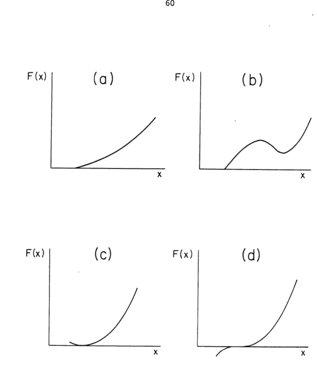
2.1 Possible forms of F(x) in the region to the right of the largest positive root, xj. In (a) and (b), F(x) intersects

1*

the x-axis at a finite angle. In (c) and (d), x, is a double or triple root.

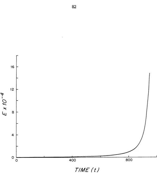
2.2 The evolution of the total perturbation energy of an unstable neutral wave triad over the interval 0 < T < 950. The triad is the one discussed in the text and the figure shows the results of a numerical integration of the potential vorticity equations.

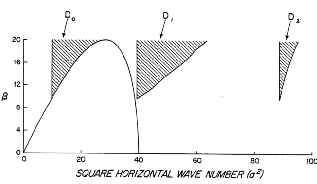
2.3 A map of the areas in the (8 , a2) plane in which may be found neutral Rossby waves that are elements of an unstable triad in which the waves have meridional structures given by n = (1,1,-2). The vertical structures of the three waves are assumed to be given by m = (-1,-1,1). Three regions are shown shaded, two of which overlap. Region Dj corresponds

2

to possible val ues of a.- Given a particular value of 8, for each choice of a. in D one can find a pair of

values (ak , a) lying in Dk X D1 ([j,k,1] = a cyclic permutation of [1,2,3]) which complete an unstable resonant triad. Note, for 8 < 12.95, there are no unstable

triads with this meridional and vertical structure.

2.4 A similar map to that in fig. 2.3, but with n = (1,2,3) and m

= ( -1, -1,1) .

2.5 a) Plots of M1, M2 and N0 as functions of s for a resonant triad consisting of two neutral modes and a marginal mode. The marginal mode corresponds to the left (long-wave) branch of the marginal curve. The meridional and vertical

structures of the triad are n = ( 1,-3,2) , mi = -1 , m2

= 1 (case A in the text) . b) KO as a function of a for the same triad as in fig. 2.5a.

2.6 a) As in fig. 2.5a but with neutral modes of different

vertical structures ( m, = 1 , m₂ = -1 : case B in the

text). b) K0 as a function of B for the same triad as in fig. 2.6a.

2.7 An example of the evolution of an unstable triad (case A, 8 = 13.0). The amplitudes of each of the three waves is shown. During the early part of the run (up to about T = 16) , the scale at the left applies. After about T = 16, the three curves are rescaled to accomodate their rapid growth and one should refer to the right-hand scale.

The evolution of a resonant triad near minimum critical shear. The triad consists of the marginal mode and two neutral waves. (a) - (d) show the evolution when the critical layer effect is excluded, (e) - (h) include this effect.

(a) and (e) (b) and (f) (c) and (g) (d) and (h) (F = 8, A0(0) = case 1) A 0 : AI A 2 P 1 .0707, A1(0) = .0177, A2(0) = 0.0; Similar Al(0) = Similar A1(0) = Similar A1(0) = to fig. 0.0354, to fig. 0.0707, to fig. 0.0146, 2.9 but A₂(0) ₌ 2.9 but A2(0) = for F 0.0354 for F 0.0707 2.9 but for F A2(0) = 0.0291 = 8, (case = 8, (case A₀(0) 2). A0( 0) 4). = 12, (case 9). A₀(0) = 0.0354, = 0.0354, = 0.582,

The tip of the numerically determined marginal curve plotted

in the (k2_{, s) pl ane.}

Case 1: F = 10.0, U = 1.0, h2 = 5.0 (sm = 15.0).

The full marginal curve for the gravest unstable mode of Case 1. 2.9 2.10 2.11 2.12 3.1 3.2

3.3 The real and imaginary parts of the phase speed, cr and ci, plotted against the square of the wavenumber. 8 = 14.96, A = 0.04 (F = 10.0, U = 1.0, h₂ = 5.0).

3.4 The phase speed along the right-hand branch of the marginal curve, c0(s), plotted against the supercriticality A.

(F = 10.0, U = 1.0, h2 = 5.0).

3.5 a) The magnitude of the lower layer streamfunction for the

unstable mode at B = 14.96, k = 2.261 (F = 10.0, U = 1.0,

h2 = 5.0).

b) The magnitude of the upper layer streamfunction.

c) Zonally averaged heat flux (multiplied by F) as a function of y.

3.6 The marginal curve for the gravest unstable mode when F = 6.6164, U = 1.0, h2 = 9.8836 (Case 2).

3.7 a) The magnitude of the lower layer streamfunction for the

unstable mode at s = 16.3 k = 2.544 (F = 6.6164, U = 1.0,

h2 = 9.8836).

b) The magnitude of the upper layer streamfunction.

c) Zonally averaged heat flux (multiplied by F) as a function of y.

3.8 Quantities associated wit the unstable eigenmode of fig. 3.7: a) heat flux, b) temperature tendency, c) upper layer momentum flux, d) lower 1 yer momentum flux, e) upper layer Reynolds' stress divergenc f) lower layer Reynolds' stress

divergence g) secondary circulation: upper layer meridional velocity h) secondary circulation: vertical velocity i) up-per mean zonal acceleration j) lower mean zonal acceleration.

Dispersion curves for the first three slow, neutral mode solutions of (3.26).

Kinetic energy of the (O)k Fourier component (wave 0) of the upper layer perturbation during run Al.

3.9

4.1

As fig. 4.1 but showing all components (waves 0-2).

three principal Fourier

As fig. 4.1 but during run Bl.

As fig. 4.2 but during run Bl.

wave 0, wave 1, - - - - wave 2.

Rates of baroclinic conversion of energy between an indivi-dual wave and the mean flow during Bl.

... wave 0 , wave 1, --- - wave 2.

Meridional profiles of the heat flux associated with the unstable wave, wave 0, at several times during run Bl. Profiles are plotted only for 0 < y < 0.5 , they are

symmetric about y = 0.5 . a) t = 0.0 , b) t = 4000.0 , c) t = 5500.0 , d) t = 11500.0, 4.2 4.3 4.4 4.5 4.6

e) t = 12500.0, f) t = 14500.0, g) t = 16500.0

4.7 The kinetic energy of the upper layer perturbation associated with wave 0 during several different runs. The initial amplitude of wave 0 was the same for each run. The values of F, U, a and h2 are the same as those used in run Al. The

wavenumbers and/or the initial sideband amplitudes differ between runs.

R22/24 is the first part of run B1.

R26: As R22/24 but with initial sideband amplitudes increased by a factor of 2.

R27: As R22/24 but with initial sideband amplitudes decreased by a factor of 2.

R31: Similar initial amplitudes as R22/24 but with ( k = 2.253, (lk = -1.2944, (2)k = -0.95858. Thi s corresponds

to a triad in which wave 0 has a smaller value of k

than in R22/24.

R32: Similar initial amplitudes as R22/24 but with 0 k = 2.267, (llk = -1.3008, (2)k = -0.96622. Here k2 is

2 larger than in R22/24.

4.8 As fig. 4.2 but during run A2.

4.9 As fig. 4.2 but during run B2.

4.10 As fig. 4.1 but during run A3.

As fig. 4.1 but during run B3.

CHAPTER 0

0. Introduction

The work in this thesis addresses some problems in the general area known as the theory of baroclinic instability. The purpose of this intro-ductory chapter is two-fold, to give a succinct statement of the problems dealt with in the remainder of the thesis and to provide a setting and motivation for those problems by briefly describing the phenomenon of baroclinic instability and some of the the techniques used to analyze it.

We will tackle the second objective first.

The main driving force behind the recognition and subsequent explora-tion of baroclinic instability has been the study of meteorology. It was recognized that, for a model Earth consisting of a rotating, spherical planet surrounded by a vertically, but stably, stratified atmosphere, a possible equilibrium response to the meridionally asymmetric net input of solar radiation was a steady, axisymmetric, convective circulation. To some extent this resembles the average properties of the tropospheric circulation. The mean winds are predominantly zonal and there is usually a large-scale meridional circulation in lower latitudes, the Hadley cell. However, there are many points of difference between the theoretical equi-librium circulation and the terrestrial troposphere. The real atmosphere is unsteady. Large, planetary scale waves may be seen standing or slowly propagating zonally in the height fields of the upper air pressure sur-faces. The equator-pole temperature difference on the Earth is substan-tially less than that predicted by the equilibrium model, suggesting a

meridional heat transport that is stronger than that associated with the meridional circulation of the equilibrium model.

It was shown by Charney (1947) that steady equilibrium flows like that of the model above tend to be unstable. Such a state contains a larger amount of potential energy than would a resting atmosphere in which the isopycnals lay parallel to the geopotential surfaces. The excess poten-tial energy is often referred to as available potenpoten-tial energy (Lorenz, 1967). Charney showed that there is a class of wave-like perturbations to such an equilibrium which can convert the potential energy of the equi-librium state to kinetic and potential energy of the wave. These waves can then grow at the expense of the equilibrium flow and are therefore known as baroclinically unstable perturbations. As the potential energy of the equilibrium flow is depleted, the isopycnal surfaces must become more nearly parallel to the geopotentials, i.e., the meridional tempera-ture gradient is reduced by the growing perturbations. As it grows, the unstable perturbation produces a meridional flux of density down the

horizontal density gradient, or equivalently, a meridional heat flux. Such an instability mechanism can go a considerable way toward explaining the existence of unsteady wave-like motions superposed on the general zonal circulation, the reduced equator-pole temperature differ-ence, and the reduced zonal velocities of the general circulation. Suf-ficient evidence seems to have been accumulated for it to be undeniable that the mechanism of baroclinic instability plays an important role in maintaining the average circulation of the Earth's troposphere. A descrip-tion of such a role in the context of a general circuladescrip-tion theory can

be found in the discussion by Charney (1959) of an idealized model atmosphere.

By dynamical analogy, there are some environments in the ocean which may support baroclinic instability by virtue of the available potential energy of the flow. These include vertically sheared boundary currents such as the Gulf Stream, open ocean currents such as the North Equatorial Current and the Antarctic Circumpolar Current, and broader areas of ver-tically sheared flow such as the recirculation regions adjoining the Gulf Stream and the Kuroshio. Direct evidence for the existence of baroclinic instability in the ocean is scantier than in the atmosphere and the role that baroclinic instability might play in the circulation of the ocean is less clear-cut. Since a down-gradient eddy heat flux is a symptom of a baroclinic conversion mechanism in the act of depleting the available potential energy of a larger scale flow, some investigators, notably

Bry-den (1979 and 1982) have looked for such fluxes as eviBry-dence of baroclinic instability. Bryden seems to have found such energy converting fluxes in

the Antarctic Circumpolar Current in the neighborhood of Drake Passage and in the Gulf Stream recirculation area.

The general circulation of the ocean is neither as well observed nor as well understood as that of the atmosphere, and one cannot say with certainty whether baroclinically active eddies are responsible for

sig-nificant meridional transports of heat across the main ocean basins. It is, however, known that the main ocean basins contain a substantial amount of energy at scales of the order of the internal deformation radius (e.g., Dantzler, 1977). In the interior of the subtropical gyres, this eddy

scale, slow, mean circulation. The question of what are the sources of this eddy activity is an intriguing one. One candidate for supplying part of this may be baroclinic instability of the stronger current and recirculation regions.

In recent years a considerable effort has been made to construct numerical models of the wind-driven circulation in idealized ocean

basins, that are capable of resolving eddies on the 100 km scale (e.g., Holland, 1978). These models, which have had some success in reproducing features such as western boundary currents that subsequently separate and the strong recirculation regions associated with them, also show the pro-duction of an active eddy field, some of which is converting available potential energy of the larger scale flow into eddy energy.

One _{last possible area in which baroclinic instability may be a} fea-ture is in the dynamics of the large rotating dust clouds that are pre-cursors of galaxies and galactic clusters.

Theoretical studies of baroclinic instability have had several goals: to elucidate the physical mechanism responsible for the instability, to discover which types of equilibrium state are unstable, to determine the distribution of the heat flux associated with the wave and to be able to describe how an initially small, unstable disturbance may evolve. Given the rather turbulent nature of the atmosphere and ocean, it is of inter-est to discover which horizontal scales are preferred by growing disturb-ances and how this energy is transferred to other scales to set up the observed energy spectra.

The usual starting point for theoretical investigations has been to take an equilibrium flow of simple forn, which satisfies the equation of motion; for example, a steady, uni-directional, non-divergent flow, and to study the evolution of small disturbances to this state by linearizing

the equations of motion about this equilibrium solution. The linear prob-lem can then be treated either as an initial value probprob-lem (Farrell, 1984; Pedlosky, 1964) or as a normal mode problem. Solutions in which the en-ergy of the perturbation increases with time are then classed as unstable. The philosophy behind such an approach is that if one starts with a very small perturbation to the equilibrium state, then the effects of the omit-ted non-linear terms will, at first, be small. The time scale for changes produced by the action of the non-linear terms will therefore be long. If the intrinsic properties of the linear solution are such that the en-ergy of that solution can increase on a finite time scale, then one can claim that the linear dynamics will give a good approximation to the

evo-lution of the unstable perturbation for as long as its energy is suffi-ciently small that the time scale of non-linear effects remains larger than the linear growth time scale. One expects that if the growth is sustained, then, after some initial period, the linear dynamics will become invalid and any consistent description of the subsequent evolution must also include non-linear effects. Several investigators have develop-ed techniques to follow the solution beyond the linear first phase.

Although the linear theory cannot tell us about the stability of an equilibrium flow to arbitrary disturbances of finite amplitude it appar-ently provides us with very useful information. It tells us something

turbations (more precisely, it tells us about the ability of flows to support instabilities which have a finite value for the initial growth rate in the limit that the initial amplitude of the perturbation tends to zero). It describes what spatial structures disturbances which belong to this class adopt. In some cases it tells us that a particular horizontal scale will grow more rapidly than others. It can even provide some idea of how a growing disturbance in this class will try to modify the equi-libri'um flow, if we calculate the quadratic fluxes of momentum and dens-ity that are associated with the growing disturbance by using the linear structure of that disturbance.

What linear theory fails to tell us about disturbances of weak initial amplitudes is whether there are types of small amplitude disturbance that do not possess any "linear" means of extracting energy from the equilib-rium state (in the sense that they do not contain an unstable normal mode of the linear system), yet nevertheless, by virtue of the non-linear terms in the equation of motion, can extract energy from that state. One would expect that any such disturbances would exhibit initial growth rates that are slower and slower as we make the initial amplitudes smaller and smal-ler (the linear limit). _{Yet is seems that from a physical point of view,} such disturbances might be important since in studying the stability of physical equilibria, one is concerned with stability to physical pertur-bations which will have a finite amplitude, even if this is small. A

second property that one might speculate upon for instabilities in which the energy extraction process depends on the non-linear rather than the

linear terms in the perturbation equations of motion, is whether the growth rate will not increase as the disturbance grows since the relative size of the non-linear terms, and hence the extraction rate, will increase as the square of the disturbance amplitude. Such an effect might make the instability of one of these weak, non-linear instabilities, whose development would be initially rather slow, ultimately rather powerful.

For the normal mode instabilities of linear theory, we have the unphysical result that the growing wave increases its amplitude at the same exponential rate forever and that no mechanism for diminishing the lack of stability of the underlying basic state is included. From the point of view of circulation modelling, one would like to know what changes the growing wave induces in the mean flow that is supporting the instability. One can obtain some insight into this by adopting a quasi-linear approach (Phillips, 1956; Charney, 1959). In this, the structure of the unstable wave is taken from linear theory, an amplitude for this wave is assigned or determined, the quadratic eddy fluxes are calculated and the resulting changes in the mean circulation are computed. Omitted in Phillips' theory is the feedback mechanism associated with the fact that, as the growing eddy field modifies the mean flow, so the insta-bility properties of the mean flow change and the growth characteristics of the eddy field are altered. If the modifications to the mean flow are such as to reduce its degree of instability, then the feedback loop is negative and one has a way of restraining the growth of the eddy field.

The fully non-linear problem which one would have to solve in order to follow the evolution of an unstable disturbance whose growth time scale according to linear theory was of the same order as the time scale

complicated. Charney (1959) simplified the problem by making the ad hoc assumption that the shape of the unstable Fourier component is unchanged by the non-linear interaction process. However, studies by Pedlosky (1970), Drazin (1970) and Pedlosky (1979) have shown that there is a class of non-linear evolution problems which are tractable. The technique that they exploit is to examine the evolution of a normal mode whose linear growth rates are slow in comparison to the advective time scale. Over much longer time scales, relatively weak non-linear interactions can compete with the linear instability. Non-linearity therefore becomes significant when the unstable wave is still small and one can develop a theory utiliz-ing perturbation methods, centered around the linear solution, in which the problem has two intrinsic time scales, the time scale of advection by the mean flow and the longer evolutionary time scale over which the disturbance amplitude changes. _{It is in this small amplitude limit that} Charney's shape assumption becomes justified.

By using such a "weakly finite amplitude" theory, one can explore the mechanisms by which non-linear effects curb the growth of an unstable disturbance once it reaches some sort of equilibrium amplitude (here and subsequently, the idea of an equilibrated amplitude will include the case of a state in which the disturbance amplitude fluctuates yet remains at a constant order of magnitude). This is not equivalent to a fully finite amplitude problem. If the tendency of a growing instability to push the mean flow towards stability persists into more strongly non-linear

re-gimes, then one might expect a natural tendency for an unstable flow to linger close to a stable state, i.e., be only moderately supercritical.

In such a situation, the degree of supercriticality would depend upon the forcing for the basic state and the dissipative mechanisms operating. This preference for a small degree of supercriticality would depend cruc-ially on the power of the wave-mean flow interaction mechanism. Stone (1978) has pointed to observations which suggested that the mean state of the troposphere is not too far removed from neutral, suggesting that weakly finite amplitude theories may be more relevant than just giving a mechanistic insight into the operation of non-linear processes.

Spectral transfers of energy must also be taken into account when deciding how a growing disturbance equilibrates. If the disturbance reaches an amplitude at which interactions between the unstable wave and neutral waves transport energy away from the unstable wavenumber at a rate comparable with that of the extraction of energy by the unstable wave, then the wave must eventually stop growing. For a statistically

steady state to develop by such a means, one again requires either dissi-pation at some range of space scales, for example, small scales, to mop up the cascade of energy ultimately released by the agency of baroclinic instability, or the modification of either the mean flow or the structure of the unstable and neutral wave modes in such a way that baroclinic en-ergy conversion is inhibited. An adequate model of the continuous spec-trum of waves that results from wave-wave interaction processes as a result of the baroclinic instability of a range of wavenumbers does not seem to have been developed. Instead, mechanistic models of how baro-clinic instability can couple to wave-wave interaction processes have been constructed, e.g., Loesch (1974).

The problem that I have attempted to address in this thesis is that 0 of the non-linear evolution of a weakly, baroclinically unstable wave when

the unstable equilibrium flow has a special type of meridional structure that makes the meridional potential vorticity gradient of the basic state exhibit a minimum within the channel. This sort of basic state has some of the features that a jet flow in a geophysical situation might exhibit and as such seems a worthwhile departure from the rather artificial merid-ionally uniform states studied by Phillips, Charney and Eady. A study of the linear problem, Chapter 3, shows that the presence of a potential vorticity gradient, of the form described above, imparts some distinctive features to the weakly unstable normal modes of the basic flow that are not observed in the meridionally uniform counterpart of this model. When one attempts to formulate the finite amplitude evolution of these weakly growing modes (Chapter 4), one discovers that the peculiar nature of the linear modes affects the way in which the finite amplitude evolution pro-ceeds. _{In particular, the effects of wave-wave interactions between the} unstable wave and neutral eigenmodes of the linear problem can exert a more powerful restraint on the growth of the unstable wave than the

alter-ation to the mean flow that the growing wave produces. Because of the prominent role played by wave-wave interactions in this non-linear model, some aspects of the interplay between wave-wave interactions and baro-clinic instability are explored in Chapter 2. In particular, we note

there that disturbances consisting of non-linearly interacting triads of neutral modes of the linear problem, with small amplitudes, can release potential energy from the equilibrium flow. These furnish an example of

a non-modal synopsis of subsequently

form of baroclinic instability. In Chapter 1, we present a some works whose content will be relevant to the research discussed.

1. Background Theory

In _{thi s chapter we will review some of the theoretical results} pre-sented in four papers which deal with material germane to the work of Chapters 2, _{3 and 4. These papers both serve as introductions to the} ideas exploited in the later chapters and furnish results with which the material of this thesis can be compared. The aim is not to present a comprehensive summary but to select some of the most pertinent details. At the same time we will introduce some of the notation that will be used later. The four papers in question are those of Phillips (1954), which looks at the linear theory of baroclinic instability in a meridionally uniform two-layer model; Pedlosky (1970), which looks at the finite amp-litude development of the slowly growing modes of Phillips' model; Longuet-Higgins and Gill (1967), which discusses resonantly interacting

triads of neutral waves in a barotropic model and of Loesch (1974) who examines the interaction of a growing baroclinic instability in Phillips' model with two neutral Rossby waves.

Phillips (1954) presents, as part of a theoretical study of the gen-eral circulation of the atmosphere, the properties of linearized pertur-bations to a quasigeostrophi c model of a zonal baroclinic jet. This idealized model allows only two degrees of freedom in the vertical by adopting a very coarse, finite-difference representation of the vertical structure. Such a model can be re-interpreted in terms of a system comprising two homogeneous layers of fluid, the second slightly more

dense than the first and lying beneath it. The two-layer and two-level models can be shown to be equivalent (Flierl, 1978), and in an earlier work Phillips (1951) chose a two-layer approach. Since the layer model can be realized physically and since the investigations of Pedlosky (1970) and Loesch (1974) were couched in terms of the two-layer model, we will adopted the layer formalism. Before continuing with Phillips' paper, we will pause to describe the model in the notation that will be used subsequently in this thesis.

The two layers of fluid are confined in a channel between rigid

boun-daries at latitude circles y = 0 and y = L, and heights z = 0 and z = 2H. This channel is assumed to be of infinite zonal extent and to be in a frame of reference which rotates with an angular velocity 1/2 f about a vertical axis. We desire to model geophysical flows whose width L is of the order of, but smaller than, the radius of the Earth. Following Rossby

(1939), we choose to include the dynamical influence of the Earth's spher-icity by using the s-plane approximation with f = f₀ + By. We are therefore constrained to working in mid-latitudes, where f0 is

signifi-cantly non-zero, and in a channel of limited meridional extent, such that Ls/f0 << 1.

We consider motions which have intrinsic and advective time scales that are long in comparison to the inertial period. Such motions include the traveling cyclone disturbances observed in the atmosphere and the synoptic scale eddying motions of the ocean. We adopt, as a filtering approximation, the quasigeostrophic approximation of Charney (1948). A detailed discussion of this and of the ancillary approximations that are used is given in Pedlosky (1979b).

The quasigeostrophic potential vorticity equations for the two-layer model of Phillips are

tD,2 g + (-1)j X2 (1 -2 + ,72 g + (-1)i x2 (01_ 02) + By] = 0

j

where our notation is closer to that of Loesch and Pedlosky than Phillips. pj f0

0j

jth

the upper layer, hence 0. is a streamfunction for the geostrophic flow in layer j. J is a Jacobian operator J(a,b)

=.

X2

f2

/

(gHA2-)

(1.2)

0 P1

where Ap is the density difference between the two layers. We have used

the Boussinesq approximation. In accordance with Phillips treatment, no bottom relief has been included and the interface between the two layers has been taken to lie at z = H when the fluid is quiescent, i.e., the lay-ers are of equal nominal depth, H. LD = x-1 is a dynamical length scale inherent to the system, often known as the internal deformation radius.

Following the several treatments of Pedlosky and others, we shall non-dimensionalize (1.1) at the outset. We do this by scaling: x and y with LR, z with 2H, t with LR/UR and 0 with URLR, where LR and UR are characteristic length and velocity scales of the motions of interest.

Equation (1.1) then becomes

at qj +

(Oj

In (1.3) and (1.4) #3 are scaled and dimensionless. q is the potential vorticity of fluid columns in the jth layer after the large but constant term f0 LR /UR has been subtracted. F and

I

given by B L2 _{R R}/U and is a ratio of the planetary vorticity gradient to the relative vorticity gradient of the fluid motions. We will make the assumption that, relative to the Rossby number, R = UR/(LR f0), both F and

a are 0(1). We will also drop the caret from '. It is convenient to use

a channel whose width is comparable to the horizontal scale of the motions of interest so we will set LR = L. The horizontal boundaries are there-fore located at y = 0 and y = 1 in this non-dimensional system. The phys-ical condition applied at the lateral boundaries is one of no normal flow which can be shown (Phillips, 1954) to imply that

# = 0 at y =0,1 (1.5a)

and

a af dx O. = 0 at y =0, 1 (1.5b)

where

dx

dx and we have assumed

f' L -+ 00

that # is uniformly bounded. Boundary conditions at z = 0 and z = 1 are not explicitly required, but they are implicit in the derivation of (1.1). We have used the condition of no normal flow through the horizontal boun-daries. Dissipative and direct forcing mechanisms have been excluded.

In particular, no Ekman layers have been included at the horizontal boundari es.

disturbances to a basic flow which consists of a uniform zonal velocity U. in each layer. In our notation, the linearized vorticity equations

for the perturbation are 0

(a + U a ) qj' + [s - (-1)j F (U -U2 j' = 0 (1.6)

Here the total streamfunction for each layer is decomposed into a basic flow plus a perturbation

# = - U y + #.'

and qj, is the potential vorticity of the perturbation. Phillips looks for normal mode solutions of the form

((1 ,2j) sin n iry exp [ik(x-ct)]

and finds that the phase speed, c, of these modes is given by

C =

T(a

_*[4

a2 F

- U

a

4

(4F

_{- a4]1/2}

₍₇

2a2(a1+2f) (

In this expression, a2 _{= k}2 _{+ n2 ,}2 _{is the total wavenumber of the the} perturbation, U = 1/2 (U1 + U2) is the mean velocity of the basic state

and Us = (U₁ - U2) is the vertical shear of the basic state in terms of the limited vertical resolution of the two-layer model. In general, there are two values of c for each wavenumber, a, corresponding to the two ver-tical modes possible in this system. The vertical structure of these modes is _{represented by the coefficient yj which is given by}

32

= a2 + F g + F Us

Yg gF U1- c(18

The system is insensitive to a uniform zonal translation of the reference frame so we may choose U2 = 0, U1 = U without any loss of generality, whence U = 1/2 U and Us = U.

The disturbance mode grows exponentially in time when c is complex with c

=

0 > arg (y.) > r/2

This phase lag between the upper and lower layer means that the heat flux associated with the perturbation, when averaged over a wavelength and integrated across the channel, i.e.,

1

k

r

_/k

dy 2-

dx T F

U (vI

v

)

(01-

2

0 0

is positive. It is this meridional transport of heat that is the mech-anism by which potential energy is released from the mean flow and con-verted into energy of the perturbation.

Phillips found that the contour-s of constant growth rate for the dis-turbance take the form shown in Figure 1.1. In Figure 1.1, the contours of constant growth rate are mapped on a plane with axes corresponding to the basic shear and the disturbance wavelength. There are several

fea-6

0.75

5

1.5

2

3-

2-0

0

2

4

6

8

10

12

14

L

--

(0

3

_km)

Figure 1.1: (After Phillips, 1954, Fig. 1) Contours of growth rate as

a function of zonal wavelength L and vertical shear dU/dz , where L =

2w/k₀ and dU/dz = U*/H. The numbers on the contours indicate the doubling time (in days) of the gravest unstable mode in Phillips' two-layer model. The parameters of the model were chosen so that:

s-34

tures of this graph which we wish to note for future reference. There i s a minimum critical shear below which baroclinic instability is not possi-ble. This is also the value of the shear parameter above which the two-layer model version of the sufficient criterion for stability derived by Charney and Stern (1962) is no longer satisfied. If one rearranges the dispersion relation, one can show that the boundary between neutral and unstable perturbations is determined by only two parameters a/FU and a2/F. Thus for fixed F, increasing U is equivalent, as far as stabil-ity properties are concerned, to decreasing s. Thus, if we view F and U as fixed, the stability threshold noted above corresponds to a minimum critical B above which instability is not possible. In subsequent chap-ters, this is the view which we will adopt. This should not be allowed to obscure the fact that what we are really doing is varying the dynam-ically significant parameter a/FU which, in the dimensional variables, is

s* 2

rrLD

The asterisks are to denote true dimensional quantities and LD is the internal deformation radius defined earlier. The stability threshold amounts to requiring that the vertical shear Us* exceed a value deter-mined by the strength of the restoring force for vorticity oscillations, represented by a* and the inertia of the system to internal oscillations represented by LD'

For values of the shear above the critical threshold only a limited range of wavenumbers is unstable; both a long and a short wave cutoff are

stability boundary in Figure 1.1) is parabolic. The growth rate tends to zero as one approaches the stability boundary, i.e., the modes close to the marginal curve grow only slowly with time.

Using the analytically determined forms of the linear eigenmodes, Phillips went on to compute the eddy heat flux associated with the unstable mode and thence the secondary meridional circulation and the changes to the mean zonal flow that these fluxes would have produced after a certain time had elapsed. Phillips' aim in using this quasilinear theory was to estimate the redistribution of heat and momentum that the baroclinic eddies might produce when they had grown to amplitudes that might be typical of the Earth's atmosphere. Because such a theory does not include any feedback between the changes induced in the mean flow by the growing waves and the instability properties of the waves, the choice of wave amplitude used in such a calculation is, in a sense, arbitrary. Phillips chose the wave amplitude by requiring that the rate at which the heat transported by the eddies warmed the northern half of the "northern hemisphere", that his model represented, match the estimated diabatic cooling rate for the same region. Phillips provided a rather successful theoretical model of some of the qualitative effects of eddies on the mean circulation that had been postulated by Jeffreys (1926, 1933). But this model still leaves unclear the answer to the question of how the growth of the unstable eddies is curtailed. However, the seeds of a pos-sible mechanism are contained within this model. The alteration to the mean flow calculated by Phillips as a consequence of the growing waves

was such as to reduce the average vertical shear of the mean flow. The linear results indicated that the mean flow was less unstable (the growth rates at a given wavenumber were less) at smaller shears, so that this second order effect should be stabilizing. The non-linear analysis required to incorporate this feedback mechanism in the general case of initial parameters that corresponded to an unstable wave whose growth rate was 0(1) seems rather intractable. Charney later refined Phillips' model (Charney, 1959) and included this stabilizing mechanism in a heur-istic way by balancing the rate at which energy was released from the modified mean flow against the rate at which perturbation energy is

dis-sipated. Pedlosky (1970) recognized that under some circumstances, the non-linear analysis could be simplified and this feedback mechanism

successfully included in a more rigorous fashion.

The essence of Pedlosky's method is to look at a single unstable wave whose growth rate is small because one has chosen values of B/FU and

a2/F that lie close to the position of the marginal curve. We shall describe the case for which s/FU does not correspond to the position of minimum critical shear but rather a2/F and s/FU are such that the point

they define on a stability diagram such as Figure 1.1 lies near to one side of the marginal curve. The original basic flow is then only slightly unstable for a disturbance at the wavenumber described. As the initially linear unstable eigenmode grows, it produces a correction to the mean flow that is proportional to the square of the eigenmode amplitude. This re-duces the mean vertical shear. However, since the original mean flow was only slightly unstable, only a relatively small modification is required

weak, it has succeeded in choking the mechanism that was allowing it to grow. The fact that throughout this process the unstable wave has never reached a large amplitude enables one to develop the non-linear solution as a perturbation series in the amplitude of the unstable wave or, more conveniently, in the distance below the marginal curve that the initial

value of s/FU lies, since it is this that controls the amplitude that the unstable wave can reach.

The above is a rather sketchy summary of the basic mechanism operat-ing in the non-linear model considered by Pedlosky. The detailed picture

is somewhat more involved and one should refer to the paper in question for the precise nature of the evolution. Pedlosky's analysis shows that the growth of the unstable wave is halted by the mean flow modifications and that, in the absence of friction, the amplitude of the unstable wave vacillates in a regular, periodic way. Because the parameters are such that the unstable wave lies close to the marginal wave, the e-folding time scale of the linear unstable eigenmode is long in comparison to the periods of most of the neutral waves. This fact is used in the method of

analysis, which considers separating the dynamics that occur on the two time scales. The amplitude vacillations of the unstable wave are

charac-terized by the longer, e-folding time scale.

In choosing to site this weakly finite amplitude analysis close to the side of the marginal curve rather than in the vicinity of minimum critical shear, one is including an element of inconsistency in that, for the same value of a/FU, there are wavenumbers further into the interior of the unstable region which have larger, 0(1), growth rates that would

overpower the unstable wave on which the analysis has been concentrated, and to which the weakly finite amplitude analysis would be inapplicable. One situation in which this might be avoided would the case of a periodic zonal domain such as an annular channel in which the quantization was such that the only unstable wave which fit the domain was one close to the marginal curve.

One would prefer to look at an unstable mode in the vicinity of mini-mum critical shear. For the meridionally uniform model, the finite amp-litude problem in the neighborhood of minimum critical shear is a little degenerate and one finds a critical layer effect which alters the behav-ior of the problem (Pedlosky, 1982). Alterations to the mean flow can cause the unstable wave to equilibrate but the finite amplitude evolution is more complicated than a periodic amplitude vacillation and many zonal scales are stimulated (Pedlosky, 1982; Boville, 1981). The inclusion of meridional variation in the potential vorticity gradient or velocity

field of the lower layer should remove this effect.

It may at first seem something of a limitation to confine attention only to the weakly growing waves near the marginal curve, however, this

is not so strong a constraint as it might appear. The weakly supercriti-cal waves are those which one first encounters as one gradually increases

the mean shear to pass from the stable regime to the unstable regime. If the tendency of a growing baroclinic disturbance to stabilize the verti-cal shear is robust, as the work of Phillips would suggest, then one has a dynamical reason for the mean flow to lie not too far from critically stable conditions.

anism for curbing the growth of a baroclinic instability that linear theory alone would not have predicted and shown how this pivots on the way in which the growing wave modifies the mean flow. One of the reasons for being interested in the dynamics of finite amplitude eddies was their ability to transport heat. In the equilibrated inviscid model of Ped-losky (1970), the mean meridional eddy heat flux, when averaged over a vacillation period, is zero' However, the introduction of dissipation (e..g., Pedlosky, 1971) enables one to recover a non-zero average heat flux in a model which retains the wave-mean flow interaction process as a method of containing the growth of an unstable perturbation.

The model described above does not include any interaction between the unstable wave and neutral waves of the system. The inclusion of non-linear processes allows the possibility of such interactions. Pedlosky's model is consistent in that, given initial conditions in which neutral Rossby waves are absent, they will not, in general, be forced by the dynamics of the unstable wave at amplitudes that would be significant. However, if such waves are included in the initial conditions, alongside the unstable wave, it is possible under some circumstances that they will interact with the unstable wave on the time scale of the weakly finite amplitude evolution theory.

Such wave-wave interactions (as distinct from the wave-mean flow interactions present in Pedlosky's model) may be of interest for several reasons. They may, for example, allow the energy extracted from the mean flow by the primary baroclinic instability to be transported to other

length scales that are not directly unstable. There may be significant transport of energy to shorter, more dissipative length scales. Such an effect might alter the size of the heat flux associated with the unstable wave in an "equilibrated" state. The forcing of neutral waves having amplitudes comparable to the unstable wave and fluctuating on the same timescale as the unstable wave would produce additional modifications to the mean flow of similar size to that produced by the unstable wave and so modify the equilibration process described by Pedlosky (1970).

A general attempt to model interactions between a range of unstable waves and a spectrum of neutral waves would be extremely complicated. However, models which included only one unstable zonal Fourier component and a small number of neutral Rossby modes would be more manageable and should give some insight into the interplay between wave and wave-mean flow interactions. An attempt to construct such a model has been

made by Loesch (1974). Amongst waves of weak amplitude it can be shown that the strongest wave-wave interactions occur between waves which form certain resonant multiplets. For the particular dispersive properties of the eigenmodes of the two-layer model, the appropriate multiplets are triplets. Before discussing Loesch's paper, it will be useful to briefly consider the dynamics of resonant triads. These are discussed, albeit for a different physical system, by Longuet-Higgins and Gill (1967).

Longuet-Higgins and Gill considered interactions between Rossby waves in an equivalent barotropic model on an infinite a-plane in which there was no mean flow. Such waves interact most readily when three of the waves satisfy resonance conditions similar to

j=1 ~ 3 '_

where k are the horizontal wavenumbers of the three waves and a. (k.) are the frequencies. In the above paper, equations governing the slow evolu-tion of the amplitudes of three waves, satisfying these resonance condi-tions, are obtained for the case in which each of the waves is of small amplitude. If E, << 1, is a small number characterizing the amplitudes of the three waves, then the non-linear interactions between the elements of the resonant triad modify the amplitudes on a time scale, e~1. The evolution, in general, takes the form of a phase locked vacillation in the amplitudes of the three waves, where the relative phases are such that the energy of the triad as a whole remains constant. When the three waves satisfy a further constraint on their relative phases, Longuet-Higgins and Gill show that the amplitudes of the three waves may be described by Jacobian elliptic functions. It can be shown that this is also true for general relative phases of the waves. The authors also showed that in the case of the single layer model without any mean flow, the triad must conserve its total wave energy. They also calculated the amplitude of one of the waves non-resonantly forced by the non-linear interaction and showed that the small amplitude dynamics are consistent when the ratio of particle velocity to phase speed is small for each of the three principal waves.

The importance of this triad interaction phenomenon is that it indi-cates a preferred mechanism for the transfer of energy between wavenum-bers in a weak wave-field. Each element of the triad would, in a more

realistic system, be involved simultaneously in triad interaction with other neutral modes. In a situation in which energy is being injected slowly and over a limited range of wavenumbers, one might expect that resonant triad interactions, at least initially, will be important in redistributing this energy over the wavenumber spectrum. If there is sufficient dissipation to allow an equilibrium spectrum of weak energy to be established, then triad interaction will continue to be important. Such a slow injection of energy at a narrow band of spatial scales could be the result of baroclinic instability under weakly supercritical conditions.

Loesch (1974) considered a model in which a single baroclinically unstable wave, in a flow similar to that considered by Phillips (1954), was allowed to interact resonantly with a pair of neutral Rossby waves. The unstable wave was presumed to lie a small distance A below the mar-ginal curve so that in the absence of the neutral waves it would evolve according to the weakly finite amplitude theory of Pedlosky (1970, 1982). The two neutral waves were chosen to form a resonant triad with the mar-ginal wave adjacent to the unstable wave. Loesch showed that when the unstable wave was near one of the sides of the marginal curve, i.e., away

from minimum critical shear, the dynamics of both the wave-mean flow interaction process and the resonant triad interaction would be signifi-cant (i.e., the time scales of changes in the amplitude of the unstable wave to wave-mean flow interaction and in the amplitudes of all three waves due to wave-wave interactions between the triad elements, are

instabil-ity) when the amplitude of the unstable wave is 0(1A1112), where A is the supercriticality, and the amplitudes of the sidebands are O(jA13/4_).

Loesch did not consider this case any further and moved on to the case in which the slightly supercritical mode lies just below minimum critical shear, showing that again the processes of wave-mean flow interaction and triad interaction could be equally significant. In this instance, the natural scales for the wave amplitudes are each 0(1A112

The two features of such a system are firstly that the energy of the

"unstable" _{mode is shared with waves whose length scales are stable}

according to linear theory and secondly that the finite amplitude evolu-tion of the unstable wave is modified by the presence of the sidebands. However, we emphasize that the wave-mean flow interaction mechanism nev-ertheless remains an integral part of this evolution. This should be contrasted with the results that will be presented in Chapter 4. The numerical computations of Loesch did not allow for the critical layer effect noted by Pedlosky (1982) so we will not discuss their results here, but the discussion of amplitude scaling and hence the relative importance of the two non-linear interaction mechanisms remains valid.

CHAPTER 2

2. Triad Interactions in Vertical Shear Flows

Abstract

Three related problems concerning the evolution of disturbances in Phillips' model are considered. Firstly, it is shown that non-linear interactions between a resonant triplet of neutral waves in a vertically sheared flow can lead to baroclinic instability. Secondly, we demonstrate that resonant interactions between a slightly supercritical unstable linear mode and two neutral waves can destabilize the weakly finite amplitude equilibration of the unstable mode that would occur in the absence of the sidebands. This demonstration is limited to the case in which the basic state is not close to minimum critical shear. Thirdly, we repeat the work of Loesch (1974) in examining the evolution of a weakly unstable mode and a pair of neutral waves in a basic flow that is close to minimum critical shear with the difference that critical layer effects are included.

A feature of the finite amplitude analysis to be presented in

Chap-ter 4 will be the inclusion of wave-wave inChap-teractions between members of a resonant triad. It became clear while studying this material that there were some interesting differences between resonant triad interac-tions in a shear flow and their counterparts in a fluid at rest. For that reason, we have included the brief studies that make up this chapter.