Publisher’s version / Version de l'éditeur:
Atmospheric & Chemical Physics, 6, 8, pp. 2231-2240, 2006-06-21
READ THESE TERMS AND CONDITIONS CAREFULLY BEFORE USING THIS WEBSITE.
https://nrc-publications.canada.ca/eng/copyright
Vous avez des questions? Nous pouvons vous aider. Pour communiquer directement avec un auteur, consultez la première page de la revue dans laquelle son article a été publié afin de trouver ses coordonnées. Si vous n’arrivez pas à les repérer, communiquez avec nous à PublicationsArchive-ArchivesPublications@nrc-cnrc.gc.ca.
Questions? Contact the NRC Publications Archive team at
PublicationsArchive-ArchivesPublications@nrc-cnrc.gc.ca. If you wish to email the authors directly, please see the first page of the publication for their contact information.
NRC Publications Archive
Archives des publications du CNRC
This publication could be one of several versions: author’s original, accepted manuscript or the publisher’s version. / La version de cette publication peut être l’une des suivantes : la version prépublication de l’auteur, la version acceptée du manuscrit ou la version de l’éditeur.
For the publisher’s version, please access the DOI link below./ Pour consulter la version de l’éditeur, utilisez le lien DOI ci-dessous.
https://doi.org/10.5194/acp-6-2231-2006
Access and use of this website and the material on it are subject to the Terms and Conditions set forth at
Detection and measurement of total ozone from stellar spectra: Paper
2. Historic data from 1935-1942
Griffin, R. E. M.
https://publications-cnrc.canada.ca/fra/droits
L’accès à ce site Web et l’utilisation de son contenu sont assujettis aux conditions présentées dans le site
LISEZ CES CONDITIONS ATTENTIVEMENT AVANT D’UTILISER CE SITE WEB.
NRC Publications Record / Notice d'Archives des publications de CNRC:
https://nrc-publications.canada.ca/eng/view/object/?id=11c7ee39-05b0-4aa6-b279-2cb6580dc9b9
https://publications-cnrc.canada.ca/fra/voir/objet/?id=11c7ee39-05b0-4aa6-b279-2cb6580dc9b9
Atmos. Chem. Phys., 6, 2231–2240, 2006 www.atmos-chem-phys.net/6/2231/2006/ © Author(s) 2006. This work is licensed under a Creative Commons License.
Atmospheric
Chemistry
and Physics
Detection and measurement of total ozone from stellar spectra:
Paper 2. Historic data from 1935–1942
R. E. M. Griffin
Department of Earth and Space Sciences and Engineering, York University, 4700 Keele Street, Toronto, ON, M3J 1P3, Canada, and Herzberg Institute for Astrophysics, 5071 West Saanich Road, Victoria, BC, V9E 2E7, Canada
Received: 22 July 2005 – Published in Atmos. Chem. Phys. Discuss.: 31 October 2005 Revised: 3 March 2006 – Accepted: 24 April 2006 – Published: 21 June 2006
Abstract. Atmospheric ozone columns are derived from historic stellar spectra observed between 1935 and 1942 at Mount Wilson Observatory, California. Comparisons with contemporary measurements in the Arosa database show a generally close correspondence, while a similar comparison with more sparse data from Table Mountain reveals a differ-ence of ∼15–20%, as has also been found by other researches of the latter data. The results of the analysis indicate that as-tronomy’s archives command considerable potential for in-vestigating the natural levels of ozone and its variability dur-ing the decades prior to anthropogenic interference.
1 Introduction
Studies of the changes in the distribution and concentration of ozone (O3) in the stratosphere detected in the latter half
of the 20th century reveal patterns that could presage sig-nificant alterations in the protection which the O3layer has
provided to living organisms on the surface of the Earth. The cause of the changes is widely attributed to anthropogenic interference; historical evidence, though somewhat limited, indicates a general correlation between a major increase in the industrial use of CFCs and their indiscriminate release into the atmosphere, and a decrease in O3 columns. Some
of the measured changes may also have had natural causes, but it is not easy to establish how much; despite a consid-erable interest in stratospheric O3, particularly in Europe, in
the early 20th century, only one site – Arosa, in Switzerland – has maintained (since 1926) a long, continuous series of O3measurements of acceptable quality. There is a clear need
to exploit all other possible resources for measurements of total O3. One such unexploited resource is the world’s
her-itage of stellar spectra.
Correspondence to:R. E. M. Griffin (elizabeth.griffin@nrc.gc.ca)
All ground-based stellar observations of the appropriate wavelength region bear signatures of O3which can be
mea-sured and interpreted in terms of total column O3.
Deter-minations of O3 columns from measurements of the
Hug-gins bands (∼λ 300–335 nm) made on stellar spectra ob-served relatively recently (1978–1992) were shown by Grif-fin (2005; hereinafter Paper 1) to compare satisfactorily with simultaneous TOMS1 measurements, and a small selection
of considerably older stellar spectra is now being investigated by the same techniques. This paper presents some of the re-sults; Sect. 2 outlines the archive searches and Sect. 3 the data digitization and spectrum extraction. Section 4 describes the measurements of O3features, their principal sources of
un-certainty, and their conversion into O3columns, corrected to
zenithal air-mass. Section 5 then compares those results with values for the corresponding dates in two solar databases.
2 Resources of historic stellar spectra
2.1 Spectroscopic archives
From the beginning of the 20th century until well into the 1970s or later when it was gradually replaced by electronic devices, the photographic plate was the workhorse detector for observational astronomy. Nearly all of astronomy’s spec-troscopic plates have been preserved and are in relatively safe keeping (though not infrequently in conditions that may hasten their eventual deterioration), offering a distributed re-source of an estimated 0.5–1 million spectra of celestial ob-jects. Exposed at observatories situated in different latitudes (mostly in the northern hemisphere), that archival material has a valuable potential for both astrophysical and inter-disciplinary research, in particular where elements of vari-ability are concerned. The contents are, however, eclectic inasmuch as they were the products of numerous unrelated
1http://toms.gsfc.nasa.gov/n7toms/nim7toms.html
astronomical investigations, and are unlikely to be optimized for the needs of any given archival application.
Astronomers have traditionally regarded their plate archives as a community research resource, and during the photography decades plate librarians were appointed to maintain the collections, update a card-index catalogue if one existed, and respond to loan requests. Modern astronomy has no such personnel, and the plate archives are neither manned nor (often) easy to search, lacking on-line catalogues as well as local assistance. Almost none of the spectra is available in digital form. The archival researcher must therefore be prepared to make lengthy personal visits.
2.2 Archival searches
An investigation of photographic spectra stored world-wide has recently commenced with two parallel objectives: (a) to ascertain the scope, both geographically and in time, of mate-rial suitable for measuring features in the Huggins O3bands,
and (b) to extract such information from plates exposed as early as possible in the 20th century in order to complement and possibly extend the earliest European O3measurements.
To that end, visits were made to most of the observatories which historically undertook stellar spectroscopy. The scope of the search was not in fact as Herculean as it might ap-pear; (a) ordinary glass is opaque at the wavelengths of the Huggins bands, so it requires quartz optics (or gross over-exposure at longer wavelengths) to detect UV features, and (b) only stars of spectral types ∼A0 and hotter (T >∼9500 K) have sufficiently uncluttered spectra that the profiles of the superimposed O3features can be discerned unambiguously.
Some clues as to the existence of suitable material could therefore be found in the literature and in observatory his-tories.
Huggins and Huggins (1890), after whom the near-UV system was subsequently named, were the first to draw atten-tion to bands that they detected in the UV spectrum of Sirius – a star too hot for the formation of molecules in its own at-mosphere. Subsequent investigations of telluric O3pursued
by Fowler and Strutt (1917) cited evidence from spectra ob-served in Potsdam in 1904 and in Edinburgh in 1916. The data search which was the first objective of the current study therefore commenced with visits to those two Observatories, and some of the original “discovery” spectra were borrowed. A search for the 1890 spectrum of Sirius by the Hugginses has, unfortunately, not yet been successful as their collec-tion appears to have been disbanded. Visits or enquiries were then made to other likely observatories in Europe, the U.S., Canada, Australia and South Africa, resulting in the loan of, inter alia, a trial sample of about 80 plates exposed earlier than 1945.
Before the development and widespread use of gratings in the 1930s, stellar spectra were observed with prism spec-trographs, which gave tolerably high but variable dispersion in the UV. The most extensive plate archive, and of
intrin-sically the highest quality, is at Mount Wilson Observatory in California; its 100-inch telescope was fitted with a pow-erful coud´e spectrograph shortly after installation in 1918, and the subsequent addition of a quartz prism, quartz optics and ruled gratings have given rise to a rich archive. By the mid-1950s that archive contained over 10 000 spectra, and in-cluded numerous exposures of the Huggins-band region. The loss (or temporary disappearance) of the early Mount Wil-son log-books unfortunately caused difficulties when search-ing for appropriate spectra, and an exploratory sample only, of about 35 plates of hot stars, was borrowed. The plates listed in Table 1 constitute the subset of the Mount Wilson (MW) spectra that proved to be suitable for the purposes of this analysis.
3 Digital stellar spectra
This section describes the steps that were taken to convert the information which is latent in a photographic image into lin-earized, normalized, digital 1-D spectra ready for measure-ment of any sort. Since Paper 1 in this series has already dis-cussed those steps in some detail, with justifications for the way some of them were tackled, it was felt unnecessary to repeat all those details here. But while the digitizing process employed is neither difficult nor complicated, it requires ex-perience and skills that cannot easily be acquired today. An astronomical Working Group is keen to supervise the dig-itization of substantial selections of astronomy’s heritage of historical spectra; all scanned and reduced 1-D spectra would then be publicly available for research. Unfortunately there are no resources yet for such a project. In the meantime the descriptions included in this section may help the reader ap-preciate the properties, and in particular the limitations, of the stellar data.
3.1 Plate scanning
Photographic spectra are inherently non-digital, and must be digitized with appropriate equipment and then converted into sequences of direct intensity per linear wavelength step. The overriding requirement of the scanner is for photometric fi-delity, even more than positional accuracy, and while many modern commercial scanners are adequate in the second re-spect they fall short in the first. The best scanner for this work is the “PDS” microdensitometer, purpose-built in the 1980s for photographic work and popular with astronomical obser-vatories then, but now obsolescent. The Dominion Astro-physical Observatory (DAO) is one of the few observatories that has maintained its PDS (and is currently re-upgrading it in-house), and has kindly made it available for this project.
Digitizing the photographic spectra, described in detail by Griffin (1979), followed closely the methods adopted in Paper 1. The spectra were scanned in steps of 6 microns, and included scans of laboratory emission spectra (mostly an
R. E. M. Griffin: Measuring total ozone from historic stellar spectra 2233
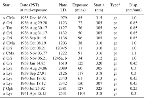
Table 1.Log of stellar spectrograms.
Star Date (PST) Plate Exposure Start λ Type* Disp.
at mid-exposure I.D. (mins) (nm) (nm/mm)
αCMa 1935 Dec 16.08 979 85 315 gr 1.0 βOri 1936 Aug 29.20 1123 22 305 pr 0.85 ζTau 1936 Aug 30.17 1127 76 305 pr 0.85 βOri 1936 Aug 31.17 1132 50 305 pr 0.85 γOri 1936 Sep 01.15 1136 96 305 pr 0.85 βCMa 1936 Oct 08.19 1203 38 310 gr 1.0 βOri 1936 Oct 08.21 1204/5 11 310 gr 1.0 ǫCMa 1936 Nov 03.77 1222 91 316 pr 1.1
βOri 1936 Nov 06.21 1245a, b 34 312 gr 1.0
βOri 1938 Jan 14.85 1610 125 320 gr 0.45 αLyr 1939 Aug 24.86 2089 60 305 gr 0.3 αLyr 1939 Sep 27.91 2126 117 318 gr 0.3 αLyr 1940 Jun 18.02 2340 61 313 gr 0.45 αLyr 1940 Jun 18.12 2342 150 307 gr 0.45 ζOph 1940 Jul 25.92 2381 127 325 gr 0.25 αLyr 1941 Apr 15.15 2531 110† 318 gr 0.3 * “pr” = prism spectrograph “gr” = grating spectrograph
† Note in log-book: “30% low cloud”
Fe-arc) exposed beside the stellar spectra for wavelength cal-ibration, and also scans of the plate background adjacent to the stellar exposure. Each scan was written as aFITS file, which was then interpreted with theIRAF2package.
3.2 Photometric calibration
A photographic emulsion has a non-linear response to light, so intensity calibration is essential for the extraction of re-liable line profiles. The calibration procedure, which has been well understood since the landmark paper by Hurter and Driffield (1890), requires an exposure of the same pho-tographic plate (or a piece of it) to laboratory sources of different but known intensities; in stellar spectroscopy it is common to employ a wedge or stepped entrance slit for the purpose. The relationship that is determined constitutes the emulsion’s “characteristic” or “H and D” (Hurter and Driffield) curve. In the UV and blue the slope of the curve changes only slowly with wavelength and the same curve may be considered reliable across a span of 20–30 nm or more.
Not all observers required (or saw fit to make) calibration exposures, and a few of the MW spectra did not include them. In such circumstances one might determine the curve from another spectrogram taken under similar conditions on the
2Image Reduction and Analysis Facility, developed and
main-tained by National Optical Astronomy Observatories (NOAO), Tuc-son, Arizona
same night, but without access to the log books it was not possible to discover where to locate such plates, since the archive is organized in order of positions of objects in the sky rather than plate number. In fact, because glass is opaque at the wavelengths of the Huggins bands the calibration expo-sures, which routinely used an ordinary light-bulb, faded to nothing below ∼350 nm. It was necessary, therefore, to se-lect a “reasonable” curve based on experience, assessing the goodness of the choice by comparing a resulting spectrum with one of the same (non-variable) object derived by other means.
The calibration techniques described by Griffin (1979) in-volved a purpose-built auxiliary spectrograph with quartz op-tics, and useful experience had been acquired with it con-cerning the nature of characteristic curves in the near UV for the relatively modern Eastman Kodak emulsions IIa-O and IIIa-J that were developed specifically for astronomy. Rela-tively late in this investigation a xerox copy (of a xerox copy) of the relevant Mount Wilson log-book was found, though of rather poor quality and missing column headers. The emul-sions that it named as in use before 1945 differed from mod-ern ones in that the emphasis was on high contrast rather than the detection of low light levels. High-contrast emulsions have much steeper curves than those of IIa-O (both IIa-O and IIIa-J were used to record the spectra analyzed in Paper 1), so the selection of calibration curves used here was adjusted appropriately.
The general characteristics of those historic emulsions could also have been investigated by deriving calibration curves at (say) 400 nm and comparing them to the curves for a better-researched emulsion such as IIa-O. Because the DAO’s PDS has latterly been out of commission that option could not be followed here, but will be considered seriously when handling historic spectra in the future.
3.3 Wavelength calibration
Stellar spectrograms usually include a laboratory (often an Fe-arc) spectrum as a wavelength reference adjacent to the stellar exposure. In the case of a prism spectrogram, calcu-lating a linear wavelength scale entails an interpolation based on the Hartmann formula (Hartmann 1898), and is satisfac-tory provided at least some reference lines are visible at all wavelengths. The extrapolations that were occasionally nec-essary in the present application were less reliable, but suf-ficiently good to enable the Huggins bands to be identified unambiguously.
In the case of grating spectra (the majority of the MW sam-ple) the derivation of a wavelength scale is intrinsically more precise. However, rather than relying on measured differ-ences between star lines and their arc counterparts and deriv-ing the radial-velocity shift (the classical method), it is more useful, when the radial velocity of the star is not required, to determine the wavelength scale by applying the grating equa-tion to a set of well-measured lines, as described by Griffin et al. (2000). By treating the arc lines first, one obtains the es-sential parameters (grating angle, order, camera focal length, etc.) and can then derive the wavelength scale of the stellar lines in their own rest-frame. The technique works faithfully to the observed limits of the stellar spectrum, and is applica-ble where there may not be any arc lines.
The stellar spectra, thus linearized in wavelength, were ex-tracted in steps of 0.001 nm or 0.005 nm, depending upon the nature, quality and dispersion of the original material (see Ta-ble 1). In two cases sequential exposures on the same object could be averaged, thus increasing the signal-to-noise ratio (S/N) of the final spectrum.
3.4 Observed stellar spectra
Each extracted stellar spectrum was normalized to the stellar continuum, a procedure which has been fully justified in Pa-per 1. It is important to point out that absolute stellar fluxes can not be determined from these ground-based observations, for the following reasons:
(a) The entrance slit of the spectrograph is narrower than the diameter of the stellar image so it restricts the fraction of the image that it admits, while atmospheric scintillation (“see-ing”) causes that fraction to vary significantly during an ex-posure and even over the course of a few seconds.
(b) The combination of telescope and spectrograph is less than fully efficient, and depends upon factors such as grating
and camera settings and optical reflectivity.
(c) Atmospheric refraction displaces and separates the violet image from the visible one, and can cause the former to miss the entrance slit altogether unless precautions are taken; the severity of the problem depends upon the position of the star in the sky and the quality of the seeing.
Through a combination of these factors the stellar flux recorded by the spectrograph is not a straightforward mea-sure of the light received by the telescope.
Particular care was taken to place the stellar continuum precisely at 100.0% at wavelength points outside the Hug-gins features. The latter are broad (∼1.5–2.5 nm) and shal-low (rarely dipping beshal-low ∼90% of the stellar continuum), so errors in continuum placement can be a dominant factor in the accuracy of the results.
In Fig. 1 the top four panels show stellar spectra that were extracted as described above. The laboratory “absorption” spectrum of O3in the lowest panel was derived from
Bass-Paur coefficients (Komhyr et al. 1993) by inverting the ab-sorption cross-sections, as detailed in Paper 1. Creation of the “cleaned” spectrum of α Lyr (Vega) in the third panel is described in Sect. 4.2.
Only about half of the borrowed sample of spectra even-tually proved useful for this project. Factors such as back-ground grain-noise and the detectability of faint broad fea-tures against a weak stellar exposure are assessed better from a density tracing than by eye. In a few spectra the S/N was generally too low to permit meaningful measurement of the O3 lines. In most of the other rejected cases the observed
wavelength span did not extend far enough into the UV to show more than a couple of Huggins features; those at the longest wavelengths are very weak and their measurements are correspondingly uncertain. Five plates of the bright early-A supergiant α Cyg (Deneb) were borrowed, but it was found that the stellar lines interfered even more seriously with the Huggins profiles than did those of η Ophiuchi (see Fig. 1, fourth panel). In one case a prism exposure (of an almost fea-tureless star spectrum) bore no wavelength reference spec-trum. The measurement of total O3 from the remaining 19
spectra exposed between 1935–1942 is described below.
4 Deriving O3columns
4.1 Basic Huggins-band measurements
In principle the fitting of a laboratory spectrum to the stel-lar features can be performed in a single step, the O3
col-umn being related to the factor required to achieve opti-mum fit. In practice, however, that route was not in the end followed (although experiments were made), because of the nature of the spectra being matched; the Huggins fea-tures are broad and shallow, and their profiles in a star can be adversely affected by variations in the local stellar con-tinuum level, whether caused by stellar blends or by
plate-R. E. M. Griffin: Measuring total ozone from historic stellar spectra 2235 ✂✁ ✒☎✄ ✚ ✞ í✡✠ ✐♠❫✷❛❜❭✌⑧❲❬➥♥⑨❭❘❬❂❦❧❴⑨❙❯❫♠q▼⑧➋❚♣❳❅❬❂❫❃❙❯❚❲➃❪❬❂❤✉❫✷❳✗❤✉❳❅❝✷❙➎❛✮❫✷⑧♣❚❲➃❪❬❂❤❣❫✷♥✺❤✗❬❂♥❵❦❧❙❯❚❲➄❘❬❂❤➦❚♣❳✉❴❵❢❅❬➥❴⑨❬❧➱♠❴❪q▼❭✌⑧❲❝✷❴⑨❴⑨❬❂❤❣❫❃♦✞❫✷❚➋❳✗♥⑨❴ ➢②❫❂✈✷❬❂⑧❲❬❂❳❅♦✷❴❵❢➆➼✲❚♣❳❀❳✗❛➛➚➎➘✣❬❂❫✷❦❯❢✽✈✷❬❪❙❵❴❵❚♣❦❪❫✷⑧❄♥❵❦❪❫✷⑧❲❬★❬❧➱✕❴⑨❬❂❳✦❤✗♥▼❞☛❙❵❝✞❛❒❽❪④✷④✠➳✕➌❃④❶➵✺❏❺❹➂❫❃❙❵❙❯❝✆➢❐♥⑨❴⑨❬❂⑧♣⑧♣❫❃❙➂❞❁❬❂❫❃❴❵➈❅❙❯❬❂♥➂❫❃❙❵❬★✈✕❚➋♥❵❚❲➄✦⑧❲❬ ❚♣❳★❴❵❢❅❬②❴⑨❝✷❭➫❭✦❫✷❳❅❬❂⑧✵➼✬ ❷✻❙❯❚↕q✷❫❺⑧♣❫❃❴⑨❬②➒❡➣➽❴✰✇☎❭❘❬➏♥❵➈✗❭✣❬❪❙❯♦✞❚♣❫✷❳❶❴➎➚➎q✷⑧❲❬❂♥❯♥❄♥❵❝✻❚♣❳★❴❵❢❅❬➧♥⑨❬❂❦❧❝✞❳✗❤➡❭✦❫✷❳✗❬❂⑧❘➼ ✮ ❷❺❙❯❚↕q✷❫✷❳➡❬❂❫❃❙❯⑧❲✇❸➒✩➣➽❴❇✇✕❭❘❬ ♦✞❚♣❫✷❳☎❴➎➚➎q❅➢▼❢✗❚♣⑧♣❬▼❚♣❳✮❴❵❢✗❬✻❞☛❝✞➈❅❙❵❴❵❢✺♥⑨❭❘❬❂❦❧❴⑨❙❯➈✗❛➩➼✝✆✤❷❺❭✦❢✵q☎❫➫❤❅➢②❫❃❙❵❞➐➉❺➔✕❏❖➌➫♥⑨❴❵❫❃❙✬➼✲❚♣❳✗❦❪⑧♣➈✦❤❅❬❂❤❨❢❅❬❪❙❯❬▼❞☛❝✷❙②❚➋⑧♣⑧♣➈✗♥⑨❴⑨❙➎❫❃❴❵❚❲❝✞❳❜❝✞❳✗⑧❲✇✗➚ ❴❵❢❅❬❪✇✯❚➋❳❶❴⑨❬❪❙❵❞☛❬❪❙❵❬✤♥⑨❬❪❙❯❚❲❝✞➈✦♥❵⑧❲✇✳➢▼❚❲❴❵❢✢❴❵❢❅❬✺❭✗❙❵❝✷➹✦⑧❲❬❂♥★❝✷❞➏❴❵❢❅❬➥❷❺➾❨❞❁❬❂❫❃❴❵➈✗❙❵❬❂♥❪❏ ⑩ ❢❅❬➛❴❵❢✗❚❲❙❯❤✢❭✦❫✷❳❅❬❂⑧✃♥❵❢❅❝✠➢▼♥➫❫ ✷⑨❦❪⑧❲❬❂❫✷❳✗❬❂❤☛✹ ♥⑨❭❘❬❂❦❧❴⑨❙❯➈✗❛ ❝✷❞↔➑↔❬❪♦✞❫P➼ ✫ ✰ ✇☎❙✆➘✌❴✰✇☎❭❘❬➫➉➂④❶➚➂❫❃❞☛❴⑨❬❪❙✻❴❵❢✗❬➡♥⑨❴⑨❬❂⑧➋⑧♣❫❃❙✻⑧➋❚♣❳❅❬❂♥▼❢✦❫❂✈✷❬➫➄❘❬❪❬❂❳❀❤✗❚♣✈✕❚♣❤✗❬❂❤✂❝✞➈❅❴❺➈✗♥❵❚♣❳❅♦➛❫➛♥⑨✇♠❳☎❴❵❢❅❬❪❴❵❚♣❦ ♥⑨❭❘❬❂❦❧❴⑨❙❯➈✗❛❮➼✲♥❵❬❪❬➫✐✕❬❂❦❧❴❪❏✗①❅❏❖➔✞➚➎❏ ⑩ ❢❅❬⑦➄❘❝✷❴⑨❴⑨❝✞❛ ❭✌❫✷❳❅❬❂⑧✵❚♣♥➧❫✮⑧♣❫❃➄❘❝✷❙❯❫❃❴⑨❝✷❙❯✇ ✷⑨❫❃➄✦♥❵❝✷❙❵❭✗❴❵❚❲❝✞❳☛✹❜♥❵❭✣❬❂❦❧❴⑨❙➎➈✗❛ ❝✷❞❡❷❺➾✛❏ ➅➇❳⑥➷➻❚❲♦❅❏➧❽✺❴❵❢❅❬✤❴⑨❝✷❭➆❞☛❝✞➈❅❙➫❭✦❫✷❳❅❬❂⑧♣♥➫♥❵❢❅❝✠➢ ♥⑨❴⑨❬❂⑧♣⑧♣❫❃❙❜♥⑨❭❘❬❂❦❧❴⑨❙❯❫✽❴❵❢✗❫❃❴➫➢✃❬❪❙❵❬✤❬❧➱✕❴⑨❙➎❫✷❦❧❴⑨❬❂❤➦❫✷♥✮❤❅❬❂♥❵❦❧❙➎❚❲➄❘❬❂❤✯❫❃➄❘❝✆✈✷❬✷❏ ⑩ ❢❅❬ ⑧♣❫❃➄❘❝✷❙❯❫❃❴⑨❝✷❙❵✇ ✷⑨❫❃➄✦♥⑨❝✷❙❵❭✦❴❵❚❲❝✞❳☛✹❺♥⑨❭❘❬❂❦❧❴⑨❙❯➈✗❛❐❝✷❞✵❷❺➾②❚♣❳➡❴❵❢❅❬➏⑧❲❝✆➢✃❬❂♥⑨❴↔❭✦❫✷❳✗❬❂⑧♠➢✃❫✷♥↔❤❅❬❪❙➎❚❲✈✷❬❂❤➫❞❁❙❯❝✞❛ ➒✃❫✷♥❯♥➇➣❇❾➻❫✷➈❅❙❡❦❧❝✕❬❪❱❨❦❪❚❲❬❂❳☎❴❵♥ ➼✲⑤⑦❝✞❛✮❢☎✇✕❙✻❬❪❴⑦❫✷⑧↕❏➻❽❂➓✷➓✷❻✞➚✻➄✕✇➥❚♣❳☎✈✷❬❪❙❵❴❵❚♣❳❅♦✺❴❵❢❅❬➫❫❃➄✦♥⑨❝✷❙❵❭✦❴❵❚❲❝✞❳❀❦❧❙❯❝✞♥❵♥➇➣❇♥⑨❬❂❦❧❴❵❚❲❝✞❳✦♥❪q➐❫✷♥⑦❤❅❬❪❴❵❫✷❚♣⑧❲❬❂❤✽❚♣❳✽❾➻❫❃❭✣❬❪❙❜❽❃❏★❿✃❙❯❬❂❫❃❴❵❚❲❝✞❳ ❝✷❞➻❴❵❢❅❬ ✷⑨❦❪⑧❲❬❂❫✷❳❅❬❂❤ ✹✮♥⑨❭❘❬❂❦❧❴⑨❙❯➈✗❛ ❝✷❞ ✫✱✰ ✇✕❙★➼☛➑↔❬❪♦✞❫❶➚➧❚➋❳✤❴❵❢❅❬✬❴❵❢✗❚❲❙➎❤✤❭✦❫✷❳❅❬❂⑧✵❚♣♥➧❤❅❬❂♥❯❦❧❙❯❚❲➄❘❬❂❤✂❚♣❳➥✐✕❬❂❦❧❴❪❏✗①❅❏❖➔✕❏ ❷❺❳✗⑧♣✇❸❫❃➄❘❝✞➈❅❴↔❢✗❫✷⑧❲❞✗❝✷❞✌❴❵❢❅❬➧➄❘❝✷❙❵❙❵❝✆➢✃❬❂❤➫♥❵❫✷❛❜❭✦⑧♣❬✃❝✷❞✣♥⑨❭❘❬❂❦❧❴⑨❙❯❫❺❬❪✈✷❬❂❳☎❴❵➈✗❫✷⑧♣⑧❲✇★❭✗❙❵❝✆✈✷❬❂❤❜➈✦♥⑨❬❪❞☛➈✦⑧☎❞☛❝✷❙↔❴❵❢✗❚♣♥❄❭✗❙❯❝✛➴➇❬❂❦❧❴❪❏↔➷✗❫✷❦❧❴⑨❝✷❙❯♥ ♥❵➈✗❦➎❢➊❫✷♥➏➄✌❫✷❦❵s✕♦✷❙❵❝✞➈✗❳✗❤✂♦✷❙➎❫✷❚♣❳♠➣❇❳❅❝✞❚♣♥❵❬❺❫✷❳✦❤✂❴❵❢❅❬✬❤❅❬❪❴⑨❬❂❦❧❴❵❫❃➄✦❚➋⑧♣❚❲❴❇✇✺❝✷❞➻❞☛❫✷❚➋❳❶❴➧➄✗❙❯❝✞❫✷❤✂❞❁❬❂❫❃❴❵➈✗❙❵❬❂♥➏❫❃♦✞❫✷❚♣❳✗♥❵❴▼❫❜➢✃❬❂❫❃s✤♥❵❴⑨❬❂⑧♣⑧♣❫❃❙ ❬❧➱♠❭✣❝✞♥❯➈❅❙❵❬➛❫❃❙❯❬✺❫✷♥❵♥❵❬❂♥❵♥⑨❬❂❤⑥➄❘❬❪❴⑨❴⑨❬❪❙➡❞☛❙❵❝✞❛❒❫❀❤✗❬❂❳✗♥❵❚❲❴✰✇❆❴⑨❙❯❫✷❦❪❚♣❳❅♦✽❴❵❢✗❫✷❳✢➄☎✇P❬❪✇✷❬✷❏✳➅➇❳✢❫❀❞☛❬❪➢ ♥⑨❭❘❬❂❦❧❴⑨❙❯❫❀❴❵❢❅❬➊✐ ✩✛❹Ï➢②❫✷♥ ♦✷❬❂❳❅❬❪❙❯❫✷⑧➋⑧❲✇✮❴⑨❝✕❝➫⑧♣❝✆➢➁❴⑨❝➫❭❘❬❪❙❯❛✮❚❲❴✃❛❜❬❂❫✷❳✗❚♣❳❅♦✷❞✲➈✗⑧✣❛❜❬❂❫✷♥❵➈❅❙❯❬❂❛❜❬❂❳❶❴②❝✷❞✚❴❵❢❅❬⑦❷ ➾ ⑧♣❚➋❳❅❬❂♥❪❏➻➅ç❳✺❛❜❝✞♥⑨❴➧❝✷❞✑❴❵❢❅❬❺❝✷❴❵❢❅❬❪❙➧❙❵❬ç➴⑨❬❂❦❧❴⑨❬❂❤ ❦❪❫✷♥⑨❬❂♥⑦❴❵❢✗❬➡❝✷➄✌♥⑨❬❪❙❵✈✷❬❂❤❆➢②❫❂✈✷❬❂⑧❲❬❂❳✗♦✷❴❵❢P♥⑨❭✦❫✷❳✳❤✗❚♣❤✳❳❅❝✷❴❺❬❧➱♠❴⑨❬❂❳✗❤✳❞✲❫❃❙⑦❬❂❳❅❝✞➈❅♦✞❢❆❚♣❳☎❴⑨❝✤❴❵❢❅❬❜t▼➑ ❴⑨❝✂♥❵❢❅❝✆➢Ö❛✮❝✷❙❵❬❜❴❵❢✗❫✷❳❆❫ ❦❧❝✞➈❅❭✦⑧♣❬➏❝✷❞✵➀➂➈❅♦✷♦✞❚➋❳✗♥↔❞☛❬❂❫❃❴❵➈❅❙❵❬❂♥❪➘♠❴❵❢❅❝✞♥⑨❬➂❫❃❴❡❴❵❢❅❬✻⑧❲❝✞❳❅♦✷❬❂♥⑨❴✶➢②❫❂✈✷❬❂⑧♣❬❂❳❅♦✷❴❵❢✗♥✃❫❃❙❵❬▼✈✷❬❪❙❵✇❜➢✃❬❂❫❃s✮❫✷❳✗❤❜❴❵❢✗❬❂❚❲❙✩❛❜❬❂❫✷♥❯➈❅❙❵❬❂❛❜❬❂❳☎❴❵♥ ❫❃❙❵❬❨❦❧❝✷❙❯❙❵❬❂♥⑨❭❘❝✞❳✗❤✗❚♣❳✗♦✞⑧❲✇➥➈✗❳✗❦❧❬❪❙❯❴❵❫✷❚♣❳✵❏✮➷➻❚❲✈✷❬✮❭✦⑧➋❫❃❴⑨❬❂♥⑦❝✷❞②❴❵❢❅❬✮➄✗❙❯❚♣♦✞❢❶❴❺❬❂❫❃❙❯⑧❲✇☎➣❇➉ ♥❵➈❅❭❘❬❪❙❵♦✞❚♣❫✷❳☎❴ ✫ ❿✃✇☎♦⑥➼✲❩➂❬❂❳✗❬❪➄✣➚✻➢✃❬❪❙❵❬ ➄❘❝✷❙❵❙❵❝✠➢✩❬❂❤✵q✵➄✌➈❅❴✻❚♣❴➂➢②❫✷♥⑦❞☛❝✞➈✗❳✗❤❀❴❵❢✗❫❃❴⑦❴❵❢❅❬❜♥⑨❴⑨❬❂⑧♣⑧♣❫❃❙⑦⑧♣❚➋❳❅❬❂♥➂❚➋❳❶❴⑨❬❪❙❵❞☛❬❪❙❵❬❂❤✽❬❪✈✷❬❂❳P❛❜❝✷❙❯❬➫♥❵❬❪❙❯❚❲❝✞➈✗♥❵⑧♣✇✂➢▼❚❲❴❵❢✽❴❵❢❅❬❜➀➂➈✗♦✷♦✞❚♣❳✗♥ ❭✗❙❵❝✷➹✌⑧❲❬❂♥▼❴❵❢✦❫✷❳✽❤✦❚♣❤➊❴❵❢❅❝✞♥❵❬➡❝✷❞✞✆✳❷✻❭✦❢✦❚♣➈✗❦❯❢✦❚❡➼✲♥⑨❬❪❬✮➷➻❚❲♦❅❏➻❽❃q✵❞❁❝✞➈❅❙❯❴❵❢➥❭✦❫✷❳✗❬❂⑧❁➚➎❏❺➅ç❳❀❝✞❳❅❬❜❦❪❫✷♥⑨❬❜❫✺❭✗❙❯❚♣♥❵❛ ❬❧➱✕❭❘❝✞♥❵➈✗❙❵❬✺➼☛❝✷❞ ❫✷❳➊❫✷⑧♣❛✮❝✞♥⑨❴②❞❁❬❂❫❃❴❵➈❅❙❯❬❂⑧❲❬❂♥❵♥➏♥⑨❴❵❫❃❙➂♥⑨❭❘❬❂❦❧❴⑨❙❯➈✗❛➛➚❡➄❘❝✷❙❵❬⑦❳❅❝❜➢②❫❂✈✷❬❂⑧❲❬❂❳❅♦✷❴❵❢➥❙❵❬❪❞☛❬❪❙❵❬❂❳✗❦❧❬✬♥⑨❭❘❬❂❦❧❴⑨❙❯➈✗❛➊❏ ⑩ ❢❅❬✬❛❜❬❂❫✷♥❵➈❅❙❯❬❂❛❜❬❂❳❶❴➧❝✷❞ ❴⑨❝✷❴❵❫✷⑧❄❷⑦➾❺❞❁❙❵❝✞❛ ❴❵❢❅❬⑦❙❵❬❂❛✮❫✷❚♣❳✦❚♣❳❅♦✂❽❂➓❜♥⑨❭❘❬❂❦❧❴⑨❙❯❫➫❬❧➱♠❭❘❝✞♥⑨❬❂❤✂➄❘❬❪❴❇➢✃❬❪❬❂❳✯❽❂➓✷❻✷➌✆➳✌❽❂➓✛①❶➔✤❚♣♥➧❤✗❬❂♥❵❦❧❙❯❚❲➄❘❬❂❤✺➄❘❬❂⑧❲❝✆➢✬❏ ❍➐✾★✂✁☎✙❃✟✠✟✑✟☛☞ ❀➆✫✮➾☛✡★✡✣✪☛✘❄✜⑥☞✑✖ ✂ ✄✝✆✞✄✌☞ ✜✕✔✩✙✑☞✎✍✑✏✻✸ ✸✣✙✝✼ ✔ ✺✹✼✌✜✣✼ ☎ ✑ ✡✗✜✕✔✒✏✰✏✌✡ ✑✢✡✭✼✚✍✝✔
Fig. 1. Sample spectra, linearized and normalized as described in the text, plotted against wavelength (in nm); each vertical scale extends from 100–50%. Narrow stellar features are visible in the top panel (β Ori, a late B-type supergiant), less so in the second panel (γ Ori, an early B-type giant), while in the fourth spectrum (η Oph, a dwarf A2.5 star (included here for illustration only) they interfere seriously with the profiles of the O3features. The third panel shows a “cleaned” spectrum of Vega (α Lyr; type A0) after the stellar lines have been divided out using a synthetic spectrum (see Sect. 4.2). The bottom panel is a laboratory “absorption” spectrum of O3.
background contamination. It therefore proved advantageous to deal with each O3 feature separately and to average the
final results.
A plot of the Huggins cross-sections reveals portions of “continuum” (corresponding to Hartley absorption only) be-tween the major Huggins features. The same portions were defined as “continuum” in the stellar spectra, thus defining the limits of the respective Huggins bands. The amount of absorption within each Huggins feature (its “equivalent width”, visualized as the width of a rectangular feature with the same total strength but a central absorption of 100%) was measured on-screen by interactive graphics. Where a star’s own absorption lines obviously contributed, the O3 profile
was sketched in with a smooth line. Each feature was mea-sured at least three times in order to ascertain the precision of the measurements. The spectrum of γ Ori, a hot B-type giant, shows almost no stellar features in 11 of the 12 visible O3features, so for that case (Ce 1136) a set of O3equivalent
widths was also measured by integrating the recorded inten-sities digitally, thus providing an indication of the accuracy of drawing a mean profile by hand.
4.2 “Cleaning” stellar spectra
As Paper 1 describes, a spectrum of Sirius observed from the ground can be “cleaned” of stellar features by dividing into it a spectrum of comparable resolution observed by the Hubble Space Telescope, i.e. above the Earth’s atmosphere. Unfor-tunately, owing to the wavelength restrictions of the space observation only 2 lines in the only MW spectrum of Sirius (Ce 979) could be thus “cleaned”; other features were mea-sured as described above. On the other hand, the six MW spectra of Vega could be fully “cleaned” by using the syn-thetic spectrum kindly provided by Dr. F. Castelli for use in Paper 1.
4.3 Conversion to O3columns
O3 columns (total O3) were derived as the ratio of stellar
to laboratory line strengths, as described in Paper 1. The measured stellar equivalent widths were plotted against the corresponding laboratory ones (“gf-values”); the latter were determined for Paper 1 by integrating the Bass-Paur O3
ab-sorption coefficients (Komhyr et al. 1993) and subtracting the smoothly-varying Hartley continuum. The relationship
passes through the origin by definition, and the gradient of each plot (giving the O3 column) was determined by
mini-mizing the distances of the points from it (“Least Absolute Residuals”). Two good examples of such a plot are given in Fig. 2; Fig. 2a was derived from measurements on a spec-trum of β Ori in the presence of stellar lines, while Fig. 2b corresponds to a “cleaned” spectrum of Vega. Because the ordinates are milli- ˚Angstr¨oms whereas the abscissae employ
˚
Angstr¨oms, the gradient is directly in Dobson Units (DU). In Paper 1 it was argued that Rayleigh and aerosol scat-tering are eliminated by the procedure adopted for extract-ing the O3information, and the same reasoning is accepted
here. Of the three types of atmospheric scattering or ab-sorption, only O3has a fine structure that can be discerned
as a wavelength-dependent variable. Other types of scatter-ing that vary only slowly with wavelength are eliminated by drawing the stellar continuum through points that correspond to maxima between the Huggins bands, so the O3
measure-ments are in effect made against a background of combined stellar and scattering continua. Even rapid changes in that smoothly-varying background will not affect the O3results
derived by this technique. 4.4 Air mass
The amount of atmospheric absorption encountered in a stel-lar observation depends upon the air mass, i.e. the path length through the atmosphere. Normalizing the observations to the same (zenithal) path length involves calculating the effective air mass from the mean angular elevation of the star in the sky; the air mass is close to sec z except at very large val-ues of z, the angular distance of the object from the zenith, though in stellar observing it may not be possible to make observations at zenith angles that substantially exceed ∼60◦.
Often the object’s hour angle (i.e. its angle from the merid-ian) is helpfully recorded by the observer at the beginning or end of an exposure, but if such information is not available it can be derived from the time of the observation plus the longitude of the observatory and the celestial coordinates of the star.
The air mass does not change appreciably during an ex-posure of about an hour or less, and a mean value can be adopted, though the altitude of the star is also critical. For Vega, which passes close to the zenith at Mount Wilson, the air mass increases by only 2% when the star is one hour away from its meridian passage, or 8% when two hours away, whereas for stars in Orion, which are some 50◦further south,
the minimum path length is about 60% greater than at the zenith and increases by 5% when one hour away from the meridian. With regard to the longer exposures recorded for some of the spectra in Table 1, four correspond to stars with southern declinations so the “effective” air mass is admit-tedly a rather coarse average.
The actual effective path length may differ from the mean if an exposure is interrupted by cloud, but unless the
log-book records such interruptions one has to assume that there were none. One of the observations used here did bear a comment regarding the state of the sky (see Table 1), though gave no guidance as to whether or how the exposure may have been prolonged. If an exposure is severely interrupted the response of the photographic plate to incident light may lose linearity (the well-known effect of “reciprocity failure”), in which case it would be necessary to model the exposure in terms of the percentage of full starlight received at different zenith distances. No information in that respect was offered – though most astronomers would not commence a lengthy exposure if it were likely to be interrupted by clouds. Un-weighted mean air masses were therefore adopted for all the spectra.
Table 2 lists the calculated air mass and the measured and normalized O3columns for each spectrum. The number of
lines used is a measure of the reliability of the derived O3
col-umn. The numbers in parentheses in col. 6 are the standard deviations associated with determining the best-fitting gradi-ent.
4.5 Errors affecting the results
The principal uncertainties in these results stem from: (1) Measuring errors. These are likely to be exacerbated when the S/N is low, or when there are enough stellar lines present to obscure a crucial part of the much broader O3
pro-file. Some idea of the magnitude of the measuring error was derived from repeated measurements on the same line, and (in the case of Ce 1136; Sect. 4.1) by comparing measure-ments made on hand-drawn profiles with the integrated in-tensities. In the latter exercise differences of a few percent were found, with a small bias that made the hand measure-ments mostly (but not always) lower, but in fact both the de-rived gradients and their formal fitting errors proved to be identical.
(2) Continuum placement. This is clearly critical in such broad features; a change in continuum level of only 0.5% alters the measurement of a line of characteristic shape (2– 2.5 nm wide and 10% deep) by about 5%, or 10% for a line only half as deep. Yet an error of 1% in levelling a rather noisy spectrum may be difficult to avoid.
(3) Photometric errors. These are harder to quantify, and may be anything up to ∼10% for a given plate. The fact that the procedure of dividing different spectra of Vega with the same low-noise synthetic spectrum produced only small mismatches in line-depth gave rise to cautious optimism. Pa-per 1 mentioned that small mismatches were also apparent in the “cleaned” spectra of Vega when the photometric cali-bration had been fully adequate, so part of those mismatches may in fact emanate from the synthetic spectrum. In general, if a calibration curve of incorrect slope is used the errors will be most prominent in the depths of strong lines, so one could conclude that the extent of those uncertainties here may be small, though probably not quite trivial.
R. E. M. Griffin: Measuring total ozone from historic stellar spectra 2237 ✂✁ ✒☎✄ ✚ ✞ ❀✜✠ ❩✻❬❪❴⑨❬❪❙❯❛✮❚➋❳✗❚♣❳❅♦✽❷⑦➾❨❦❧❝✞⑧♣➈✗❛❨❳✗♥❪q➏➼✲❫❶➚❸❞❁❙❵❝✞❛ ❭✦⑧♣❫❃❴⑨❬➊❿✃❬✳❽❂➔✛①❶➌❀❝✷❞ ✬ ❷✻❙❯❚❡❫✷❳✦❤➤➼☛➄❘➚⑦❞☛❙❵❝✞❛❒❫ ✷⑨❦❪⑧❲❬❂❫✷❳✗❬❂❤☛✹ ♥⑨❭❘❬❂❦❧❴⑨❙❯➈✗❛ ❝✷❞✶➑↔❬❪♦✞❫✤➄✦❫✷♥❵❬❂❤❀❝✞❳❀❭✦⑧♣❫❃❴⑨❬✮❿✃❬❜➔✷❻✛①✞④♠❏★◆➥❬❂❫✷♥❵➈❅❙❵❬❂❤✽❬❂➮✕➈✗❚❲✈❃❫✷⑧❲❬❂❳❶❴➂➢▼❚♣❤❅❴❵❢✦♥★➼✲❚♣❳✽➈✗❳✗❚❲❴❵♥➂❝✷❞▼❽❪④✁ ✂ ❳✗❛➛➚▼❫❃❙❵❬ ❭✦⑧❲❝✷❴⑨❴⑨❬❂❤✯❫❃♦✞❫✷❚♣❳✗♥⑨❴★❷❺➾★♦✷❞❁➣➽✈✛❫✷⑧♣➈✗❬❂♥❪❏ ⑩ ❢❅❬❜♦✷❙❯❫✷❤✗❚♣❬❂❳❶❴❺❝✷❞✃❴❵❢❅❬✮❤❅❝✷❴⑨❴⑨❬❂❤✯⑧➋❚♣❳❅❬➫❚♣♥❺❴❵❢❅❬➛❷❺➾➫❦❧❝✞⑧♣➈✗❛❨❳✽❚➋❳❆❩➂❝✷➄✌♥⑨❝✞❳Pt✻❳✗❚❲❴❵♥❪❏ ⑩ ❢❅❬⑦❬❪❙❯❙❵❝✷❙➏➄✦❫❃❙❯♥▼❫❃❙❵❬⑦❬❂♥⑨❴❵❚♣❛✮❫❃❴⑨❬❂❤❀➈✗❳✗❦❧❬❪❙❵❴❵❫✷❚➋❳❶❴❵❚❲❬❂♥▼❚♣❳✤❴❵❢❅❬✬❛❜❬❂❫✷♥❵➈✗❙❵❬❂❛❜❬❂❳☎❴❵♥★➼✲♥⑨❬❪❬➡✐♠❬❂❦❧❴❪❏✗①❅❏❖➌✞➚➎❏ ❫✛➭❘❬❂❦❧❴▼❴❵❢❅❬➡❷ ➾ ❙❯❬❂♥❵➈✗⑧❲❴❵♥➧❤❅❬❪❙➎❚❲✈✷❬❂❤✂➄✕✇➛❴❵❢✗❚➋♥②❴⑨❬❂❦❯❢✗❳✗❚➋➮☎➈❅❬✷❏ ✂ ✄✄✂ ✄✬✫ ✙✝✏ ✑ ✜✕✔✗✔ ⑩ ❢❅❬➡❫✷❛❜❝✞➈✗❳☎❴➂❝✷❞✩❫❃❴❵❛❜❝✞♥⑨❭✦❢❅❬❪❙➎❚♣❦✬❫❃➄✦♥⑨❝✷❙❯❭✗❴❵❚❲❝✞❳❀❬❂❳✗❦❧❝✞➈✗❳☎❴⑨❬❪❙❵❬❂❤✳❚♣❳➥❫✺♥⑨❴⑨❬❂⑧♣⑧♣❫❃❙➂❝✷➄✦♥⑨❬❪❙❵✈❃❫❃❴❵❚❲❝✞❳✳❤❅❬❪❭❘❬❂❳✗❤✗♥▼➈❅❭❘❝✞❳➊❴❵❢❅❬➫❫✷❚❲❙ ❛✮❫✷♥❵♥❂q▼❚↕❏➝❬✷❏❡❴❵❢✗❬❀❭✦❫❃❴❵❢❥⑧❲❬❂❳❅♦✷❴❵❢❣❴❵❢❅❙❵❝✞➈✗♦✞❢➦❴❵❢❅❬✳❫❃❴❵❛❜❝✞♥⑨❭✦❢✗❬❪❙❵❬✷❏✔❹➂❝✷❙❯❛✮❫✷⑧♣❚♣➃❂❚♣❳❅♦P❴❵❢❅❬✽❝✷➄✦♥⑨❬❪❙❯✈✛❫❃❴❵❚❲❝✞❳✦♥❨❴⑨❝⑥❴❵❢❅❬✳♥❵❫✷❛❜❬ ➼☛➃❪❬❂❳✗❚❲❴❵❢✦❫✷⑧❁➚✚❭✦❫❃❴❵❢✮⑧❲❬❂❳✗♦✷❴❵❢✮❚♣❳☎✈✷❝✞⑧❲✈✷❬❂♥❡❦❪❫✷⑧♣❦❪➈✦⑧♣❫❃❴❵❚♣❳❅♦❺❴❵❢❅❬➏❬❧➭❘❬❂❦❧❴❵❚❲✈✷❬✻❫✷❚❲❙❡❛✮❫✷♥❵♥✶❞❁❙❵❝✞❛Ö❴❵❢❅❬➏❛❜❬❂❫✷❳❨❫✷❳✗♦✞➈✗⑧♣❫❃❙↔❬❂⑧❲❬❪✈❃❫❃❴❵❚❲❝✞❳✮❝✷❞ ❴❵❢❅❬➧♥⑨❴❵❫❃❙❡❚➋❳❸❴❵❢❅❬➏♥❵s☎✇✣➘✞❴❵❢❅❬➧❫✷❚❲❙↔❛✮❫✷♥❵♥↔❚➋♥↔❦❪⑧❲❝✞♥⑨❬②❴⑨❝ ✔✖✡✗☞☎✄➻❬❧➱❅❦❧❬❪❭✗❴✶❫❃❴↔✈✷❬❪❙❵✇➡⑧♣❫❃❙❵♦✷❬②✈❃❫✷⑧♣➈❅❬❂♥➻❝✷❞☎✆✗q✞❴❵❢❅❬➧❫✷❳❅♦✞➈✗⑧♣❫❃❙↔❤✗❚➋♥⑨❴❵❫✷❳✗❦❧❬ ❝✷❞♠❴❵❢❅❬❡❝✷➄❅➴➇❬❂❦❧❴✚❞❁❙❵❝✞❛ ❴❵❢❅❬❡➃❪❬❂❳✦❚❲❴❵❢✵q✆❴❵❢✗❝✞➈❅♦✞❢❸❚♣❳❸♥⑨❴⑨❬❂⑧♣⑧♣❫❃❙✚❝✷➄✦♥⑨❬❪❙❵✈♠❚♣❳❅♦➏❚❲❴✚❛✮❫❂✇✬❳❅❝✷❴✑➄✣❬❡❭✣❝✞♥❯♥❵❚❲➄✦⑧❲❬➻❴⑨❝✻❛✮❫❃s✷❬❡❝✷➄✦♥❵❬❪❙❵✈✛❫❃❴❵❚♣❝✞❳✗♥ ❫❃❴➏➃❪❬❂❳✗❚♣❴❵❢✂❫✷❳❅♦✞⑧❲❬❂♥➧❴❵❢✗❫❃❴➏♥❯➈❅➄✦♥⑨❴❵❫✷❳☎❴❵❚♣❫✷⑧♣⑧❲✇❨❬❧➱♠❦❧❬❪❬❂❤✳➲⑦➬❃④✞✝➡❏✃❷✻❞☛❴⑨❬❂❳✂❴❵❢❅❬⑦❝✷➄♠➴⑨❬❂❦❧❴❪➸▲♥▼❢✗❝✞➈❅❙➏❫✷❳❅♦✞⑧❲❬❨➼✲❚↕❏➝❬✷❏✗❚♣❴❵♥➧❫✷❳❅♦✞⑧❲❬⑦❞☛❙❵❝✞❛ ❴❵❢❅❬✤❛❜❬❪❙❯❚♣❤✦❚♣❫✷❳✌➚✻❚♣♥★❢❅❬❂⑧❲❭✗❞✲➈✗⑧♣⑧❲✇❀❙❵❬❂❦❧❝✷❙❯❤❅❬❂❤✢➄✕✇P❴❵❢❅❬❨❝✷➄✌♥⑨❬❪❙❵✈✷❬❪❙❜❫❃❴★❴❵❢✗❬❨➄❘❬❪♦✞❚♣❳✗❳✗❚➋❳❅♦✂❝✷❙➫❬❂❳✗❤P❝✷❞▼❫✷❳✢❬❧➱♠❭✣❝✞♥❯➈❅❙❵❬✷q➻➄✦➈❅❴ ❚❲❞▼♥❯➈✗❦❯❢➆❚♣❳✗❞❁❝✷❙❯❛❨❫❃❴❵❚❲❝✞❳➨❚♣♥➫❳❅❝✷❴✮❫❂✈❃❫✷❚♣⑧♣❫❃➄✦⑧♣❬✺❚❲❴❜❦❪❫✷❳➆➄❘❬✂❤❅❬❪❙❯❚♣✈✷❬❂❤✢❞☛❙❵❝✞❛ ❴❵❢❅❬✤❴❵❚♣❛✮❬✺❝✷❞✻❴❵❢❅❬✤❝✷➄✦♥⑨❬❪❙❯✈✛❫❃❴❵❚❲❝✞❳➨❭✌⑧♣➈✗♥➡❴❵❢❅❬ ⑧❲❝✞❳❅♦✞❚♣❴❵➈✗❤❅❬❺❝✷❞➻❴❵❢❅❬⑦❝✷➄✦♥⑨❬❪❙❵✈❃❫❃❴⑨❝✷❙❵✇✂❫✷❳✗❤✂❴❵❢✗❬✬❦❧❬❂⑧❲❬❂♥⑨❴❵❚♣❫✷⑧➐❦❧❝✕❝✷❙❯❤✗❚➋❳✗❫❃❴⑨❬❂♥➧❝✷❞➻❴❵❢❅❬✬♥⑨❴❵❫❃❙❂❏ ⑩ ❢❅❬➂❫✷❚❲❙✩❛✮❫✷♥❯♥❡❤❅❝✕❬❂♥✩❳✗❝✷❴✩❦❯❢✦❫✷❳❅♦✷❬➂❫❃❭✗❭✦❙❵❬❂❦❪❚♣❫❃➄✦⑧❲✇➫❤✗➈❅❙➎❚♣❳❅♦✬❫✷❳✮❬❧➱♠❭❘❝✞♥❵➈❅❙❵❬▼❝✷❞➐❫❃➄✣❝✞➈✗❴❡❫✷❳➛❢✗❝✞➈❅❙✶❝✷❙②⑧❲❬❂♥❵♥❪q✕❫✷❳✗❤❨❫★❛❜❬❂❫✷❳ ✈❃❫✷⑧♣➈❅❬➧❦❪❫✷❳❜➄❘❬✃❫✷❤✗❝✷❭✗❴⑨❬❂❤✵q✞❴❵❢❅❝✞➈✗♦✞❢❜❴❵❢❅❬➧❫✷⑧❲❴❵❚❲❴❵➈✗❤✗❬✃❝✷❞✌❴❵❢❅❬➏♥⑨❴❵❫❃❙❡❚➋♥❄❫✷⑧➋♥⑨❝⑦❦❧❙❯❚❲❴❵❚♣❦❪❫✷⑧↕❏➻➷❅❝✷❙✶➑↔❬❪♦✞❫♠q✕➢▼❢✗❚➋❦❯❢➡❭✦❫✷♥❵♥⑨❬❂♥↔❦❪⑧♣❝✞♥⑨❬➧❴⑨❝ ❴❵❢❅❬➧➃❪❬❂❳✗❚♣❴❵❢✮❫❃❴✩◆➥❝✞➈✗❳❶❴❡➍❥❚♣⑧➋♥⑨❝✞❳✵q✷❴❵❢❅❬➏❫✷❚❲❙✩❛✮❫✷♥❵♥✶❚♣❳✦❦❧❙❵❬❂❫✷♥⑨❬❂♥↔➄✕✇★❝✞❳✦⑧❲✇➡➔✞➵✓➢➂❢❅❬❂❳❜❴❵❢❅❬➏♥⑨❴❵❫❃❙✩❚♣♥↔❝✞❳❅❬➏❢❅❝✞➈✗❙✶❫❂➢②❫❂✇❜❞☛❙❵❝✞❛ ❚❲❴❵♥➂❛❜❬❪❙❯❚♣❤✗❚➋❫✷❳➛❭✌❫✷♥❵♥❵❫❃♦✷❬✷q✣❝✷❙✻Ð✞➵ ➢➂❢❅❬❂❳✂❴❇➢✃❝✤❢❅❝✞➈❅❙❯♥➏❫✆➢✃❫✆✇✷q❘➢▼❢❅❬❪❙❵❬❂❫✷♥▼❞❁❝✷❙✻♥⑨❴❵❫❃❙❯♥▼❚➋❳❀❷✻❙❯❚❲❝✞❳➐q❅➢▼❢✗❚♣❦➎❢➊❫❃❙❵❬❸♥⑨❝✞❛✮❬➡➌❃④✞✝ ❞✲➈❅❙❵❴❵❢❅❬❪❙➏♥⑨❝✞➈✗❴❵❢✵q✗❴❵❢❅❬❸❛❨❚♣❳✗❚♣❛➡➈✗❛ ❭✦❫❃❴❵❢➊⑧❲❬❂❳✗♦✷❴❵❢➊❚♣♥➏❫❃➄❘❝✞➈❅❴➂➬❃④❶➵Ï♦✷❙❵❬❂❫❃❴⑨❬❪❙✻❴❵❢✗❫✷❳➊❫❃❴▼❴❵❢✗❬✬➃❪❬❂❳✗❚❲❴❵❢➊❫✷❳✦❤➊❚♣❳✗❦❧❙❵❬❂❫✷♥❵❬❂♥➧➄☎✇ ➌✞➵Ö➢▼❢❅❬❂❳❜❝✞❳❅❬✻❢❅❝✞➈❅❙❡❫✆➢✃❫✆✇✮❞☛❙❵❝✞❛Ö❴❵❢❅❬✻❛❜❬❪❙❯❚♣❤✦❚♣❫✷❳✵❏✑➍➤❚❲❴❵❢❨❙❵❬❪♦✞❫❃❙❯❤✮❴⑨❝★❴❵❢❅❬➂⑧♣❝✞❳❅♦✷❬❪❙❡❬❧➱♠❭❘❝✞♥❵➈❅❙❵❬❂♥↔❙❯❬❂❦❧❝✷❙❯❤❅❬❂❤✮❞☛❝✷❙②♥⑨❝✞❛❜❬ ❝✷❞❄❴❵❢❅❬⑦♥⑨❭❘❬❂❦❧❴⑨❙❯❫❜❚♣❳ ⑩ ❫❃➄✌⑧❲❬❜❽❃q❅❞❁❝✞➈❅❙➏❦❧❝✷❙❯❙❵❬❂♥⑨❭❘❝✞❳✗❤✺❴⑨❝✮♥⑨❴❵❫❃❙❯♥➧➢➂❚❲❴❵❢✤♥⑨❝✞➈❅❴❵❢❅❬❪❙❯❳✂❤✗❬❂❦❪⑧♣❚♣❳✗❫❃❴❵❚❲❝✞❳✦♥✩♥⑨❝❜❴❵❢✗❬ ✷➇❬❧➭✣❬❂❦❧❴❵❚❲✈✷❬✎✹➛❫✷❚❲❙ ❛✮❫✷♥❵♥▼❚♣♥➏❫✷❤✗❛✮❚♣❴⑨❴⑨❬❂❤✗⑧❲✇➛❫✮❙❯❫❃❴❵❢❅❬❪❙▼❦❧❝✞❫❃❙❯♥❵❬❸❫❂✈✷❬❪❙❯❫❃♦✷❬✷❏ ⑩ ❢❅❬➡❫✷❦❧❴❵➈✗❫✷⑧❄❬❧➭✣❬❂❦❧❴❵❚♣✈✷❬➡❭✌❫❃❴❵❢❀⑧❲❬❂❳✗♦✷❴❵❢➥❛✮❫✆✇➥❤✗❚➯➭❘❬❪❙▼❞☛❙❵❝✞❛ ❴❵❢❅❬➡❛✮❬❂❫✷❳❀❚❲❞↔❫✷❳✽❬❧➱♠❭✣❝✞♥❯➈❅❙❵❬❸❚♣♥✻❚♣❳☎❴⑨❬❪❙❵❙❯➈❅❭✦❴⑨❬❂❤✂➄☎✇❀❦❪⑧❲❝✞➈✗❤✵q ➄✦➈❅❴✃➈✗❳✗⑧❲❬❂♥❯♥✶❴❵❢❅❬⑦⑧❲❝✷♦❃➣➽➄❘❝✕❝✷s❜❙❵❬❂❦❧❝✷❙❯❤✗♥②♥❵➈✗❦➎❢✤❚♣❳❶❴⑨❬❪❙❯❙❯➈❅❭✗❴❵❚❲❝✞❳✦♥↔❝✞❳❅❬❺❢✗❫✷♥✃❴⑨❝➫❫✷♥❯♥❵➈✗❛❜❬➂❴❵❢✗❫❃❴②❴❵❢❅❬❪❙❵❬✻➢✩❬❪❙❵❬⑦❳❅❝✞❳✗❬✷❏✶❷⑦❳❅❬➂❝✷❞ ❴❵❢❅❬➂❝✷➄✦♥⑨❬❪❙❵✈❃❫❃❴❵❚❲❝✞❳✗♥✩➈✗♥⑨❬❂❤❨❢✗❬❪❙❵❬➂❤✗❚➋❤❜➄❘❬❂❫❃❙✩❫❸❦❧❝✞❛❨❛❜❬❂❳❶❴✃❙❵❬❪♦✞❫❃❙❯❤✦❚♣❳❅♦✬❴❵❢❅❬➂♥⑨❴❵❫❃❴⑨❬➂❝✷❞✵❴❵❢✗❬➂♥⑨s✕✇➥➼✲♥⑨❬❪❬ ⑩ ❫❃➄✦⑧❲❬➡❽✆➚➎q☎❴❵❢✗❝✞➈❅♦✞❢ ♦✞❫❂✈✷❬➊❳✗❝❀♦✞➈✗❚➋❤✗❫✷❳✗❦❧❬✤❫✷♥★❴⑨❝✳➢▼❢✗❬❪❴❵❢❅❬❪❙➫❝✷❙➫❢✗❝✆➢ ❴❵❢❅❬✺❬❧➱✕❭❘❝✞♥❵➈❅❙❯❬✺❛✮❫✆✇✯❢✗❫✆✈✷❬✂➄✣❬❪❬❂❳✢❭✗❙❵❝✞⑧♣❝✞❳❅♦✷❬❂❤✵❏✽➅✰❞▼❫✷❳⑥❬❧➱♠❭❘❝✞♥❵➈❅❙❵❬ ❚♣♥⑦♥⑨❬❪✈✷❬❪❙❯❬❂⑧❲✇❀❚♣❳☎❴⑨❬❪❙❵❙❯➈✗❭✗❴⑨❬❂❤✽❴❵❢❅❬❜❙❵❬❂♥⑨❭❘❝✞❳✗♥⑨❬➡❝✷❞✃❴❵❢❅❬❜❭✦❢❅❝✷❴⑨❝✷♦✷❙❯❫❃❭✌❢✗❚♣❦➡❭✦⑧♣❫❃❴⑨❬➫❴⑨❝➊❚♣❳✗❦❪❚➋❤❅❬❂❳❶❴❺⑧♣❚❲♦✞❢☎❴⑦❛✮❫❂✇✳⑧❲❝✞♥⑨❬❜⑧♣❚➋❳❅❬❂❫❃❙❯❚❲❴✰✇ ➼☛❴❵❢❅❬❜➢✃❬❂⑧♣⑧➯➣➽s♠❳❅❝✆➢➂❳❀❬❧➭❘❬❂❦❧❴✬❝✷❞ ✷➇❙❵❬❂❦❪❚❲❭✗❙❵❝♠❦❪❚❲❴✰✇➥❞✲❫✷❚♣⑧♣➈❅❙❵❬✎✹❶➚➎q✵❚♣❳✽➢▼❢✦❚♣❦❯❢✳❦❪❫✷♥⑨❬❨❚♣❴➂➢✃❝✞➈✗⑧♣❤✽➄❘❬❜❳❅❬❂❦❧❬❂♥❵♥❵❫❃❙❵✇✽❴⑨❝➊❛❜❝♠❤❅❬❂⑧❄❴❵❢❅❬ ❬❧➱♠❭✣❝✞♥❯➈❅❙❵❬❀❚➋❳➦❴⑨❬❪❙❯❛✮♥➛❝✷❞⑦❴❵❢❅❬✽❭❘❬❪❙❯❦❧❬❂❳❶❴❵❫❃♦✷❬✳❝✷❞⑦❞✲➈✗⑧♣⑧➏♥❵❴❵❫❃❙❯⑧♣❚❲♦✞❢☎❴❨❙❵❬❂❦❧❬❂❚♣✈✷❬❂❤❥❫❃❴✤❤✗❚➯➭❘❬❪❙❵❬❂❳☎❴❨➃❪❬❂❳✗❚♣❴❵❢✉❤✗❚♣♥❵❴❵❫✷❳✗❦❧❬❂♥❪❏ ❹➂❝ ❚♣❳❅❞☛❝✷❙❯❛✮❫❃❴❵❚♣❝✞❳❨❚♣❳➛❴❵❢✗❫❃❴②❙❵❬❂♥⑨❭❘❬❂❦❧❴✃➢✃❫✷♥②❝❃➭❘❬❪❙❵❬❂❤❨➳✮❴❵❢❅❝✞➈❅♦✞❢✤❛❜❝✞♥⑨❴②❫✷♥⑨❴⑨❙❵❝✞❳❅❝✞❛✮❬❪❙❯♥②➢✩❝✞➈✦⑧♣❤➛❳✗❝✷❴✃❦❧❝✞❛✮❛✮❬❂❳✗❦❧❬⑦❫➡⑧♣❬❂❳❅♦✷❴❵❢❶✇ ❬❧➱♠❭✣❝✞♥❯➈❅❙❵❬✬❚❲❞➻❚❲❴➧➢✃❬❪❙❵❬★⑧♣❚♣s✷❬❂⑧❲✇❨❴⑨❝➛➄✣❬✬❚➋❳❶❴⑨❬❪❙❵❙➎➈❅❭✗❴⑨❬❂❤✤➄✕✇✤❦❪⑧♣❝✞➈✗❤✗♥❪❏❡t✻❳☎➢✩❬❂❚❲♦✞❢☎❴⑨❬❂❤✽❛❜❬❂❫✷❳➥❫✷❚❲❙➂❛✮❫✷♥❵♥⑨❬❂♥▼➢✩❬❪❙❵❬❸❴❵❢❅❬❪❙❵❬❪❞☛❝✷❙❵❬ ❫✷❤❅❝✷❭✗❴⑨❬❂❤➊❞❁❝✷❙✻❫✷⑧♣⑧❘❴❵❢❅❬✬♥⑨❭❘❬❂❦❧❴⑨❙❯❫♠❏
Fig. 2. Determining O3columns, (a) from plate Ce 1245 of β Ori and (b) from a “cleaned” spectrum of Vega based on plate Ce 2340. Measured equivalent widths (in units of 10−4nm) are plotted against O
3gf-values. The gradient of the dotted line is the O3column in
Dobson Units. The error bars are estimated uncertainties in the measurements (see Sect. 4.5).
Table 2.Determinations of Zenithal O3.
Star Date (PST) Plate Air No. of Raw O3 Zenithal Arosa O3 at mid-exposure I.D. Mass Lines (DU) O3(DU) (DU)
1 2 3 4 5 6 7 8 αCMa 1935 Dec 16.08 979 1.63 9 478 (7) 294 320 (19) βOri 1936 Aug 29.20 1123 1.46 13 409 (9) 280 297 (20) ζTau 1936 Aug 30.17 1127 1.30 12 350 (9) 269 296 (19) βOri 1936 Aug 31.17 1132 1.63 12 375 (9) 230 293 (14) γOri 1936 Sep 01.15 1136 1.52 12 359 (8) 236 293 (14) βCMa 1936 Oct 08.19 1203 1.58 10 547 (10) 346 321 (15) βOri 1936 Oct 08.21 1204/5 1.44 11 441 (6) 306 321 (15) ǫCMa 1936 Nov 5.77 1222 2.19 8 718 (15) 329 292 (30)
βOri 1936 Nov 06.21 1245a,b 2.00 11 638 (8) 319 292 (19)
βOri 1938 Jan 14.85 1610 1.44 5 537 (25) 373 315 (22) αLyr 1939 Aug 24.86 2089 1.01 12 332 (5) 329 303 (11) αLyr 1939 Sep 27.91 2126 1.47 6 535 (12) 364 291 (12) αLyr 1940 Jun 18.02 2340 1.01 9 421 (7) 417 366 (11) αLyr 1940 Jun 18.12 2342 1.16 11 499 (13) 430 366 (11) ζOph 1940 Jul 25.92 2381 1.74 3 566 (36) 325 324 (16) αLyr 1941 Apr 15.15 2531 1.05 5 411 (26) 391 383 (38)
(4) Laboratory gf-values. As there are no other measure-ments against which to compare the values used here, it is not possible to derive realistic error estimates. This matter was examined in some depth in Paper 1, where a consistency test was devised to investigate the likelihood and magnitude of such errors. Since the laboratory spectra were low-noise one has reasonable confidence that the measurements of the laboratory line strengths contain much smaller uncertainties than the measurements made on stellar spectra. For each measured O3feature an uncertainty was computed by adding
quadratically an error of 100 (in units of 10−4nm), based
upon an assumed continuum error of 0.5% and scaled accord-ing to the actual width of the line, to the range in measured equivalent widths indicated by repeated measurements on the
same feature. Those uncertainties are depicted as vertical er-ror bars in Figs. 2a and 2b. No contribution in respect of possible photometric errors has been included, as their mag-nitude is as yet unknown. It should also be noted that no con-tributions from SO2have been included in this work; such an
investigation would only be meaningful when a much larger database of O3columns has been derived and any errors in
the individual measured strengths of the laboratory features can first be more completely understood.
5 Comparison with solar data
Two significant sources of solar data are available: Arosa (Switzerland) and Table Mountain (California). The Arosa
✂✁ ✒☎✄ ✚✞ ❁ ✠ ❷❺➾❺❦❧❝✞⑧♣➈✦❛✮❳✗♥❪q❅❚♣❳✂❩❺t★q✗❤❅❬❪❙❯❚❲✈✷❬❂❤✤❞☛❙❵❝✞❛ ◆➥➍ ♥⑨❭❘❬❂❦❧❴⑨❙❯❫➫✈✷❬❪❙❯♥❵➈✗♥✬➼✲❳✕➈✗❛❜❬❪❙➎❚♣❦❪❫✷⑧❁➚✩❦❪❫✷⑧❲❬❂❳✗❤✗❫❃❙➂❛❜❝✞❳❶❴❵❢➐❏ ⑩ ❢❅❬ ❬❪❙❵❙❵❝✷❙▼➄✦❫❃❙❯♥➏❚♣❳✦❤✗❚♣❦❪❫❃❴⑨❬❺❞❁❝✷❙➎❛✮❫✷⑧➐➈✗❳✗❦❧❬❪❙❯❴❵❫✷❚♣❳❶❴❵❚♣❬❂♥✬➼✲♥⑨❬❪❬ ⑩ ❫❃➄✦⑧❲❬❸➔✞➚➎❏ ✂✁✒☎✄ ✚✞ ❄ ✠ ❷❺➾✯❦❧❝✞⑧♣➈✗❛✮❳✗♥❀❤❅❬❪❙❯❚❲✈✷❬❂❤ ❞❁❙❯❝✞❛ ◆➥➍ ♥⑨❭❘❬❂❦❧❴⑨❙❯❫✓➼✲❤❅❝✷❴❵♥➎➚➥❦❧❝✞❛❜❭✦❫❃❙❵❬❂❤✔❴⑨❝❣✈❃❫✷⑧♣➈❅❬❂♥➥❞❁❙❯❝✞❛ ❴❵❢❅❬⑥➉▼❙❯❝✞♥❵❫ ❤✗❫❃❴❵❫❃➄✦❫✷♥❵❬✷❏✩➷❅❝✷❙➂❴❵❢❅❬✬♥❵❫❃s✷❬❸❝✷❞➻❦❪⑧♣❫❃❙❯❚♣❴❇✇✷q✗❴❵❢❅❬❸❬❪❙❵❙❵❝✷❙➏➄✦❫❃❙➎♥✬➼☛♦✞❚❲✈✷❬❂❳➥❚♣❳ ⑩ ❫❃➄✦⑧❲❬❸➔✞➚➧❢✗❫❂✈✷❬➡❳❅❝✷❴➧➄❘❬❪❬❂❳➊❚♣❳✗❦❪⑧♣➈✦❤❅❬❂❤✵❏ í✞❀
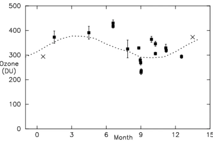
Fig. 3. O3columns, in DU, derived from MW spectra versus (nu-merical) calendar month. The error bars indicate formal uncertain-ties (see Table 2).
database contains measurements for ∼200 days per year dur-ing the period in question, but the Table Mountain data are much more sparse and contain only ∼20–40 values per year. There are also differences in the nature of the measurements, as discussed below. However, in view of the close proxim-ity of Mount Wilson and Table Mountain it was important to include a comparison.
5.1 Arosa Dobson data
Mount Wilson and Arosa are both mid-latitude northern-hemisphere sites but separated in longitude by 128◦.
Nev-ertheless, it was useful to make a comparison between the results derived in this paper with the values recorded for the same dates in the extensive database of daily Arosa measure-ments (available from WOUDC). However, while there ap-pears to be a globally linked pattern in O3columns there are
also substantial local variations caused by meteorological in-fluences. In order to avoid undue emphasis on local varia-tions a mean was taken of the five Arosa values nearest to the date of the stellar observation; the day-to-day variations over the same period were also averaged. It is those means and their average daily excursions that are included in the final column of Table 2.
In Fig. 3 the O3 results from Mount Wilson are plotted
against calendar month, and clearly demonstrate the seasonal variation. The dotted line shows the run of Arosa monthly means. Apart from a group of observations in late August (all in fact from the same period in 1936) there is a tendency for the stellar results to be 5–10% higher than the Arosa ones. It was pointed out in Sect. 4.3 that these stellar results are independent of Rayleigh and aerosol scattering. However, inasmuch as they give total O3they include tropospheric as
well as stratospheric ozone. Mount Wilson Observatory, at an altitude of 1742 m, is only 100 m lower than the Arosa sta-tion, though it is located close to what is now a region of
sig-nificant anthropogenic air-quality compromise. That some daytime pollution has long affected the site was admitted in Abbot’s efforts to monitor the solar constant from a num-ber of world sites, including Mount Wilson, between 1900– 1950 (e.g. Abbot, Fowle and Aldrich 1923). Daily observa-tions at MW, commencing in 1905, were routinely halted at 10 a.m. when the general atmospheric transparency (includ-ing an increase in water vapour) began to deteriorate, but the use of the site for work of such sensitivity apparently drew some criticism, and in 1920 the project at MW was discon-tinued. However, a night-time inversion layer prevents the pollution in the valley from mixing with the purer air at the level of the Observatory, and since not all the stellar values are higher than the Arosa ones it seems unlikely that large amounts of tropospheric O3were included in the stellar
mea-surements.
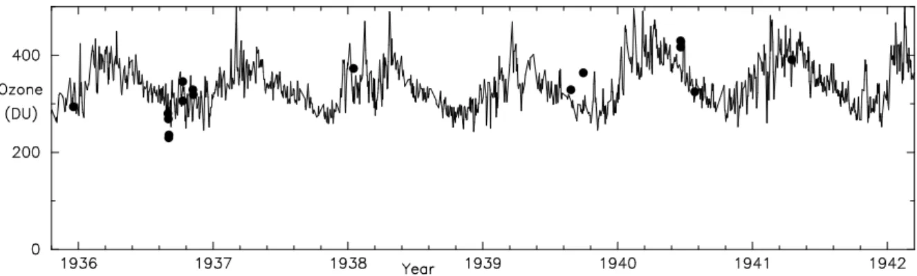
In Fig. 4 the stellar results are compared again a time-sequence of daily Arosa measurements. In that plot the ten-dency for the stellar values to be higher than the solar-derived ones is more disguised as occasionally (e.g. in January 1938) the stellar value corresponds to a brief peak in the Arosa data. It is also noticeable in that figure that the four low stellar re-sults were closely grouped 1936. From such a small sample it is not possible to separate technical problems from pat-terns of real, local variability. The four spectra in question were all exposed in the 9-ft focal-length quartz-prism spec-trograph, on different emulsions but ones that were not exclu-sively used then, and involving stars that gave higher results on later dates. The only exclusive commonality is the spec-trograph; however, an overplot of Ce 1204+5 and 1245 (both are spectra of β Ori, but the latter was observed 3 months later than the “low-O3” period and with a different camera
and grating set-up) show very close agreement between the strengths of the stellar features. Although more conclusive evidence, e.g. from other observations made during that pe-riod, and/or from other spectra with the same equipment out-side that period, cannot be provided at this stage, what is to hand indicates that the low values of O3 during mid-1936
were probably real, at least qualitatively.
The difference in latitude of some 12 degrees between the two sites may introduce additional uncertainty in this com-parison. TOMS data for Los Angeles are regularly about 25 DU lower than for Arosa, with considerably larger occasional excursions (Peter 2006, private communication), though the same systematic difference may not bave pertained 40–50 years earlier when the stellar spectra examined here were ob-served; for example, the distribution and percentage of tro-pospheric O3at Mount Wilson may have changed. Again, a
much larger stellar sample is needed in order to distinguish between systematic and random differences.
It may be significant that the Mount Wilson O3 columns
determined for late 1939 and 1940 are somewhat high, as are also the Arosa values at that time (see Fig. 4); the smoothed running mean of Arosa data exhibits an appreciable peak. In a recent investigation of this curiosity Br¨onnimann et
R. E. M. Griffin: Measuring total ozone from historic stellar spectra 2239 ❷❺➾❺❦❧❝✞⑧♣➈✦❛✮❳✗♥❪q❅❚♣❳✂❩❺t★q✗❤❅❬❪❙❯❚❲✈✷❬❂❤✤❞☛❙❵❝✞❛ ◆➥➍ ♥⑨❭❘❬❂❦❧❴⑨❙❯❫➫✈✷❬❪❙❯♥❵➈✗♥✬➼✲❳✕➈✗❛❜❬❪❙➎❚♣❦❪❫✷⑧❁➚✩❦❪❫✷⑧❲❬❂❳✗❤✗❫❃❙➂❛❜❝✞❳❶❴❵❢➐❏ ⑩ ❢❅❬ ❬❪❙❵❙❵❝✷❙▼➄✦❫❃❙❯♥➏❚♣❳✦❤✗❚♣❦❪❫❃❴⑨❬❺❞❁❝✷❙➎❛✮❫✷⑧➐➈✗❳✗❦❧❬❪❙❯❴❵❫✷❚♣❳❶❴❵❚♣❬❂♥✬➼✲♥⑨❬❪❬ ⑩ ❫❃➄✦⑧❲❬❸➔✞➚➎❏ ✂✁✒☎✄ ✚ ✞ ❄ ✠ ❷❺➾✯❦❧❝✞⑧♣➈✗❛✮❳✗♥❀❤❅❬❪❙❯❚❲✈✷❬❂❤ ❞❁❙❯❝✞❛ ◆➥➍ ♥⑨❭❘❬❂❦❧❴⑨❙❯❫✓➼✲❤❅❝✷❴❵♥➎➚➥❦❧❝✞❛❜❭✦❫❃❙❵❬❂❤✔❴⑨❝❣✈❃❫✷⑧♣➈❅❬❂♥➥❞❁❙❯❝✞❛ ❴❵❢❅❬⑥➉▼❙❯❝✞♥❵❫ ❤✗❫❃❴❵❫❃➄✦❫✷♥❵❬✷❏✩➷❅❝✷❙➂❴❵❢❅❬✬♥❵❫❃s✷❬❸❝✷❞➻❦❪⑧♣❫❃❙❯❚♣❴❇✇✷q✗❴❵❢❅❬❸❬❪❙❵❙❵❝✷❙➏➄✦❫❃❙➎♥✬➼☛♦✞❚❲✈✷❬❂❳➥❚♣❳ ⑩ ❫❃➄✦⑧❲❬❸➔✞➚➧❢✗❫❂✈✷❬➡❳❅❝✷❴➧➄❘❬❪❬❂❳➊❚♣❳✗❦❪⑧♣➈✦❤❅❬❂❤✵❏ í✞❀
Fig. 4. O3columns derived from MW spectra (dots) compared to values from the Arosa database. For the sake of clarity, the error bars (given in Table 2) have not been included.
al. (2004) demonstrated a correlation between an increase in the Arosa O3 columns (and in others recorded during that
period) and a particularly intense and long-lasting El Ni˜no episode. If the correlation has a physical explanation it would be interesting to investigate it from a much larger database of Mount Wilson stellar measurements.
5.2 Table mountain measurements
A long-term project set up by C. G. Abbot, Director of the Smithsonian Astrophysical Observatory (SAO), Wash-ington, to investigate the constancy of the sun’s output pro-duced low-resolution bolometric tracings of the solar spec-trum throughout the visible region from a number of (mostly high-elevation) stations worldwide. Produced variously be-tween 1902 and 1961, the spectral scans show absorption from atmospheric constituents such as CO2, water-vapour
and the Chappuis bands of O3, and have been studied to
determine changes in atmospheric transparency due to sus-pended aerosols, to examine correlations between water-vapour and local vegetation, and to measure total O3 –
e.g. Angione, Medeiros and Roosen (1976), Roosen and An-gione (1977, 1984). One of the SAO stations was on Table Mountain (TM), California, only about 50 km from Mount Wilson. Total O3was measured there between 1925–1948.
Another station was also set up on Mount Wilson itself, but was discontinued after a relatively short span, as already mentioned.
The Chappuis bands are rather weak features in the re-gion ∼530–650 nm. The analysis by Anre-gione, Medeiros and Roosen (1976) found a correlation coefficient of 0.7 between O3results between TM and Arosa values, though a modern
study by Br¨onnimann finds that the TM values are system-atically lowered by at least 6% (Br¨onnimann, 2005, private communication). The fact that different bands are used may be significant; the Huggins bands are temperature-sensitive whereas the Chappuis bands are not, but the latter are much more badly affected by aerosol scattering, and are
intrinsi-cally weaker and are therefore also more prone to scattered light contamination. According to Br¨onnimann (loc. cit) the scale of the TM results also depends upon which of the Chap-puis bands is measured: the one at 615 nm yields consider-ably smaller values than does the one at 574 nm. Fig. 5 com-pares the stellar values with the TM ones, after an increase of 10% has been applied to the latter. Despite the scale prob-lems, such a comparison is useful for studying relative vari-ations, i.e. for illustrating precision rather than accuracy, at this point, particularly since the uncertainties attributable to a latitude difference, as mentioned in the previous Section, do not apply.
The overall conclusion of this paper is that historic O3columns can be recovered from archived stellar spectra
with sufficient precision that the patterns which they depict will be of significant value to studies of the natural behaviour and evolution of the ozone layer.
Since the astronomical observations are not in digital form, the extraction of information in units that are meaning-ful for atmospheric science is inevitably a somewhat involved process. While some streamlining of the methods outlined above is possible for handling larger volumes of data, there is no shortcut to the amount of personal attention that needs to be applied at all stages of the transformation from photo-graph to scientific measurement. The hope, for the future, is that all of astronomy’s relevant historic (i.e. photographic) observations shall be digitized, forming a database that will offer free access for all purposes, not only for the search for signatures of O3.
Acknowledgements. This work has been supported by the Cana-dian Foundation for Climate and Atmospheric Sciences through Grant GR-338, Measuring Ozone Columns from Astronomical Archives. I am indebted to colleagues at York University and Environment Canada, naming in particular J. McConnell and D. Wardle, for their patience and persistence in trying to teach me the rudiments of atmospheric science while grappling with the apparent inconsistencies of stellar spectroscopy, and I am very grateful to the Dominion Astrophysical Observatory for continuing