Ørsted Initial Field Model

HAL Id: insu-01410544

https://hal-insu.archives-ouvertes.fr/insu-01410544

Submitted on 6 Dec 2016

HAL is a multi-disciplinary open access

archive for the deposit and dissemination of

sci-entific research documents, whether they are

pub-lished or not. The documents may come from

teaching and research institutions in France or

abroad, or from public or private research centers.

L’archive ouverte pluridisciplinaire HAL, est

destinée au dépôt et à la diffusion de documents

scientifiques de niveau recherche, publiés ou non,

émanant des établissements d’enseignement et de

recherche français ou étrangers, des laboratoires

publics ou privés.

Ørsted Initial Field Model

N Olsen, R Holme, G Hulot, T Sabaka, T Neubert, C Toffner-Clausen, P

Primdahl, J Jorgensen, J. Léger, D Barraclough, et al.

To cite this version:

N Olsen, R Holme, G Hulot, T Sabaka, T Neubert, et al.. Ørsted Initial Field Model. Geophysical

Re-search Letters, American Geophysical Union, 2000, 27 (22), pp.3607-3610. �10.1029/2000GL011930�.

�insu-01410544�

Orsted

Initial

Field Model

N. Olsen

•, R. Holme

2, G. Hulot 3, T. Sabaka

4, T. Neubert

s,

L. TOffner-Clausen

•, F. Primdahl

•,6, J. Jorgensen

6, J.-M. L6ger

7,

D. Barraclough

8, J. Bloxham

ø, J. Cain

•ø, C. Constable

TM,

V. Golovkov

•2

A. Jackson

•3 P. Kotz• TM B Langlais

3 S Macmillan

8 M. Mandea

3

J. Merayo

•, L. Newitt • M Purucker

4 T Risbo

• M. Stampe

•

A. Thomson

s, C. Voorhies

4

Abstract. Magnetic measurements taken by the Orsted

satellite during geomagnetic quiet conditions around Jan- uary 1, 2000 have been used to derive a spherical harmonic model of the Earth's magnetic field for epoch 2000.0. The maximum degree and order of the model is 19 for internal, and 2 for external, source fields; however, coefficients above degree 14 may not be robust. Such a detailed model exists for only one previous epoch, 1980. Achieved rms misfit is < 2 nT for the scalar intensity and < 3 nT for one of the vector components perpendicular to the magnetic field. For scientific purposes related to the Orsted mission, this model supercedes IGRF 2000.

Introduction

Twenty years after the Magsat mission, the Orsted satel- lite was launched on February 23, 1999 in a near polar orbit with an inclination of 96.5 ø, a perigee at 638 km and an apogee at 849 km. The principal aim of the Orsted mission is to map accurately the Earth's magnetic field.

The goal of this paper is to present an accurate "snap- shot" of the geomagnetic field at epoch 2000.0 based on geomagnetic quiet days around January 1, 2000. To reduce contamination of the lower degree expansion coefficients by spatial aliasing, the analysis was performed through degree

and order 19 for the internal field and 2 for the external

field. However, we only recommend use of coefficients up to degree 14 at most.

Orsted data from May to September 1999 were used to

derive the IGRF 2000 [Olsen et al., 2000]. However, the

Danish Space Research Institute, Copenhagen, Denmark

2GeoForschungsZentrum, Potsdam, Germany

alPGP, Paris, France

4NASA/GSFC, Greenbelt/MD, USA

5Danish Meteorological Institute, Copenhagen, Denmark

6Institute for Automation, DTU, Lyngby, Denmark

7CEA-Direction des Technologies Avanc•es, France

SBritish Geological Survey, Edinburgh, UK

9Harvard University, Cambridge MA, USA

løFlorida State University, Tallahassee, FL, USA

•University of California, San Diego, CA, USA

•2IZMIRAN, Troitsk, Russia •aUniversity of Leeds, UK

14Hermanus Magnetic Observatory, S. Africa

•SNatural Resources Canada

•6Copenhagen University, Denmark

Copyright 2000 by the American Geophysical Union.

Paper number 2000GL011930. 0094-8276/00/2000GL011930505.00

satellite was still in the commissioning phase before Septem- ber 1999, and the measurements used for the present study

are more accurate.

Data selection and pre-processing

Data from geomagnetic quiet conditions between Decem- ber 18, 1999 and January 21, 2000 were selected according to the following criteria: Kp <_ 1-t- for the time of observation,

Kp <_ 20 for the previous three hour interval, IDstl < 10 nT

and d(Dst)/dt I < 3 nT/hr. To reduce contributions

from

ionospheric currents at middle and low latitudes, only night-

side data (local time about 22:00) were selected. Vector

data were used for dipole colatitudes 40 ø < 0dip • 140 ø (0dip defined by the first three coefficients of IGRF 2000), and scalar data for 190- Odip l • 500 or if attitude data were

not available. To further reduce contributions from polar

cap ionospheric currents, only data for which B•, the dawn- dusk component of the interplanetary magnetic field (IMF,

in GSM coordinates)

was weak (IB•l < 3 nT) were used.

An equal area distribution was approximated by decimat-

ing the data to measurement times at least 30s/sin 0 apart,

where 0 is geocentric co-latitude. All orbits were visually inspected and those suspected of contamination by exter-

nal currents were removed. Attitude information over the

South Atlantic Anomaly (SAA) was sparse

due to radiation

effects on the star imager, resulting in a paucity of vector data there. Since this region is close to the dip-equator

(the thin line in Figure 1) where vector data are mandatory

to avoid the Backus effect [Stern and Bredekamp, 1975], 66

data points during four orbits on the geomagnetic quiet days October 9 and November 26, 1999 were added to constrain field direction in this region. Figure I shows the distribution of the 2148 scalar data points and 3957 vector triplets used for the model.

The attitude accuracy of the Orsted star imager (SIM) is

anisotropic: determination of the SIM bore-sight direction

("pointing") is more accurate than determination of the ro- tation around the bore-sight ("rotation"). This results in

relatively more noise in the rotation angle, which is also more sensitive to distorting effects like instrument blinding

(for instance by the moon). This attitude anisotropy results

in correlated errors between the orthogonal magnetic com- ponents traditionally used for modeling, which should be

taken into account when deriving field models [Holme and Bloxham, 1996; Holme, 2000].

Let • be the unit vector of the SIM bore-sight, and let

B be the observed magnetic field vector. B and • define a new coordinate system (provided they are not parallel),

and the magnetic

residual

vector 5B - (SBs, 5Bñ, 5Ba) can

3608 N. OLSEN ET AL.:ORSTED INITIAL FIELD MODEL Table 1. Number Ntot of data points, number Nout of removed

outliers, means, and rms misfits (in nT) for the different compo-

nents retained. "Polar" denotes data with [90- 0dip[ ) 50 ø. (•Fpolar 5Fnon-polar '-]- 5BB 5Ba 5B,• 5Bo

I N tot

1322

4783

3957

3957

be transformed such that the first component, 5BB, is in the direction of B, the second component, 5Bx, is aligned

with (•xB), and the third component,

5Ba, is aligned

with

B x (•xB). The last two components

are perpendicular

to

the magnetic field. In this coordinate system, the errors on the different field components are uncorrelated.

Let •b be the attitude error of the bore-sight (pointing error), X that around bore-sight (rotation error) and let cr be the (attitude independent) error of the scalar intensity.

Considering only linear terms in •b and X, the component 5Bs is independent of attitude errors. 5Ba is affected only by pointing errors, whereas 5Bx is influenced by both point-

ing errors and rotation errors [Holme, 2000]. Since the ro-

tation uncertainty is believed to be the main error source, the component Bx is more contaminated than the two other components and should be down-weighted.

As an example, Figure 2 shows the residuals of the nightside part of orbit # 4343. The upper panels present

residuals

(SB,•,SBo,SB4) as a function of colatitude 0; the

lower panels present the residuals

as (SBs, 5Bx,SBa). The

noise is clearly spread over all three components in the

(SB,.,SBo,SB4) system, but is concentrated in 5Bñ in the (SBs,SBx,SBa) system. 5Ba is slightly noisier than 5Bs

due to pointing uncertainty and field-aligned currents. In particular, 5Ba signatures at 0 • 25 ø and 170 ø are caused by auroral field-aligned currents. The gap in the vector com- ponents between 0 = 100 ø and 135 ø is due to moon-blinding of the star imager.

Most data selected span 35 days during which the field

changes

by up to 20 nT due to secular variation (SV). It

has been decided to account for this change by propagat- ing all observations to epoch 2000.0 using a model of the

SV since this a) reduces the model misfit of 5BB and 5Ba

180' 240' 300' O' 60' 120' 180'

Figure 1. Data distribution. Scalar measurements are shown by

small and vector measurements by larger symbols. Open circles present additional vector data to fill the gap in the SAA.

Table 2. Expansion coefficients of internal (g•m, h•m) and exter-

nal (q•m,s•m) contributions, in nT. q•m and g•m present the Dst-

dependent part of the external coefficients.

n m g• 0 1 0 1 2 1 1 2 2 2 3 3 3 3 4 4 4 4 4 5 5 5 5 5 5 6 6 6 6 6 6 6 7 7 7 7 7 7 7 7 8 8 8 8 8 8 8 8 8 9 9 9 9 9 9 9 9 9 9 10 10 10 10 -29617.37 -1729.24 -2268.46 3068.92 1670.76 1340.16 -2288.34 1252.09 714.08 932.11 786.66 249.82 -403.30 111.25 -217.06 351.98 222.06 -130.52 -168.40 -12.92 71.40 67.40 74.17 -160.81 -5.77 17.00 -90.38 79.07 -73.59 -0.04 33.10 9.11 7.03 7.o8 -1.31 23.92 5.99 -9.20 -7.74 -16.54 8.95 7.03 -7.97 -7.01 5.30 9.63 2.93 -8.58 6.32 -8.76 -1.53 9.13 -4.24 -8.09 -3.03 -6.46 1.56 -2.95 m 5185.65 -2481.77 -457.62 -227.87 293.28 -491.32 273.21 -231.70 119.53 -303.65 42.76 171.19 -132.88 -39.42 106.44 -16.86 64.34 65.34 -61.03 0.80 43.96 -65.03 -24.69 6.17 24.03 14.87 -25.34 -5.71 12.18 -21.05 8.63 -21.39 15.30 8.76 -14.92 -2.46 -19.91 13.07 12.50 -6.23 -8.31 8.46 3.88 -8.29 4.88 1.87 0.34 4.12 m 0.36 1.29 -0.85 -2.59 0.90 -0.65 -2.82 -0.89 -1.08 -1.98 -0.44 -0.40 0.25 2.38 -2.66 0.54 0.29 0.02 -0.03 0.21 -1.00 -0.48 0.54 -0.81 0.23 1.79 -0.49 -0.95 -0.03 0.63 0.21 0.62 0.29 -0.23 -0.24 -1.03 0.12 -O.74 0.19 0.40 -0.11 0.42 0.20 0.26 0.30 0.03 -0.03 0.05 0.04 0.21 m -3.73

Table 2 continued m n m g2 h2 n m q2 sn 10 4 -0.32 4.94 2 0 1.57 10 5 3.67 -5.86 2 I 0.29 -0.32 10 6 1.11 -1.18 2 2 -0.52 -0.04 10 7 2.09 -2.84 10 8 4.41 0.24 n m • • 8n 10 9 0.42 -1.98 I 0 -0.59 10 10 -0.94 -7.67 i I 0.04 0.10

by 10% and 6%, respectively

(that of 5B j_ is not changed);

and b) reduces the magnetic power Rn for all degrees above

n = 12 (mean reduction per degree: 17%). The latter indi-

an updated version of the IGRF 2000 SV model [Macmillan and Quinn, 2000] and a model generated from Orsted data spanning 9 months. Negligible difference was found, so it was decided to use the Orsted SV model for internal consis- tency. This model is still in development, and will be the subject of a future publication.

0 30 90 120 150 180 , ! i , 2O 'o ' 0 30 60 9 120 150 180

-20

2ø

t

'

,

? or---'

...

-20

]-

• ø

/ ••

Figure 2. Residuals (observations minus values predicted by the

model of Table 2) as a function of co-latitude 0 for the nightside

part of orbit • 4343, December 22, 1999, 01:21 - 02:11 UT. Kp =

0o and Dst = +9 nT. o lO lO o lO lO ß i i i ß . . ß ß .._. ß : ." : .f•... : .." . •: r •- .•.• ... ,: .•g,; •.. ,., :.... ;.. o

•B

3

•;,•

• ,...,

,•.'•.:•,

...•....,

,.: • • ',

....

:

...

; ...

:.'.'..::::.:

... ; ... :

....

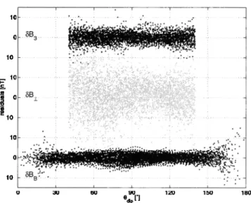
Figure 3. Residuals as a function of dipole co-latitude.

Model parameterization

and estimation

The magnetic field B -- -grad V can be derived from a magnetic scalar potential V which is expanded in terms of spherical harmonics:

V a

=

(g•

cos

m4

+ h: sin

m4) a n+Z

-

P; (cos

,•

O)

n--1 •r•-- 0

•

r PF (cos

O)

+ .

(q•cosm•+

s• sinm•) •

n=l •=0

[qV(coO) +

;l

V?(coO)]

a = 6371.2 km is the mean radius of the Earth, (r, 0,•)

are geocentric coordinates, P• (cos0) are the associated

Schmidt-normalized

Legendre

functions and (g•,h•)

and

(q•, s•) are the Gauss coefficients describing internal and

external source

fields, respectively.

The coefficients

•, •

and • account

for the Dst-dependent

part of the external

dipole. Its internal, induced, counterpart is represented via

the factor Q:: 0.27, a value found from Magsat data by

[Langel and Estes, 1985] (The results are rather insensitive to the exact value of Qz since only data for which JDstJ • 10 are used). The model has 410 parameters (399 static inter-

nal, 8 static external, and 3 coefficients

of Dst-dependency).

The coefficients are estimated by an iterative least-squares

fit, minimizing

eTC•Ze where

the residuals

e: dobs--

d•nod

are the differences between observations and values pre- dicted by the model, and Ca is the a priori covariance of

residuals due to data errors and fields left unmodeled. To

account for the anisotropic attitude accuracy, Ca was as-

signed the form of Eq. 18 of Holme and Bloxham [1996],

with cy: 2.25 nT, • = 10" and X = 60" (these values

are

justified by the a posteriori model misfit; pre-fiight instru-

ment error estimates were 3", 3" and 20" for SIM angles

and 0.2 nT for the vector magnetometer

magnitude).

When solving the least-squares problem, three iterations were found to be sufficient for convergence. Outliers were removed after the second iteration; as outlier selection cri-

31510 N. OLSEN ET AL.:ORSTED INITIAL FIELD MODEL

5Bñ. If one of the component residuals was above its thresh- old value, all three components were removed. All but one

of the 49 vector outliers are due to ]SBñ] • 30 nT and are

probably associated with single "spikes" in the attitude data

(cf. 5Bñ of Figure 2).

Results and Discussion

Number of data points fitted, residual means and rms misfits of the model are given in Table 1. The anisotropy

of rms misfit in (SBB, 5Bñ, 5B3) components is much larger

than in spherical components. Figure 3 shows the data resid- uals as a function of dipole co-latitude. The largest residuals

in 5BB are found in the southern polar cap (•}dip

• 170

ø)

and are attributed to ionospheric currents in the summer polar cap. Electrical conductivity is smaller in the north-

ern (winter) polar cap ionosphere due to absence of solar

irradiation, and therefore the 5Bs residuals in the northern

polar cap (•}dip • 10 ø) exhibit a smaller scatter than their

counterparts in the southern polar cap. However, contribu- tions from ionospheric polar electrojets are present even in

the northern auroral zone (•}dip

• 23ø).

The large rms value for 5Bñ (present even when the data are weighted isotropically) confirms the necessity to down-

weight this component using the covariance matrix Ca. A

resolution analysis [Tarantola, 1987] shows that Bñ resolves

only 6% of the model parameters if the data are treated in this way, but 24% if data errors are assumed to be isotropic.

The corresponding

values for BB (B3) are 38% (27%) and

27% (23%), whereas the resolving

power of F is 30% and

27%, respectively. The model fits the data with a (normal- ized) chi-squared misfit of 1.01, consistent with the weight- ing (a priori data errors or, •h, X) being correct. Note also the non-zero mean value for 5Bñ (though much smaller than the rms value). We currently have no explanation for this

non-zero mean.

The model coefficients are given in Table 2. Only inter-

nal coefficients up to n: 14 are listed (Coefficients above

n - 14 are not considered robust because they typically change by over 20% under plausible increases in the trunca-

tion level from 19 to 23); the complete model is available at

www.

dsri.dk

/ Oersted/Field_models

/ O IFM/.

Experiments with various truncation levels of the spheri- cal harmonic expansion gave the largest changes close to the southern magnetic pole. This indicates that contributions from ionospheric current systems in the summer hemisphere are probably present in the data and model in spite of our attempt to minimize external current contributions by care-

ful data selection according to geomagnetic indices and IMF

By.

To address these contributions will likely require inclu- sion of more satellite data, ground data, and perhaps co- estimation of ionospheric field parameters, which is beyond the scope of our model.

This initial model from Orsted, the first magnetic map-

ping mission of the "International Decade of Geopotential Research", provides a firm basis for studies of the iono- spheric, magnetospheric, lithospheric and core fields. It will also aid interpretation of the additional, continuous, high precision measurements of Earth's time-varying geo- magnetic and gravitational fields acquired by forthcoming missions like Champ and SAC-C.

Acknowledgments. The Orsted Project was made pos-

sible by extensive support from the Ministry of Trade and Indus- try, the Ministry of Research and Information Technology and the Ministry of Transport in Denmark. Additional international and crucial support was provided from NASA, ESA, CNES and DARA.

References

Holme, R., Modelling of attitude error in vector magnetic data: application to Orsted data, Earth, Planets and Space, in press,

2000.

Holme, R., and J. Bloxham, The treatment of attitude errors in satellite geomagnetic data, Phys. Earth Planet. Int., 98, 221-

233, 1996.

Langel, R. A., and R. H. Estes, The near-Earth magnetic field at 1980 determined from MAGSAT data, J. Geophys. Res., 90,

2495-2509, 1985.

Macmillan, S., and J. M. Quinn, The 2000 revision of the joint

UK/US geomagnetic field models and an IGRF candidate

model, Earth, Planets and Space, in press, 2000.

Olsen, N., T. J. Sabaka, and L. Toffner-Clausen, Determination of the IGRF 2000 model, Earth, Planets and Space, in press,

2000.

Stern, D. P., and J. H. Bredekamp, Error enhancement in geo- magnetic models derived from scalar data, J. Geophys. Res., 80, 1776-1782, 1975.

Tarantola, A., Inverse Problem Theory - Methods for Data Fit- ting and Model Parameter Estimation, Elsevier, New York,

1987.

N. Olsen, Danish Space Research Institute, Jullane Maples Vej

30, DK- 2100 Copenhagen O, Denmark. (e-mail: [email protected])

(Received June 21, 2000; revised August 1, 2000; accepted September 1, 2000.)