HAL Id: insu-03192554
https://hal-insu.archives-ouvertes.fr/insu-03192554
Submitted on 8 Apr 2021
HAL is a multi-disciplinary open access
archive for the deposit and dissemination of
sci-entific research documents, whether they are
pub-lished or not. The documents may come from
teaching and research institutions in France or
abroad, or from public or private research centers.
L’archive ouverte pluridisciplinaire HAL, est
destinée au dépôt et à la diffusion de documents
scientifiques de niveau recherche, publiés ou non,
émanant des établissements d’enseignement et de
recherche français ou étrangers, des laboratoires
publics ou privés.
Distributed under a Creative Commons Attribution| 4.0 International License
Multi-phase seismic source imprint of tropical cyclones
Lise Retailleau, Lucia Gualtieri
To cite this version:
Lise Retailleau, Lucia Gualtieri. Multi-phase seismic source imprint of tropical cyclones. Nature
Com-munications, Nature Publishing Group, 2021, 12 (1), �10.1038/s41467-021-22231-y�. �insu-03192554�
Multi-phase seismic source imprint of tropical
cyclones
Lise Retailleau
1,2✉& Lucia Gualtieri
3✉
The coupling between the ocean activity driven by winds and the solid Earth generates seismic signals recorded by seismometers worldwide. The 2–10 s period band, known as secondary microseism, represents the largest background seismic wavefield. While moving over the ocean, tropical cyclones generate particularly strong and localized sources of sec-ondary microseisms that are detected remotely by seismic arrays. We assess and compare the seismic sources of P, SV, and SH waves associated with typhoon Ioke (2006) during its extra-tropical transition. To understand their generation mechanisms, we compare the observed multi-phase sources with theoretical sources computed with a numerical ocean wave model, and we assess the influence of the ocean resonance (or ocean site effect) and coastal reflection of ocean waves. We show how the location and lateral extent of the associated seismic source is period- and phase-dependent. This information is crucial for the use of body waves for ambient noise imaging and gives insights about the sea state, complementary to satellite data.
https://doi.org/10.1038/s41467-021-22231-y OPEN
1Université de Paris, Institut de physique du globe de Paris, CNRS, Paris, France.2Observatoire Volcanologique du Piton de la Fournaise, Institut de physique
du globe de Paris, La Plaine des Cafres, France.3Department of Geophysics, Stanford University, Stanford, CA, USA. ✉email:[email protected];
123456789
O
cean storms generate seismic signals through coupling between ocean waves and the solid Earth1–3. The sec-ondary microseism—the strongest background seismic energy of the Earth—is generated by the nonlinear interaction between pairs of sets of ocean gravity waves with overlapping frequency content and opposite directions. The period of the resulting seismic waves—between 2 and 10 s—is half the period of the involved ocean waves. Extreme events, such as tropical cyclones, are among the most efficient storms to generate sec-ondary microseisms4, whose sources are well-localized. Tropicalcyclones rotate counterclockwise in the northern hemisphere while moving over the ocean. As theorized by Longuet-Higgins5,
when they overrun their previously generated waves, ocean wave–wave interactions occur in the tail of the events themselves. The seismic sources of ocean storms were observed first by analyzing body-wave signals at seismic arrays6–9. Stacking the
arrivals of a seismic phase recorded at an array of stations allows for increasing its signal-to-noise ratio and linking the seismic phase to its source10. Specific events have been identified and studied
through the lens of seismology, such as hurricane Katrina11,
typhoon Ioke12, hurricane Sandy13, and hurricane Bill14. A vast majority of these studies focused on the extraction of the most energetic signals, at narrow period bands, and over a limited period of time. Retailleau and Gualtieri15 extended these analyses and were able to seismically track the path of typhoon Ioke (2006) throughout its entire life cycle and over the whole period band of secondary microseisms. All these studies focused on retrieving the sources of compressional P waves. Using the classical beamforming analysis technique, very few studies have extracted the signal associated with shear S waves16–19, as they have low amplitude,
often below the noise level20. As a consequence, there is a big gap of knowledge on the location and generation mechanisms of sec-ondary microseism S waves.
The cross-correlation of the ambient seismic wavefield data (often referred to as “ambient noise”) has been shown to be complementary to earthquake data for imaging the Earth’s structure through surface seismic waves21. More recently, the cross-correlation technique has been used successfully to extract body waves and information about the deep structure of the Earth22–24. This technique relies on the hypothesis that the
sources of ambient noise are equipartitioned. The nonuniform distribution of sources and the lacking comprehension of the signal are the main limitations for imaging the Earth through ambient-noise body waves25. Indeed, errors and uncertainties
associated with source location and mechanisms affect cross-correlation measurements26and do not allow for discriminating
between source- or structure-originating velocity variations27. In
particular, S waves, which are the commonly used seismic phases for deep Earth imaging28, are challenging to retrieve, with
sig-nificant uncertainties associated with them. As a consequence, the retrieval of body-wave phases for deep Earth imaging so far has focused mostly on P waves. Knowledge of the sources is crucial, both in terms of location and lateral extent, to image the sub-surface reliably.
In this study, we focus on extracting the complete body-wave (compressional and shear) imprint of typhoon Ioke (Fig. 1a). Typhoon Ioke was one of the longer-lasting tropical cyclones in the Pacific Ocean and the most intense ever recorded in the Central Pacific. It occurred in August–September 2006, and it is one of the few tropical cyclones to reach Category-5 status on the Saffir–Simpson Scale in the Central and North Pacific Ocean. We do not only focus on locating the maximum seismic energy imprint, but also on evaluating the lateral extent of the sources. We use the Southern California seismic data29 (Fig. 1a, b) to identify and locate the seismic sources of typhoon Ioke using the back-projection method10developed by Retailleau et al.30,31. This
method was adapted to study P-wave sources of typhoon Ioke by Retailleau and Gualtieri15.
Results
Inferring the seismic sources. While Retailleau and Gualtieri15
focused on retrieving the track of the event by locating P-wave sources, here we focus on the latest part of the event, during which the typhoon made the tropical–extratropical transition (around 30∘N), from September 2 to 6 2006, before becoming an extratropical storm. In particular, we extract the body-wave phases generated by the typhoon from seismograms recorded by 129 stations in Southern California29. We perform
back-projection10 analysis in the rotated radial–transverse-coordinate
b)
Seismic stations Ioke Satellite data
Seismic sources P SH SV a) c) Selected days
Fig. 1 Typhoon Ioke, seismic stations, and associated body-wave sources. a Satellite track of typhoon Ioke (cyan) and Southern California stations (brown).b Zoom over the Southern California seismic stations used in this study for locating the sources of typhoon Ioke. c Locations of body-wave seismic sources in the 4–6 s period band (P-wave sources are in red, SV-wave sources in blue, and SH-wave sources is green). The two circled arrows in panelsa and c mark the two locations of the typhoon studied in this paper.
system to extract the P, SV, and SH seismic phases and enhance the quality of the signals. Further details regarding satellite and seismic data can be found in Supplementary Note 1. Further details about the data analysis technique are in “Methods”. As verified by Retailleau et al.30,31, this method is able to correctly
locate earthquake sources worldwide. To further assess the array response and estimate the influence of the Earth’s 3D structure and topography on our measurements, we perform classical beamforming analyses10 on synthetic signals obtained by
employing the SPECFEM3D_GLOBE package32,33. We use a
single source at the location of the typhoon and three different Earth models, and compare the beamforming results of P, SV, and SH waves (for more details, see Supplementary Note 2). Our analysis of synthetic data reveals that the presence of topography does not have a significant effect on the retrieval of sources of P, SV, and SH waves. The retrieval of P-wave sources is not influ-enced either by 3D heterogeneities (Supplementary Fig. 1). The influence of the 3D Earth’s structure on the retrieval of SV (Supplementary Fig. 2) and SH (Supplementary Fig. 3) waves is more difficult to assess as they are poorly generated in the absence of heterogeneities, coherently with recent findings on Love waves34. Further studies will be needed to quantify the effect of
3D heterogeneities on the generation and propagation of S waves. Figure1c shows the location of the maximum seismic energy associated with P, SV, and SH waves during the typhoon tropical-extratropical transition in the period band 4–6 s. As observed by Retailleau and Gualtieri15, P-wave sources (red dots) follow the typhoon track (cyan) during the entire life cycle of the event, confirming the generation theory proposed by Longuet-Higgins in 19535. Shear-wave sources (blue and green dots) are more
scattered and tend to follow the track only along portions of it or their amplitude is too small to be observed. Indeed, SV-wave sources are located close to the event before the tropical–extratropical transition, while they get scattered after-ward. SH-wave sources are located close to the typhoon track only between 30∘and 40∘N, while they are scattered at lower and higher latitudes. Among these three body-wave phases, P waves are confirmed to be the best proxy for typhoon track.
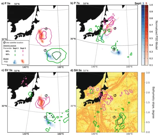
Ambient-noise sources generated by storms in the ocean are not earthquake-like point sources. In order to study the lateral extent of the source and better understanding the source mechanisms, we focus our analysis on two periods of time (circled arrows in Fig. 1a, c), before and after the tropical–extratropical transition. During these two periods of time, Ioke’s dynamic was very different and the event was located in two very different environments. On September 3 at 18:00 UTC, the typhoon was a Category 2 event on the Saffir–Simpson scale with a maximum sustained wind speed of 48.87 m/s. It was located far away from the coast in a deep-water environment. Contrarily, on September 5 at 18:00 UTC, the typhoon was weaker and classified as a tropical storm with a maximum sustained wind of 28.29 m/s. At that time, Ioke approached the Japanese coast, though still in a deep-water environment.
Comparing observations with models. Recent developments in modeling the seismic sources of secondary microseisms from ocean-wave action models35–37 allowed to make predictions of
the location of the seismic sources of P- and SV waves20and to
simulate the amplitude of P waves38. However, important ques-tions are still open, such as the effect of the reflection of ocean waves at the coast and the effect of the bathymetric roughnesses on the source location and lateral extent.
In afirst effort to compare both location and lateral extent of observed and simulated body-wave sources, we compute synthetic P- and SV-wave sources using the ocean-wave model
WAVEWATCH III37. The model returns the pressure power
spectral density (PSD) due to the ocean wave–wave interaction which can occur offshore, far away from continents, or close to the coast, due to the reflection of ocean waves. Coastal reflection is not well-constrained as it depends on many factors, such as the shape of the coast. The model allows for excluding coastal reflection or for including it, up to a maximum coastal reflection coefficient of 10%37. Like in Retailleau et al.31, we use this value to
include sources due to coastal reflection (see Supplementary Note 3, for a comparison of the sources with and without coastal reflection). Moreover, we correct the pressure PSD for the ocean site effect20, which accounts for the reverberation of P waves in
the water column (see“Methods” and Supplementary Note 3). At 5-s period (Fig.2a), the seismic energy of P waves (contour lines) is located in the tail of the typhoon both on September 3 and 5 (green and pink contour lines, respectively). The modeled P-wave sources at 5-s period (blue and red shadows for September 3 and 5, respectively) predict well the observed sources. However, synthetic sources appear to be confined closely behind the event, especially on September 3, while the observed seismic energy covers a larger area away from the typhoon. Both observed and synthetic sources show energy along the track of the typhoon, in the open ocean, and no clear effect of the coast is observed. The observed source is very well resolved (see the results of the bootstrap analysis in Supplementary Note 4, Supplementary Fig. 5a).
At 7-s period, the observed and synthetic energy associated with P waves are not only located in the tail of the typhoon but also along the coast of Japan (Fig. 2b). Both observed and synthetic sources show a coastal component either on September 3, when the event is still in the open ocean and on September 5, when it approaches the coasts of Japan. To understand what caused the sources close to the coasts of Japan, we compute synthetic sources with and without coastal reflection and ocean site effect (Supplementary Note 3 and Supplementary Fig. 4). Because ocean waves are dispersive by nature, the long-period waves are expected to move ahead and reach the coast before the short-period waves. However, we verified that the contribution of the dispersion of ocean gravity waves to the pressure PSD associated with the nonlinear ocean wave–wave interaction is several orders of magnitude smaller than the sources in the open ocean (Supplementary Fig. 4a). Both coastal reflection and ocean site effect contribute to the emergence of these sources. While the coastal reflection is likely the dominant generation mechanism for these sources (Supplementary Fig. 4c), the ocean site effect (Supplementary Fig. 4b) contributes to reshaping the lateral extent of the source (Supplementary Fig. 4d). It is the ocean site effect that allows the synthetic sources to assume a northwest–southeast shape, similarly to the observed sources. We note, however, that the observed seismic sources are, on average, closer to the Japanese coast than synthetic sources, potentially due to the uncertainties in constraining the ocean-wave reflection coefficient in our modeling.
Shear-wave analysis. Shear-wave sources remain largely unex-plained so far, because of the low amplitude and signal-to-noise ratio of these seismic phases. We extract shear-wave energy at 5 s for the two selected periods of time (Fig. 2c, d). Observed and synthetic sources associated with SV waves show a good match on September 5 (Fig. 2c). However, the orientation of the lateral extent of the synthetic source is perpendicular to the orientation of the observed source, which follows the typhoon track. On September 3, observed and synthetic sources show a slightly different location. This is likely because the observed source is less resolved (Supplementary Fig. 5b). A second source is observed
further offshore, but it is likely not associated with the typhoon (see Supplementary Note 4).
Observations of SH-wave sources are extremely rare16–19. We extract the signature of SH waves at 5-s period and back-project their sources (Fig.2d). The location of the sources is robust (see Supplementary Note 4 and Supplementary Fig. 5c). On both days, the source is located in the tail of the typhoon. In the absence of 3D heterogeneities and seafloor topography, pressure sources cannot generate any SH waves. The mechanism for the generation of SH waves is currently unknown. One hypothesis is that bathymetric inclines allow for splitting the force pressure into vertical and horizontal components. The horizontal component would be responsible for the generation of SH waves. In order to test this hypothesis, we compare the observed sources to the bathymetry slope. Overall, we observe that the slope of the bathymetry is quite gentle and does not exceed a few degrees. On September 3, the source is located on a relativelyflat bathymetric area, with the only presence of seamounts. On September 5, the source is located close to the coast and above the Japan trench, where the bathymetry slope gets steeper than the previous case. At 5-s period, we do not observe P- and SV-wave sources close to the coast (Fig.2a, c), but only SH-wave sources. This evidence is confirmed by synthetic simulations (Supplementary Note 2 and Supplementary Fig. 3), which revealed that SH waves from a point source at the location of the event only emerge in the presence of 3D heterogeneities, regardless of the bathymetry at the source region. This suggests that a possible explanation for SH waves is scattering and focusing-defocusing at heterogeneities within the Earth, similarly to what observed for Love waves34. We
do not observe any correlation between the location of the source and the thickness of the underneath sediments, suggesting the generation of SH waves may occur deeper into the Earth (see Supplementary Note 5 and Supplementary Fig. 7).
Discussion
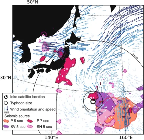
To go deeper into the generation mechanisms of the three seismic phases in terms of location and lateral extent of the sources, we compare the sources of P, SV, and SH waves as observed on September 3, when Ioke was a Category 2 tropical cyclone.
Observations of the three body-wave phases on September 3 allow us to make comparisons of the location and lateral extent of the sources (Fig.3). At 5-s period, sources of P, SV, and SH waves are very close to each other and partially overlap. They are located in the same area in the tail of the typhoon. The source of P waves shows the largest lateral extent, possibly due to the ocean site effect at the source, which is stronger for P than SV waves (“Methods” and Fig. 5). It could also be due to the fact that signals associated with P waves are more energetic and less attenuated at the receivers, yielding to a more efficient back-projection of the source. The region area where P, SV, and SH waves at 5-s period are generated lies between 34 and 5-knots wind-threshold size (see Supplementary Note 1, for more information about typhoon size and windfield). As observed in Fig.2, the source of P waves at 7 s is the only one on September 3 whose energy is mostly concentrated along the coast, highlighting the predominance of a different mechanism. This source is far away from the typhoon and close to the 5-knots wind-threshold size. We observe that the
a) P 5s b) P 7s
c) SV 5s d) SH 5s
Sept: 3 5
Bathymetry slope, degree
Normalized PSD Model Seismic source Percentile 99% 95% Model PSD
Ioke satellite location Sept 3 Sept 5
Fig. 2 Observed and modeled extended seismic sources of typhoon Ioke. Compressional P-wave sources are shown on the top two panels—at (a) 5 s and (b) 7 s—while shear-wave sources are shown on the bottom two panels—(c) SV-wave sources at 5 s, and (d) SH-wave sources at 5 s. Observed seismic sources generated by typhoon Ioke are denoted by contour lines (green contours for sources on September 3 and pink contours for sources on September 5). Modeled P- and SV-wave sources (panelsa–c) represent the pressure PSD in the presence of coastal reflection, modulated by the ocean site effect, and they are shown as colored shadows (blue for sources on September 3 and red for sources on September 5). Observed SH-wave sources in paneld are compared to the slope of the bathymetry.
sources of P, SV, and SH waves at 5-s period are located in the South-East quadrant where the wind speed above the ocean (arrows in Fig.3) is high. On the other hand, the P-wave source at 7-s period is located in a region of low wind speed, further enhancing the predominance of generation mechanisms other than the direct coupling between wind field and surface ocean waves, e.g., ocean-wave coastal reflection.
Sources of secondary microseism shear body waves have been poorly studied so far, and only the location of the maximum energy has been found in a few cases15–19. Retailleau and Gualtieri15 analyzed the P waves generated by typhoon Ioke in
the secondary microseism band. They showed that the seismic sources of P waves follow Ioke’s track as soon as the typhoon gets strong enough and until it dies out as an extratropical storm. Following the theory developed by Haubrich39, they also showed
that there is a cut-off period for the generation of seismic sources that is related to the propagation speed of the typoon. The comparison of the lateral extent and source location of P, SV, and SH waves represents a new observation that sheds light on the generation mechanism of secondary microseisms body waves. The location of the sources and the generation mechanism of secondary microseisms vary significantly with frequency. In the specific case of Typhoon Ioke, we observe the predominance of coastal reflection mechanisms at the long period (T = 7 s) and ocean wave–wave interaction in a deep-water environment at the short period (T= 5 s). We also observe that dispersion of ocean gravity waves alone cannot explain sources close to the coast, both in terms of location and shape. This is evidence that the source area does not necessarily coincide with the generation area, but it is reshaped by the ocean site effect (Supplementary Note 3 and Supplementary Fig. 4). We do not observe any major
bathymetric features, or a particularly thick sedimentary layer, in the source area of SH waves, indicating that they may generate at lateral 3D heterogeneities deep into the Earth.
Those observations are crucial for imaging the Earth’s structure with secondary microseisms. For example, the distance between the centroid of the P-wave sources at 5 s and 7 s (Figs.2and3) is about 15°. Assuming the same location for both of them yields to an error in the travel time and velocity-variation measurements of 30 s and 7.6% for P waves, and 60 s and 6.3% for S waves. If not properly taken into account, these large time shifts may be mis-taken for structural variations, as pointed out by Kedar36.
It is well known that caution is needed to use secondary microseisms as a proxy for assessing the sea state, as the seismic sources of ocean storms do not correspond, in most cases, to the location of the maximum windfield or wave height. On the other hand, the seismic sources of storms are the proxy for identifying the portions of the ocean surface where the non-linear ocean wave–wave interaction occurs efficiently. For example, Retailleau and Gualtieri15 showed that the P-wave
sources associated with typhoon Ioke could not be extracted on thefirst portion of the track, but they could be identified during the extratropical late portion of the track. In both cases, the event was weak, in the process of forming or disappearing, but only in the latter case, the ocean wave–wave interaction occurred efficiently to generate seismic sources. Seismic observations can thus be informative about the sea-state con-ditions for which the wave interactions occur and the depen-dence of the sea state on the wind field blowing over the ocean40,41. Seismic sources of ocean storms have the potential to shed light on the coupling between the ocean and the atmosphere, in addition to the solid Earth.
5 knots
34 knots
Typhoon size Ioke satellite location
Wind orientation and speed Seismic source P 5 sec SH 5 sec SV 5 sec P 7 sec Wind
Fig. 3 Comparison of location and lateral extent of body-wave sources. Map of P-, SV-, and SH-wave source imprints on September 3 at 18:00 UTC. For reference, we show the windfield direction and strength (arrows), and the size of the typhoon defined as the radius that incorporates wind speeds larger than two given thresholds (5 and 34 knots).
Methods
Seismic data analysis. We use the time series recorded between September 2 and 6, 2006 by a network of 129 stations in Southern California (Fig.1a, b), made available by the Southern California Earthquake Center29. The Southern California
network is wide enough to extract P, SV, and SH phases at the selected periods and homogeneous enough to resolve well the source location for the two selected periods of time. We exclude stations in Central California to keep a more homogeneous station distribution.
The data were processed using the python toolboxes numpy, scipy, and Obspy42.
The seismograms are deconvolved with the instrument responses to get ground velocity seismograms. The signals are also downsampled to 2 Hz. The seismograms are then rotated from the (N, E, Z) coordinate system to the (P, SV, T)—where T stands for the transverse-coordinate system (Fig.4). Finally, the seismograms are filtered using a Butterworth band-pass filter in the period bands 4–6 s (Fig.1c), 4.9–5.1 s (Figs.2and3), and 6.9–7.1 s (Figs.2and3).
The back-projection of the seismic source follows the process developed by Retailleau et al.30and Retailleau et al.31and applied on typhoon Ioke by Retailleau
and Gualtieri15. For each 3-h time window analyzed, we perform a grid search of
the potential sources around the typhoon’s satellite location (20∘× 20∘in longitude
and latitude, and a grid spacing of 0. 5∘). For each of these locations, we compute a vespagram10from the data window and extract the energy that corresponds to the
expected arrival slowness predicted in the 1-D Earth model IASP9143for the P, SV,
and SH waves on the P, SV, T components, respectively42,44. Selecting energy
precisely along the expected velocity permits to enhance the useful signal and extract high signal-to-noise ratio information. Thefinal result is a normalized back-projection of the source.
Modeling the sources of P and Sv waves. Secondary microseism sources are generated by the interaction of ocean gravity waves at the surface of the ocean45.
We model the power spectral density (PSD) of the pressurefield generated by ocean wave–wave interaction by using the numerical ocean-wave model WAVE-WATCH III37,46. The PSD of the pressurefield (Pa2/Hz) is defined as
Fpðf ; θ; ϕÞ ¼ ð2πÞ2ρ 2
wg2f E2ðfwÞIðfwÞ
dSðθ; ϕÞ ð1Þ where f is the seismic frequency,θ is the colatitude, ϕ is the longitude, ρwis the
density of the water (assumed constant), g is the gravity acceleration. The ele-mentary surface is dS¼ R2sinθ dθ dϕ, where R is the radius of the Earth. The
factor E(fw) is the PSD of the sea surface elevation (m2/Hz), and I(fw) is the
non-dimensional ocean gravity wave energy distribution as a function of frequency, integrated over the ocean-wave azimuth.
The ocean acts as a waveguide for P waves, which are multiply reflected between the surface of the ocean and the seafloor. At each reflection point at the seafloor, P and SV waves are generated by energy conversion and transmission. The effect of the multiple reflected P waves in the ocean on the wavefield beneath the seafloor is called ocean site effect20. Longuet-Higgins45worked out the ocean site effect on
Rayleigh waves traveling beneath the seafloor. He observed that the ocean site effect is depth- and frequency-dependent. Notably, at T= 5-s period, the fundamental mode of Rayleigh waves is mostly amplified at ~2–3 km water depths, while the first overtone experiences the largest resonance in much deeper oceanic environments, at about 5–6 km (see ref.46, their Fig. 2). For body waves, Gualtieri et al.20found that
there are several peaks of amplification, corresponding to different depths and
Station
E
N
Theta
R
Source
T
a)
b)
Station
Z
inc
Source
R
P
SV
Fig. 4 Rotation to the (P, SV, T) coordinate system. Rotation process to convert the seismograms from the (N, E, Z) coordinate systemfirst to a the (R, T, Z) coordinate system where "Theta" denotes the azimuth and then tob the (P, SV, T) coordinate system where "inc" is the incident angle of the P wave.
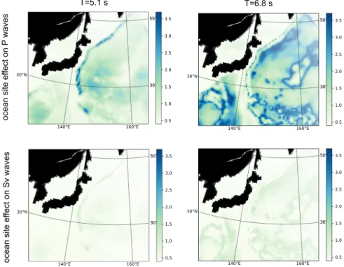
Fig. 5 Ocean site effect on P and Sv waves. Ocean site effect on P (top) and Sv (bottom) waves at 5.1-s (left) and 6.8-s (right) period.
frequencies. At T= 5 s, the acoustic resonance on P and SV waves happens at similar depths, about 2–3 km and 5–6 km (see ref.20, their Fig. 3).
Sources of P and SV waves can be computed by multiplying the PSD of the pressure (Eq. (1)) with the ocean site effect on P and SV waves, respectively. The ocean site effect on body waves varies with frequency, ocean depth, and epicentral distance (ref.20, their Eqs (4) and (12)). We compute the ocean site effect on P and
Sv waves at the same frequencies of the ocean-wave model and considering the epicentral distance between the typhoon location and the average location of the stations (Fig.1b). Figure5shows the ocean site effect on P and S waves at T= 5.1 s and T= 6.8 s. As already observed by Gualtieri et al.20, the ocean site effect on Sv
waves has a similar spatial pattern of the ocean site effect on P waves, but it is characterized by a significantly lower amplitude.
Data availability
The seismic dataset used for this study can be accessed at the Southern California Data Center29through the Obspy toolbox. Center locations of Typhoon Ioke is taken from the Joint Typhoon Warning Center (JTWC) best track dataset47(https://www.metoc.navy.
mil/jtwc/jtwc.html?best-tracks). We used the windfield from the Cooperative Institute for Meteorological Satellite Studies (CIMSS) (http://tropic.ssec.wisc.edu/tropic.canned. php). The output of the ocean-wave model can be found atftp://ftp.ifremer.fr/ifremer/ ww3/HINDCAST/SISMO/. Websites were last accessed on February 16, 2021. Code availability
The codes used to process the seismic data and perform back-projection of the sources are available upon request. To perform synthetic simulations of seismic wave propagation, we used the package SPECFEM3D_GLOBE, which is a freely available code through the Computational Infrastructure for Geodynamics (CIG,https://geodynamics. org/cig/software/specfem3d_globe/, last accessed February 16, 2021).
Received: 8 July 2020; Accepted: 4 March 2021;
References
1. Gutenberg, B. On microseisms. Bull. Seismol. Soc. Am. 26, 111–117 (1936). 2. Webb, S. C. The equilibrium oceanic microseism spectrum. J. Acoustic. Soc.
Am. 92, 2141–2158 (1992).
3. Ebeling, C. W. Inferring ocean storm characteristics from ambient seismic noise: a historical perspective. Advances in Geophysics, Vol. 53 (ed. Dmowska, R.) 1–33 (Elsevier, 2012).
4. Gualtieri, L., Camargo, S. J., Pascale, S., Pons, F. M. & Ekström, G. The persistent signature of tropical cyclones in ambient seismic noise. Earth and Planetary Science Letters 484, 287–294 (2018).
5. Longuet-Higgins, M. S. Can sea waves cause microseisms. Proc. Natl Acad. Sci. USA 306, 74–86 (1953).
6. Backus, M., Burg, J., Baldwin, D. & Bryan, E. Wide-band extraction of mantle p waves from ambient noise. Geophysics 29, 672–692 (1964).
7. ToksöZ, M. N. & Lacoss, R. T. Microseisms: mode structure and sources. Science 159, 872–873 (1968).
8. Haubrich, R. A. & McCamy, K. Microseisms: coastal and pelagic sources. Rev. Geophys. 7, 539–571 (1969).
9. Vinnik, L. P. Sources of microseismicP waves. Pure Appl. Geophys. 103, 282–289 (1973).
10. Rost, S. & Thomas, C. Array seismology: methods and applications. Rev. Geophys. 40, 1008 (2002).
11. Gerstoft, P., Fehler, M. C. & Sabra, K. G. When Katrina hit California. Geophys. Res. Lett. 33, 17 (2006).
12. Zhang, J., Gerstoft, P. & Bromirski, P. D. Pelagic and coastal sources of P-wave microseisms: generation under tropical cyclones. Geophys. Res. Lett. 37, 15 (2010).
13. Sufri, O., Koper, K. D., Burlacu, R. & de Foy, B. Microseisms from superstorm sandy. Earth Planetary Sci. Lett. 402, 324–336 (2014).
14. Fan, W. et al. Stormquakes. Geophys. Res. Lett. 46, 12909–12918 (2019). 15. Retailleau, L. & Gualtieri, L. Toward high-resolution period-dependent
seismic monitoring of tropical cyclones. Geophys. Res. Lett. 46, 1329–1337 (2019).
16. Koper, K. D. & Burlacu, R. Thefine structure of double-frequency microseisms recorded by seismometers in north america. J. Geophys. Res.: Solid Earth 120, 1677–1691 (2015).
17. Gal, M. et al. Deconvolution enhanced direction of arrival estimation using one-and three-component seismic arrays applied to ocean induced microseisms. Geophys. J. Int. 206, 345–359 (2016).
18. Liu, Q. et al. Source locations of teleseismic P, SV, and SH waves observed in microseisms recorded by a large aperture seismic array in China. Earth Planetary Sci. Lett. 449, 39–47 (2016).
19. Nishida, K. & Takagi, R. Teleseismic S wave microseisms. Science 353, 919–921 (2016).
20. Gualtieri, L. et al. Modelling the ocean site effect on seismic noise body waves. Geophys. J. Int. 197, 1096–1106 (2014).
21. Shapiro, N. M., Campillo, M., Stehly, L. & Ritzwoller, M. H. High-resolution surface-wave tomography from ambient seismic noise. Science 307, 1615–1618 (2005).
22. Boué, P., Poli, P., Campillo, M. & Roux, P. Reverberations, coda waves and ambient noise: correlations at the global scale and retrieval of the deep phases. Earth Planetary Sci. Lett. 391, 137–145 (2014).
23. Poli, P., Thomas, C., Campillo, M. & Pedersen, H. A. Imaging the D" reflector with noise correlations. Geophys. Res. Lett. 42, 60–65 (2015).
24. Retailleau, L., Boué, P., Li, L. & Campillo, M. Ambient seismic noise imaging of the lowermost mantle beneath the north atlantic ocean. Geophys. J. Int. 222, 1339–1351 (2020).
25. Sager, K., Boehm, C., Ermert, L., Krischer, L. & Fichtner, A. Sensitivity of seismic noise correlation functions to global noise sources. J. Geophys. Res.: Solid Earth 123, 6911–6921 (2018).
26. Poli, P., Campillo, M. & de Hoop, M. Analysis of intermediate period correlations of coda from deep earthquakes. Earth Planetary Sci. Lett. 477, 147–155 (2017).
27. Tsai, V. C. On establishing the accuracy of noise tomography travel-time measurements in a realistic medium. Geophys. J. Int. 178, 1555–1564 (2009). 28. Lay, T. Deep earth structure: lower mantle and d. Treatise Geophys. 1, 683–72
(2015).
29. SCEDC. Southern California earthquake center. Caltech. Dataset (2013). 30. Retailleau, L., Shapiro, N., Guilbert, J., Campillo, M. & Roux, P. Detecting and
locating seismic events with using USArray as a large antenna. Adv. Geosci. 40, 27–30 (2015).
31. Retailleau, L. et al. Detection and analysis of a transient energy burst with beamforming of multiple teleseismic phases. Geophys. J. Int. 212, 14–24 (2017).
32. Komatitsch, D. & Tromp, J. Spectral-element simulations of global seismic wave propagation—I. Validation. Geophys. J. Int. 149, 390–412 (2002). 33. Komatitsch, D. & Tromp, J. Spectral-element simulations of global seismic
wave propagation—II. Three-dimensional models, oceans, rotation and self-gravitation. Geophys. J. Int. 150, 303–318 (2002).
34. Gualtieri, L., Bachmann, E., Simons, F. J. & Tromp, J. The origin of secondary microseism Love waves. Proc. Natl Acad. Sci. USA 117, 29504–29511 (2020).
35. Kedar, S. et al. The origin of deep ocean microseisms in the North Atlantic Ocean. Proc. Royal Soc. London A: Mathematical, Phys. Eng. Sci. 464, 777–793 (2008).
36. Kedar, S. Source distribution of ocean microseisms and implications for time-dependent noise tomography. Comptes Rendus Geosci. 343, 548–557 (2011).
37. Ardhuin, F., Stutzmann, E., Schimmel, M. & Mangeney, A. Ocean wave sources of seismic noise. J. Geophys. Res.: Oceans 116, C9 (2011). 38. Farra, V., Stutzmann, E., Gualtieri, L., Schimmel, M. & Ardhuin, F.
Ray-theoretical modeling of secondary microseism P waves. Geophys. J. Int. 206, 1730–1739 (2016).
39. Haubrich, R. A. & McCamy, K. Microseisms: coastal and pelagic sources. Rev. Geophys. 7, 539–571 (1969).
40. Janssen, P. The Interaction of Ocean Waves and Wind (Cambridge University Press, 2004).
41. Reichl, B. G., Hara, T. & Ginis, I. Sea state dependence of the wind stress over the ocean under hurricane winds. J. Geophys. Res.: Oceans 119, 30–51 (2014).
42. Krischer, L. et al. ObsPy: a bridge for seismology into the scientific Python ecosystem. Comput. Sci. Discov. 8, 014003 (2015).
43. Kennett, B. & Engdahl, E. Traveltimes for global earthquake location and phase identification. Geophys. J. Int. 105, 429–465 (1991).
44. Crotwell, H. P., Owens, T. J. & Ritsema, J. The TauP toolkit:flexible seismic travel-time and ray-path utilities. Seismol. Res. Lett. 70, 154–160 (1999). 45. Longuet-Higgins, M. S. A theory of the origin of microseisms. Phil. Trans. R.
Soc. Lond. A 243, 1–35 (1950).
46. Gualtieri, L. et al. Modelling secondary microseismic noise by normal mode summation. Geophys. J. Int. 193, 1732–1745 (2013).
47. Chu, J.-H., Sampson, C. R., Levine, A. S. & Fukada, E. The joint typhoon warning center tropical cyclone best-tracks. 1945–2000. Ref. NRL/MR/7540-02, 16, (2002).
Acknowledgements
The dataset was downloaded and processed using python and the seismological com-munity scientific library Obspy42. Python (with the basemap toolbox) and Matlab were used to analyze the results and makefigures. This research used computational resources of the Center for Computational Earth and Environmental Sciences (CEES) at Stanford University.
Author contributions
L.R. performed the seismic data analysis, and L.G. the analytical and numerical modeling. L.R. and L.G. discussed the results, made thefigures, and wrote the paper.
Competing interests
The authors declare no competing interests. Additional information
Supplementary informationThe online version contains supplementary material available athttps://doi.org/10.1038/s41467-021-22231-y.
Correspondenceand requests for materials should be addressed to L.R. or L.G. Peer review informationNature Communications thanks Sharon Kedar, Anya Reading and the other, anonymous reviewer, for their contribution to the peer review of this work.
Reprints and permission informationis available athttp://www.nature.com/reprints
Publisher’s note Springer Nature remains neutral with regard to jurisdictional claims in published maps and institutional affiliations.
Open Access This article is licensed under a Creative Commons Attribution 4.0 International License, which permits use, sharing, adaptation, distribution and reproduction in any medium or format, as long as you give appropriate credit to the original author(s) and the source, provide a link to the Creative Commons license, and indicate if changes were made. The images or other third party material in this article are included in the article’s Creative Commons license, unless indicated otherwise in a credit line to the material. If material is not included in the article’s Creative Commons license and your intended use is not permitted by statutory regulation or exceeds the permitted use, you will need to obtain permission directly from the copyright holder. To view a copy of this license, visithttp://creativecommons.org/ licenses/by/4.0/.
© The Author(s) 2021