GEM/POPs: a global 3-D dynamic model for semi-volatile persistent organic pollutants ? Part 2: Global transports and budgets of PCBs

(1)

HAL Id: hal-00302661

https://hal.archives-ouvertes.fr/hal-00302661

Submitted on 16 Mar 2007

HAL is a multi-disciplinary open access

archive for the deposit and dissemination of sci-entific research documents, whether they are pub-lished or not. The documents may come from teaching and research institutions in France or abroad, or from public or private research centers.

L’archive ouverte pluridisciplinaire HAL, est destinée au dépôt et à la diffusion de documents scientifiques de niveau recherche, publiés ou non, émanant des établissements d’enseignement et de recherche français ou étrangers, des laboratoires publics ou privés.

GEM/POPs: a global 3-D dynamic model for

semi-volatile persistent organic pollutants ? Part 2:

Global transports and budgets of PCBs

P. Huang, S. L. Gong, T. L. Zhao, L. Neary, L. A. Barrie

To cite this version:

P. Huang, S. L. Gong, T. L. Zhao, L. Neary, L. A. Barrie. GEM/POPs: a global 3-D dynamic model for semi-volatile persistent organic pollutants ? Part 2: Global transports and budgets of PCBs. Atmospheric Chemistry and Physics Discussions, European Geosciences Union, 2007, 7 (2), pp.3837-3857. �hal-00302661�

(2)

ACPD

7, 3837–3857, 2007 Global transports and budgets of PCBs P. Huang et al. Title Page Abstract Introduction Conclusions References Tables Figures ◭ ◮ ◭ ◮ Back Close

Full Screen / Esc

Printer-friendly Version Interactive Discussion

EGU Atmos. Chem. Phys. Discuss., 7, 3837–3857, 2007

www.atmos-chem-phys-discuss.net/7/3837/2007/ © Author(s) 2007. This work is licensed

under a Creative Commons License.

Atmospheric Chemistry and Physics Discussions

GEM/POPs: a global 3-D dynamic model

for semi-volatile persistent organic

pollutants – Part 2: Global transports and

budgets of PCBs

P. Huang1, S. L. Gong1,2, T. L. Zhao2, L. Neary3, and L. A. Barrie4 1

Air Quality Research Division, Science & Technology Branch, Environment Canada, 4905 Dufferin Street, Toronto, Ontario M3H 5T4, Canada

2

Department of Chemical Engineering and Applied Chemistry, University of Toronto 200 College Street, Toronto, Ontario, Canada, M5S 3E5, Canada

3

Department of Earth and Space Science and Engineering, York University 4700 Keele Street, Toronto, Ontario, M3J 1P3, Canada

4

Atmospheric Research and Environment Program World Meteorological Organization 7 bis, avenue de la Paix, BP2300, 1211 Geneva 2, Switzerland

Received: 19 January 2007 – Accepted: 3 March 2007 – Published: 16 March 2007 Correspondence to: S. L. Gong (sunling.gong@ec.gc.ca)

(3)

ACPD

Full Screen / Esc

EGU

Abstract

Global transports and budgets of three PCBs were investigated with a 3-D dynamic model for semi-volatile persistent organic pollutants – GEM/POPs. Dominant pathways were identified for PCB transports in the atmosphere with a peak transport flux below 8 km and 14 km for gaseous and particulate PCB28, 4 km and 6 km for gaseous and

5

particulate PCB180. The inter-continental transports of PCBs in the Northern Hemi-sphere (NH) are dominated in the zonal direction with their route changes seasonally regulated by the variation of westerly jet. The transport pathways from Europe and North Atlantic to the Arctic contributed the most PCBs over there. Inter-hemispheric transports of PCBs originated from the regions of Europe, Asia and North America in

10

three different flow-paths, accompanying with easterly jet, Asian monsoon winds and trade winds. PCBs from the Southern Hemisphere (SH) could export into the NH. Ac-cording to the PCB emissions of year 2000, Europe, North America and Asia are the three largest sources of the three PCBs, contributing to the global background con-centrations in the atmosphere and soil and water. Globally, PCB28 in soil and water

15

has become a comparable source to the anthropogenic emissions while heavier PCBs such as PCB153 and 180 are still transporting into soil and water. It is found that lighter PCBs have more long range transport potentials than their heavier counter-parts in the atmosphere.

1 Introduction

20

There is a growing international concern with identifying and managing environmentally persistent substances that are both transported to and deposited into the biosphere of regions far from the place where they were used and released. Atmospheric transport is believed to be the primary mode for conveying persistent substances to these re-mote regions (Wania, 2003), especially for gaseous and insoluble species. POPs vary

25

(4)

ACPD

Full Screen / Esc

EGU their transport and deposition in the environment depends on the unique combination

of persistence and partitioning, which differ considerably from chemical to chemical. These differences in properties translate into differences in chemical fate of various POPs (Mackay et al., 2006).

Previous researches on long range transport (LRT) and deposition of POPs have

5

been mostly limited in assessing the potential for LRT and using simple multimedia models for substances such as the hexachlorocyclohexanes (Wania et al., 1999). These models have been proven extremely useful as an exploring and policy tool in demonstrating the “grasshopper” and “cold condensation” effects and in examining movement over the globe on time scales of several decades in a steady state mode

10

to investigate the partitioning behaviors of POPs or in a dynamic mode to simulate the environmental fate of a compound. Due to the poor spatial and temporal resolutions of these models, a source–receptor relationship can hardly be inferred quantitatively for any specific geographical regions. To overcome the limitation of box-type models, dynamical 3-D models have been developed to describe the atmospheric transport

15

of POPs on both regional (Ma et al., 2003; van Jaarsveld et al., 1997), hemispheric (Hansen et al., 2005; Malanichev et al., 2004) and global scales (Gong et al., 2007; Koziol and Pudykiewicz, 2001; Semeena and Lammel, 2005). Transport and deposi-tion patterns of various POPs have been investigated with respect to factors such as the climate fluctuations. One thing that lacks in these 3-D model studies was the

inves-20

tigation of the budgets and deposition patterns of inter-continental transports of various semi-volatile POPs. The quantitative relationship between the emissions in one region and the environmental levels in another region hundreds and thousands of kilometers away was not properly addressed under various partitioning conditions.

As described in the previous paper (Gong et al., 2007), a 3-D global POPs

trans-25

port model with a dynamic aerosol module (GEM/POPs) has been developed to sim-ulate the transport, deposition and partitioning of semi-volatile POPs in the atmo-sphere. Comparisons of GEM/POPs results with observations have revealed that the GEM/POPs can reasonably simulate the atmospheric distributions of three

(5)

typi-ACPD

Full Screen / Esc

EGU cal PCBs from volatile (PCB28) to semi-volatile (PCB153 and PCB180) species for

their ranges and seasonal variations of the atmospheric concentrations, which allows the further investigation of PCB global transport patterns and budgets. This paper is to present the current status of atmospheric PCBs in terms of their reservoirs, inter-continental transports and deposition patterns in an effort to comprehensively

under-5

stand the nature of current PCBs.

2 GEM/POPs essentials

The full details of development of GEM/POPs by a Canadian community effort are given in a previous paper (Gong et al., 2007). This section briefly reviews the key com-ponents of the modeling system. Four major function blocks form the GEM/POPs

sys-10

tem: transport, exchange/emission, particulate and gaseous processes. The transport of POPs is carried out atmospherically by the Global Environmental Multiscale (GEM) model (C ˆot ´e et al., 1998) developed at MSC (Meteorological Service of Canada) for weather forecasting applications and oceanically by prescribed ocean currents and a ocean tracer transport module. The exchanges of POPs between atmosphere and

wa-15

ter/soil as well as the anthropogenic emission provide GEM/POPs the net fluxes into the atmosphere where they are engaged into transport, gaseous and particulate pro-cesses. Within the particulate processes, an on-line aerosol module CAM (Canadian Aerosol Module) (Gong et al., 2003) computes dynamically the aerosol surface areas from five major aerosol components: sea-salt, sulphate, black carbon, organic carbon

20

and soil dust. The dry and wet removals of particle-bound PCBs are also treated in this block, the downward fluxes of which are added to the soil and water reservoirs, re-spectively. Finally, the degradation by OH, gas-particle partition as well as the dry and wet removals of gaseous PCBs is handled in the gaseous phase block. The deposition fluxes of gaseous phase PCBs are dynamically tracked in soil and water reservoirs as

25

(6)

ACPD

Full Screen / Esc

EGU

3 Global transports of PCBs

The global transports of PCBs are investigated based on the analyses of transport flux which is calculated in zonal and meridional components by multiplying PCB-concentration and zonal/meridional wind velocity components. Therefore positive (neg-ative) transport flux components of PCBs indicate eastward (westward) transport in

5

zonal direction or northward (southward) transport in meridional direction depending on the directions of wind velocity components. As a vector variable, transport flux is used to estimate the amount and direction of PCB transport in this section.

3.1 Global transport patterns

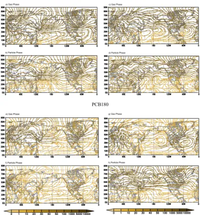
Figure 1 shows the meridional cross-section of zonal and meridional components

10

of globally mean PCB-transport fluxes averaged over the year 2000. Climatologi-cally, west winds prevail with the westerly jets in the mid-latitudes of both NH and SH for all seasons. Therefore, it could be expected that the zonal transports of both volatile (PCB28) and semi-volatile (PCB180) PCBs in the eastward direction over the mid-latitudes of both hemispheres are globally strongest considering the major

PCB-15

sources there, although the minor westward transports of PCBs occurred in the east-erlies over the low- and high-latitudes. It can also be seen that most PCBs were trans-ported in the troposphere. In the NH, the zonal PCB-transports peaked below 4 km for the gaseous PCB180, 6 km for the particulate PCB180 particles, 8 km for the gaseous PCB28 and 14 km for particulate PCB28 with the transport centers around 50◦_{N. In}

20

the SH, the eastward transports centered around 40◦_{S peaked at the higher altitudes}

with a lower strength than in the NH, primarily due to long range transport from the source regions in the NH (Figs. 1a–d). The lighter PCB (i.e. PCB28) is transported with stronger westerlies at higher layers than the heavier PCB (i.e. PCB180), which implied that the lighter PCB exhibits a more LRT-potential than the heavier PCB. The

25

globally averaged transport flux components in the meridional direction indicated that PCBs from the regions at the latitudinal range 40–50◦_{N could transport northwards}

(7)

ACPD

Full Screen / Esc

EGU into the arctic region and southwards into the low-latitudes, and cross equator into

the SH (Figs. 1e–h). The meridional transports of PCBs were also mostly limited in the troposphere at the same altitudes with the zonal transports excepting the particu-late PCB28. Compared to the semi-volatile PCB180, more particles of PCB28 could be volatized into the gas phase proportionally to the air temperature. Therefore, the

5

pattern of meridional transports for the particulate PCB28 was formed with the major transport layers descending from the warm low-latitudes to the cold high-latitudes in the both Hemispheres. In the NH, the most PCB28-particles transported northwards from mid- to high-latitudes below 8 km, southwards from mid- to low-latitudes between 6 km and 12 km, and across the equator at the altitudes of 10 km–14 km (Fig. 1h). It is also

10

found in Fig. 1 that more gaseous PCB28 than particulate PCB28 were involved in LRT in both zonal and meridional directions, while more particulate PCB180 than gaseous PCB180 were engaged in LRT. These differences in the PCB transport amounts and layers of lighter PCB28 and heavier PCB180 are related with their magnitude of emis-sion, chemical degradation, deposition and the gaseous and particulate processes.

15

3.2 Inter-continental transports in NH

Based on the above analysis of the PCB transport layers, the transport fluxes averaged from surface to 8 km for gaseous PCB28, to 14 km for the particulate PCB28, to 4 km for the gaseous PCB180 and to 6 km for the particulate PCB180 were used to further describe the global transport patterns and their seasonal variations with the streamline

20

fields in Figs. 2 and 3 to more comprehensively understand the global transports. Closely associated with the atmospheric general circulation especially with west-erly wave in the mid-latitudes, the inter-continental transports of PCBs in the NH are dominant in the eastward direction along the westerlies (Fig. 2). The inter-continental transport routes changed from the more meridinal structures in winter and spring to

25

the more zonal structures in summer and autumn, associated with the seasonal evo-lution of trough and ridge system in westerly wave. In winter the meridional transport pattern was well built up with three ridges over the regions: 1) from central Asia to

(8)

ACPD

Full Screen / Esc

EGU Siberia, 2) between Eastern Pacific and western North America and 3) of western

At-lantic and with two troughs: 1) from East Asia to western Pacific and 2) over eastern North America (Figs. 2a–b, 2e–f). The strongest ridge from central Asia to Siberia brought PCBs from Europe across the high latitudes and the arctic into East Asia, North Pacific and even North America. The PCB-sources in Europe seem to be the

5

most important for the inter-continental transports in the NH. The stream jets of PCB-transports in the two trough regions carried PCBs from Eurasian continent to Pacific and from North America to Atlantic Ocean (Figs. 2a–b, 2e–f). The seasonal variations of stream jets are featured with their centre location at 35◦_{N in winter (Figs. 2a–b, 2e–}

f), 40–45◦_{N in spring/autumn and 50}◦_{N in summer (Figs. 2c–d, 2c–d). In summer the}

10

zonal PCB-transport pattern was most clearly developed with the weakest trough and ridge system in the westerlies of the NH, especially for PCB28 in the middle and upper troposphere (Figs. 2c–d). For the heavier PCB180-transports in the lower troposphere with the stronger effects from the topography, the inter-continental transport routes with the less zonal and less streamline structures could also present a lower potential for

15

LRT (Figs. 2e–h).

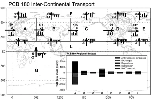
Figures 3a and 4a further quantify the transport mass of PCB28 and PCB180 in year 2000. To facilitate the discussions, the globe is divided into 8 regions, repre-senting the Europe, Asia, North Pacific, North America, Atlantic, Arctic, SH and NH low-latitude, respectively as shown in Figs. 3 and 4. For European region , the sum

20

of imported gaseous and particulate PCBs was 4358 kg and 71 kg for PCB28 (Fig. 3a) and PCB180 (Fig. 4a), respectively, while those two congeners exported from the Euro-pean region totalled 26 491 kg and 297 kg, that confirmed that Europe was the largest PCB-sources for LRT. From Europe, 20 276 kg of total exported PCB28 and 192 kg of total exported PCB180 transferred eastwards to Asian region, 5914 kg of PCB28 and

25

89 kg of PCB180 northwards into the Arctic region, reflecting a higher LRT potential for PCB28 than for PCB180. In spite of the third largest emitter of PCBs in the world (Table 1), Asian region was a sink for PCBs with an annual PCB28 (PCB180) import of 20 276 kg (213 kg) and an export of 13 112 kg (121 kg). Relative to the total PCB28

(9)

ACPD

Full Screen / Esc

EGU (PCB180) imported into each region, the eastward transports of PCBs contributed

about 100% (90%) to Asian region from Europe, 99% (95%) to North Pacific region from Asia, 63% (80%) to North American region from North Pacific and 99% (97%) to Atlantic region from North America. This further confirmed that the eastward LRT of PCBs is dominant in the mid-latitude of NH. Situated in the downwind of Asia and

5

North America, North Pacific and Atlantic were also the major sinks for both PCB28 and PCB180 during their LRT. Corresponding with the ridges of westerly wave in the NH, the meridional transports across the northern boundaries (Arctic Circle) were also im-portant especially for Europe, North America and Atlantic with the substantial exports and imports (Figs. 3a and 4a). These were the alternative pathways of inter-continental

10

transports across Arctic besides the zonal transports. The transport fluxes of PCB28 and PCB180 in winter, spring, summer and fall were also shown in the bar charts of Figs. 3a and 4a. There existed seasonal variations of PCB-transports for each region but no general conclusions can be drawn.

3.3 Transport to the Arctic

15

Governed by the seasonal changes in westerly wave with trough and ridge in mid-and high-latitudes the pattern of PCB-transports into the arctic presented the obvious sea-sonal variations. Corresponding with the seasea-sonal position and strength of the westerly ridges, the PCBs entered the Arctic Circle (66.50◦_{N) northwards in winter/spring over}

three following areas: 1) East Europe to central Asia, 2) western Pacific and 3) eastern

20

Atlantic (Figs. 2a–b and 2e–f), in summer over two following regions: 1) from Europe to western Asia and 2) from eastern North America to western Atlantic (Figs. 2c–d and 2g–h) as well as in autumn with four entrances: 1) from Eastern Atlantic to West-ern Europe, 2) over central Asia, 3) north Pacific and 4) from eastWest-ern North America to western Atlantic. Annually, the Arctic received 5914 kg (89 kg) of PCB28 (PCB180)

25

from European region, 1217 kg (26 kg) from North Atlantic region and exported 2413 kg (8.7 kg) of PCB28 (PCB180) to North American region and 21.4 kg PCB180 to Asian re-gion. The transports from Europe to Arctic and from North Atlantic (the source in North

(10)

ACPD

Full Screen / Esc

EGU America) to the Arctic contributed the most PCBs. As a pure sink of global PCBs,

the Arctic region had a net import of 5214 kg (80 kg) of PCB28 (PCB180) (Figs. 3a and 4a). It was also found that not only more gaseous PCB28 transported from Eu-rope into the Arctic than particulate PCB28 but also they crossed the Arctic Circle in opposite directions from the northern boundaries of Europe, Asia and North Pacific

5

(Fig. 3a). This can be explained by the vertical meridional circulation structures that are responsible for the transports of gaseous PCB28 in middle troposphere and partic-ulate PCB28 in upper troposphere. Compared to the eastward transports, PCB180 had strong meridinal transport components to carry more PCBs from directly the sources in Europe and North America into Arctic than PCB28 (Figs. 2a–d, 3a and 4a), because

10

PCB180-transports were limited in the lower atmospheric layers with the more impacts of surface.

3.4 Transport between NH and SH

In the NH, most of PCBs emitted in Europe, South/East Asia and North America (Ta-ble 1). PCBs originated from these regions transported between NH and SH across the

15

equator in the different flow-paths. For PCB28 (Fig. 2a–d) and PCB180 (Figs. 2e–h), there were three pathways of cross equatorial transports: 1) southwards from Europe into the easterly jet over tropical Africa and Atlantic for the whole year, 2) southwards from East and South Asia with winter monsoon to the SH and northwards with summer monsoon from the SH to South and East Asia and 3) from North America around the

20

subtropical High into trade winds in the tropics. The transport directions of pathway 2 from South/East Asia to tropical Indian Ocean and west Pacific were seasonally shifted accompanying Asian summer and winter monsoon. It is interesting that the summer-time PCBs in the low and middle troposphere could transport from the SH to NH across the equator. Due to the most transports of PCB28 particles in the upper troposphere

25

in the tropics (Fig. 1h), their cross equatorial transports presented the opposite direc-tions with the gaseous PCB28’s in the most tropical regions especially in winter and summer (Figs. 2a–d), corresponding to the meridional and zonal circulations between

(11)

ACPD

Full Screen / Esc

EGU lower and upper troposphere in the tropics. The opposite directions of these cross

equatorial transports for PCB28 gas and particles are also seen from their annual to-tal gas of 148 kg from NH to SH and particles of 79 kg from Southern to NH in 2000 (Fig. 3a). The seasonal shift of the cross equatorial transports between the NH and SH for both gaseous and particulate PCB28 were obviously demonstrated, especially

5

between summer and winter (Figs. 2a, b and 3a), which implied that PCBs from the SH could enter and affect the NH under some favourite conditions. As the passages of the cross equatorial transports from the PCB-sources in the northern mid-latitudes, the northern lower latitude region gained 1729 kg (53 kg) from the mid-latitudes and exported 69 kg (8 kg) of total PCB28 (PCB180) to the SH. Both regions L and G were

10

the receptor-regions of global PCB-transports (Figs. 3a and 4a).

4 Global budgets of PCBs

4.1 Anthropogenic emissions

According to Breivik et al. (2002) by a mass balance approach, the global annual emis-sions of the three PCB congeners of 28, 153 and 180 simulated in this study are 54 663,

15

12 099 and 3104 kg, respectively. Redistributed in each country by its population dis-tribution, the global 1◦

×1◦ grid emissions were produced. Table 1 shows the regional contribution of three PCBs to the total global emissions. It is obvious that industrial-ized regions of the NH contribute majority of the anthropogenic PCBs with about 65% contributions from Europe, 15% from North America and 10% from Asia. It should be

20

noted that only the high emission scenario of the three estimates provided in Breivik et al. (2002) was employed in this study.

4.2 Soil and water fluxes to the atmosphere

The soil and water fluxes emitted to the atmosphere were estimated by two exchange modules in GEM/POPs (Gong et al., 2007) based on the soil and water

(12)

ACPD

Full Screen / Esc

EGU tions of the three PCBs in this study. Because of the uncertainties associated with

the estimates of soil and water concentrations, these values are also subject to large uncertainties. However, given the fact that these soil and water PCB concentrations used in our previous studies have yielded reasonable atmospheric PCB concentra-tions compared with observaconcentra-tions, estimates of the fluxes with these soil and water

5

concentrations could give an order of magnitude approximation. Table 1 shows the three categories of emissions for PCB28, 153 and 180: anthropogenic, soil and water. A positive value in the table indicates an upward flux to the atmosphere and vice versa. The estimated fluxes of three PCBs from soil and water for the SH are all negative, indicating that the entire southern eco-system is still a net sink for global PCBs. This is

10

also true for all the water and soil compartments in the lower latitude region. In other regions, the directions of PCB exchanges depend on the regional soil and water con-centrations and PCB congeners. The sign of the exchange fluxes between soil/water and atmosphere is determined by the relative magnitudes of the fugacity for a chemi-cal concerned in each media (Mackay, 2001). Simulated results show that fugacity of

15

PCB28 in most northern soil and water compartments is larger than that in the atmo-sphere, which results in a net flux of PCB28 from soil and water to the atmosphere. The sum of soil and water emission fluxes to the atmosphere for PCB28 had reached or surpassed the same magnitude as the anthropogenic emissions. The ratio of soil and water to anthropogenic fluxes of PCB28 for year 2000 was 0.74 in Europe, 1.27 in

20

Asia, 0.67 in North America and 2.57 in the Arctic. This indicates that PCB28 in soil and water has become a net source for PCBs after years of depositions from the past usage.

For most regions, anthropogenic emissions are still the dominant source of heav-ier PCBs (PCB153 and 180) while soil and water compartments continue receiving

25

PCBs from the atmosphere except for soil in North America and the Arctic for PCB180 (Table 1).

(13)

ACPD

Full Screen / Esc

EGU 4.3 Source and receptor regions of global PCBs

In addition to the inter-continental transport fluxes, Figures 3b and 4b also show the budget information of PCB28 and 180 for each region to investigate the mass transfers due to anthropogenic emissions and air-surface exchange processes, and the removal processes. For the convenience of the analysis, the total global emission (TGE) for

5

PCB28, PCB153 and PCB180 is defined as the sum of its anthropogenic emissions plus the upward fluxes from water/soil to the atmosphere for year 2000 with its regional counter-part as Ems (kg/yr). The regional removal of each congener consists of two contributions: gas-phase reactions with OH (L_decay, kg/yr) and dry and wet removal processes of gases and particles in atmosphere (Ldepo, kg/yr). Trans (kg/yr) is the net

10

mass transported through the boundaries of each region with a positive value as a net import into the region and vice versa. Table 2 presents the Ems, percentage of Ems

L_depo, L_decayand Transof three PCBs over each region with respect to the TGE.

T_rans% for regions A and D were negative for all three congeners (Table 2), indi-cating that they were source regions and exported all three PCBs in year 2000 to

15

other regions where T_rans% were positive. According to the modeling results, TGE was 96 453 kg, 12 100 kg and 3330 kg for PCB28, PCB153 and PCB180, respectively, among which Europe and North America together contributed 73 858 kg, 9463 kg and 2678 kg. T_rans% for PCB28, PCB153 and PCB180 over the two regions were –28%, –10% and –15% of TGE, which are translated into a net export of 27 277 kg, 1214 kg

20

and 489 kg of PCB28, PCB153 and PCB180 to other regions (Table 2, Figs. 3b, 4b). It should be noted that Asia, the third biggest contributor of PCBs into the atmosphere, was a receptor as its Trans% > 0 for all three congeners. Total Trans% over Asia, Pacific,

Atlantic and Arctic for PCB28, PCB153 and PCB180 are 26%, 9% and 13% of TGE, respectively (Table 2). This indicates that the four regions are the primary receptors

25

of PCBs in the globe. Whereas regions G and L have considerable large area, but as receptors, they only receive very small amount of masses from other regions (Table 2) and therefore slightly affected by the northern source regions.

(14)

ACPD

Full Screen / Esc

EGU 4.4 Removals of different PCB congeners

According to Table 2, 68%, 89% and 91% of PCB28, PCB153 and PCB180 emitted from European region were removed in the area. For PCB28, 91% of the removal was due to the reaction with OH in the atmosphere and only 9% was due to depositions. However, for heavier congeners of PCB153 (PCB180), 94% (97%) removals in region

5

A were due to wet and dry depositions with the remaining percentages by gaseous PCB reactions with OH in the atmosphere. This phenomenon existed in all regions as well (Table 2 and Figs. 3b, 4b). On the global scale, the removal of PCB28 by reaction with OH radicals was much larger than the sum of loss of PCB153 and PCB180 by OH reaction (Table 2).

10

PCBs’ removal pattern over Pacific and Atlantic area greatly depends on the different LRT potential of PCBs. The area of Atlantic is almost as half as that of Pacific, but removals of PCB180 in Atlantic were as twice as those in Pacific (Table 2, Figs. 3b, 4b). Yet for PCB28, the removals were proportional to area of the two regions (Figs. 3b, 4b). This once again demonstrates the difference of LRT potential of various PCBs with

15

lighter PCBs more uniformly distributed around globe and heavier PCBs limited close to their source regions.

This study is a first attempt with a 3-D global POPs transport model to study the budgets and inter-continental transports of various PCBs. The results have shown that GEM/POPs could properly address behaviors of PCBs in atmosphere. More features

20

and longer simulations of PCBs are recommended to study historical global fate of PCBs in the future.

Acknowledgements. The authors wish to thank CFCAS (The Canadian Foundation for Climate

and Atmospheric Sciences) for its partial finical support for this research through the NW AQ MAQNet Grant.

(15)

ACPD

Full Screen / Esc

EGU

References

Breivik, K., Sweetman, A., Pacyna, J. M., and Jones, K. C.: Towards a global historical emission inventory for selected PCB congeners – a mass balance approach 2. Emissions, Sci. Total Environ., 290, 199–224, 2002.

C ôt é, J., Gravel, S., M éthot, A., Patoine, A., Roch, M., and Staniforth, A.: The operational 5

CMC-MRB Global Environmental Multiscale (GEM) model: Part I – Design considerations and formulation, Mon. Wea. Rev., 126, 1373–1395, 1998.

Gong, S. L., Barrie, L. A., Blanchet, J.-P., Salzen, K. v., Lohmann, U., Lesins, G., Spacek, L., Zhang, L. M., Girard, E., Lin, H., Leaitch, R., Leighton, H., Chylek, P., and Huang, P.: Canadian Aerosol Module: A size-segregated simulation of atmospheric aerosol processes 10

for climate and air quality models 1. Module development, J. Geophys. Res., 108, 4007, doi:10.1029/2001JD002002, 2003.

Gong, S. L., Huang, P., Zhao, T. L., Sahsuvar, L., Barrie, L. A., Kaminski, J. W., Li, Y. F., and Niu, T.: GEM/POPs: A Global 3-D Dynamic Model for Semi-volatile Persistent Organic Pollutants 1. Model description and evaluations, Atmos. Chem. Phys. Discuss., 7, 3397–3422, 2007, 15

http://www.atmos-chem-phys-discuss.net/7/3397/2007/.

Hansen, K. M., Christensen, J. H., Brandt, J., Frohn, L. M., and Geels, C.: Modelling atmo-spheric transport persistent organic pollutants in Northern Hemisphere with a 3-D dynamical model: DEHM-POP, Atmos. Chem. Phys., 4, 1339–1369, 2005.

Koziol, A. S. and Pudykiewicz, J. A.: Global-scale environmental transport of persistent organic 20

pollutants, Chemosphere, 45, 1181–1200, 2001.

Ma, J., Daggupaty, S., Harner, T., and Li, Y.-F.: Impacts of Lindane usage in the Canadian prairies on the Great Lakes ecosystem, 1. Coupled atmospheric transport model and mod-eled concentrations in air and soil, Envion. Sci. Technol., 37(17), 3774–3781, 2003.

Mackay, D.: Multimedia Environmental Models: The Fugacity Approach. CRC Press, New York, 25

2001.

Mackay, D., Webster, E., and Gouin, T.: Partitioning, Persistence and Long-Range Transport, in: Chemicals in the Environment: Assessing and Managing Risk, edited by: Hester, R. E. and Harrison, R. M., Royal Society of Chemistry, Cambridge, UK, 2006.

Malanichev, A., Mantseva, E., Shatalov, V., Strukov, B., and Vulykh, N.: Numerical evaluation 30

of the PCBs transport over the Northern Hemisphere. Environ. Pollut., 128, 279–289, 2004. Semeena, V. S. and Lammel, G.: The significance of the grasshopper effect on the

(16)

at-ACPD

Full Screen / Esc

EGU

mospheric distribution of president organic substances, Geophys. Res. Lett., 32, L07804, doi:10.1029/2004GL022229, 2005.

van Jaarsveld, J. A., van Pul, W. A. J., and de Leeuw, F. A. A. M.: Modelling transport and de-position of persistent organic pollutants in the European region, Atmos. Environ., 31, 1011– 1024, 1997.

5

Wania, F.: Assessing the potential of persistent organic chemicals for long-range transport and accumulation in polar regions, Environ. Sci. Technol., 37, 1344–1351, 2003.

Wania, F., Mackay, D., Li, Y.-F., Bidleman, T. F., and Strand, A.: Global chemical fate of alpha-hexachlorocyclohexane. 1. Evaluation of a global distribution model, Environ. Toxicol. Chem., 18, 1390–1399, 1999.

(17)

ACPD

Full Screen / Esc

EGU Table 1. Relative Strength of Three PCBs for year 2000 (kg).

Media Europe Asia Pacific North Atlantic Arctic SH Low Total America Latitude PCB28 Anthropogenic 33 644.40 7269.09 210.47 9260.15 92.28 259.92 1985.06 1942.38 54 663.75 Soil 24 281.40 9232.98 68.83 6170.20 32.48 1587.36 –612.17 –135.80 40 625.28 Water 481.49 25.21 307.93 18.73 498.94 –920.33 –128.87 –59.96 223.14 PCB153 Anthropogenic 7974.51 1178.72 36.19 1488.72 37.83 37.28 683.97 662.75 12 099.96 Soil –4,252.65 –802.00 –25.24 –528.09 –7.81 –45.60 –484.97 –334.57 –6480.93 Water –232.87 –24.98 –18.93 –45.86 –42.83 –5.47 –34.32 –29.74 –435.00 PCB180 Anthropogenic 1974.27 251.83 9.76 481.84 10.57 7.14 187.50 181.08 3104.01 Soil –723.66 –132.76 –2.81 236.98 1.90 5.46 –144.88 –111.40 –871.17 Water –46.03 –4.69 –4.78 –14.98 –13.78 –1.02 –6.95 –12.48 –104.71

(18)

ACPD

Full Screen / Esc

EGU Table 2. Regional PCB Budgets.

Region PCB28 PCB153 PCB180 Ems [kg/yr] Ems % Ldepo % Ldecay % Trans % Ems [kg/yr] Ems % Ldepo % Ldecay % Trans % Ems [kg/yr] Ems % Ldepo % Ldecay % Trans % A 58408.20 60.56 3.92 37.51 –22.95 7974.51 65.91 55.18 3.75 –7.24 1974.27 59.28 52.48 1.36 –6.79 B 16528.77 17.14 1.77 21.21 7.43 1178.72 9.74 10.85 0.83 2.50 251.83 7.56 10.04 0.25 2.71 C 587.32 0.61 2.37 4.57 7.80 36.19 0.30 1.57 0.14 1.65 9.76 0.29 2.18 0.06 2.23 D 15449.87 16.02 1.06 10.46 –5.33 1488.72 12.30 8.67 1.22 –2.79 703.86 21.13 12.50 1.34 –7.90 E 623.75 0.65 1.89 3.65 5.85 37.83 0.31 2.85 0.32 2.79 10.57 0.32 5.58 0.21 5.68 F 927.22 0.96 1.28 4.20 5.41 37.28 0.31 1.68 0.06 1.72 11.59 0.35 2.52 0.02 2.46 G 1985.06 2.06 1.09 1.84 0.07 683.97 5.65 5.58 0.33 0.31 187.50 5.63 5.93 0.09 0.24 L 1942.38 2.01 0.82 4.22 1.72 662.75 5.48 5.72 0.87 1.07 181.08 5.44 6.79 0.29 1.37

(19)

ACPD

Full Screen / Esc

Printer-friendly Version Interactive Discussion EGU PCB 180 zonal components PCB 28 a) b) c) d) e) f) g) h) PCB 180 meridional components PCB 28

Fig. 1. The meridional cross-section of globally mean PCB-transport fluxes (ng km−2_s−1₎ av-eraged over the year 2000 with the zonal components of (a) gaseous PCB180, (b) gaseous PCB28, (c) particulate PCB180, (d) particulate PCB28 and the meridional components of (e) gaseous PCB180, (f) gaseous PCB28, (g) particulate PCB180 and h) particulate PCB28. The vertical coordinates are for the altitude (m) from surface.

(20)

ACPD

Full Screen / Esc

Printer-friendly Version Interactive Discussion EGU PCB28 Winter Summer a) Gas Phase b) Particle Phase c) Gas Phase d) Particle Phase PCB180 e) Gas Phase f) Particle Phase g) Gas Phase h) Particle Phase

Fig. 2. Seasonally mean streamlines of PCB28-transport fluxes (×20 ng km−2_s−1_{) averaged} below the limited vertical layers in winter for (a) gas and (b) particles, and in summer for (c) gas and (d) particles. The limited vertical layers are at 8 km for gaseous PCB28 and 14 km for particulate PCB28. Seasonally mean streamlines of PCB180-transport fluxes (ng km−2_s−1₎ averaged below the limited vertical layers in winter (e) for gas and (f) for particles and in summer

(g) for gas and (h) for particles. The limited vertical layers are at 4 km for gaseous PCB180 and

(21)

ACPD

Full Screen / Esc

Printer-friendly Version Interactive Discussion EGU PCB 28 Inter-Continental Transport A B D E F G L C 1600 2758 2498 17778 281 -582 -73 5987 2254 9941 -178 -246 -248 741 1396 2644 -227 -402 111 -108 2209 9240 54 -198 -736 -1677 14 -245 215 1002 79 -148 PCB028 Regional Budget A B C D E F G L P C B T o ta l m a s s [k g /y r] -80000 -60000 -40000 -20000 0 20000 40000 60000 80000 Anthropogenic Emissions Exchanges Depositions Degradation Net Transport

Fig. 3. (a) Inter-continental transports of PCB28. The transport masses at four sides of each

region are marked with a pair of numbers (particulate/ gaseous PCBs in kg yr−1_{), an arrow and} a bar chart. A positive or negative number indicates the same or opposite transport directions as the arrows. The bar charts beside each arrow show the PCB transport masses of PCB particles (black bars) and gas (gray bars) through region boundary in winter, spring, summer and fall. (b) PCB28 regional budget (kg yr−1_).

(22)

ACPD

Full Screen / Esc

Printer-friendly Version Interactive Discussion EGU PCB 180 Inter-Continental Transport A B C D F G E L 69 2 171 21 -7 -9 79 10 105 8 -6 -2 - 21 -0.4 36 -1 -5 -3 -5 0.4 247 49 -6 -4 -9 0.3 -4 -7 25 1 -6 -2 PCB180 Regional Budget A B C D E F G L PC B T o ta l m a s s [k g /y r] -3000 -2000 -1000 0 1000 2000 3000 Anthropogenic Emissions Exchanges Depositions Degradation Net Transport