Validation of the Atmospheric Chemistry Experiment (ACE) version 2.2 temperature using ground-based and space-borne measurements

HAL Id: hal-00328559

https://hal.archives-ouvertes.fr/hal-00328559

Submitted on 10 Oct 2008

HAL is a multi-disciplinary open access

archive for the deposit and dissemination of

sci-entific research documents, whether they are

pub-lished or not. The documents may come from

teaching and research institutions in France or

abroad, or from public or private research centers.

L’archive ouverte pluridisciplinaire HAL, est

destinée au dépôt et à la diffusion de documents

scientifiques de niveau recherche, publiés ou non,

émanant des établissements d’enseignement et de

recherche français ou étrangers, des laboratoires

publics ou privés.

(ACE) version 2.2 temperature using ground-based and

space-borne measurements

R. J. Sica, M. R. M. Izawa, K. A. Walker, C. Boone, S. V. Petelina, P. S.

Argall, P. Bernath, G. B. Burns, Valéry Catoire, R. L. Collins, et al.

To cite this version:

R. J. Sica, M. R. M. Izawa, K. A. Walker, C. Boone, S. V. Petelina, et al.. Validation of the

Atmo-spheric Chemistry Experiment (ACE) version 2.2 temperature using ground-based and space-borne

measurements. Atmospheric Chemistry and Physics, European Geosciences Union, 2008, 8 (1),

pp.35-62. �10.5194/acp-8-35-2008�. �hal-00328559�

www.atmos-chem-phys.net/8/35/2008/ © Author(s) 2008. This work is licensed under a Creative Commons License.

Chemistry

and Physics

Validation of the Atmospheric Chemistry Experiment (ACE) version

2.2 temperature using ground-based and space-borne measurements

J. C. Lambert12, E. J. Llewellyn5, G. L. Manney17,18, I. S. McDermid19, K. Mizutani20, Y. Murayama20, C. Piccolo21, P. Raspollini22, M. Ridolfi23, C. Robert9, W. Steinbrecht24, K. B. Strawbridge13, K. Strong4, R. St ¨ubi25, and

B. Thurairajah10

1_{Department of Physics and Astronomy, The University of Western Ontario, London, Ontario, Canada} 2_{Department of Earth Sciences, The University of Western Ontario, London, Ontario, Canada}

3_{Department of Chemistry, University of Waterloo, Waterloo, Ontario, Canada} 4_{Department of Physics, University of Toronto, Ontario, Canada}

5_{Institute of Space and Atmospheric Studies, University of Saskatchewan, Saskatoon, Canada} 6_{Department of Physics, La Trobe University, Victoria, Australia}

7_{Department of Chemistry, University of York, UK}

8_{Ice, Ocean, Atmosphere and Climate Program, Australian Antarctic Division, Kingston, Tasmania, Australia} 9_{Laboratoire de Physique et Chimie de l’Environnement, CNRS - Universite d’Orleans, France}

10_{Geophysical Institute and Atmospheric Sciences Program, University of Alaska Fairbanks, Alaska} 11_{Columbus Technologies Inc., Pasadena, California, USA}

12_{Institut d’Aeronomie Spatiale de Belgique (IASB-BIRA), Brussels, Belgium}

13_{Science and Technology Branch, Environment Canada, CARE, Egbert, Ontario, Canada} 14_{Leibniz-Institute of Atmospheric Physics, K¨uhlungsborn, Germany}

15_{Service d’A´eronomie, Institut Pierre Simon Laplace-UVSQ, Verrires-le-Buisson, France} 16_{Finnish Meteorological Institute – Arctic Research Centre, Sodankyl¨a, Finland}

17_{Jet Propulsion Laboratory, California Institute of Technology, Pasadena, California, USA} 18_{New Mexico Institute of Mining and Technology, Socorro, New Mexico, USA}

19_{Jet Propulsion Laboratory, California Institute of Technology, Table Mountain Facility, Wrightwood, California, USA} 20_{National Institute of Information and Communications Technology, Tokyo, Japan}

21_{Department of Atmospheric, Oceanic and Planetary Physics, Clarendon Laboratory, Oxford, UK}

22_{Istituto di Fisica Applicata “Nello Carrara” (IFAC) del Consiglio Nazionale delle Ricerche (CNR), Sesto Fiorentino,} Firenze, Italy

23_{Dip. di Chimica Fisica e Inorganica, University of Bologna, Bologna, Italy} 24_{Deutsche Wetterdienst (DWD), Hohenpeissenberg Observatory, Germany}

25_{Federal Office of Meteorology and Climatology, MeteoSwiss Aerological Station, Payerne, Switzerland} Received: 31 July 2007 – Published in Atmos. Chem. Phys. Discuss.: 23 August 2007

Revised: 7 November 2007 – Accepted: 27 November 2007 – Published: 8 January 2008

Correspondence to: R. J. Sica

Abstract. An ensemble of space-borne and ground-based

in-struments has been used to evaluate the quality of the version 2.2 temperature retrievals from the Atmospheric Chemistry Experiment Fourier Transform Spectrometer (ACE-FTS). The agreement of ACE-FTS temperatures with other sensors is typically better than 2 K in the stratosphere and upper tro-posphere and 5 K in the lower mesosphere. There is evidence of a systematic high bias (roughly 3–6 K) in the ACE-FTS temperatures in the mesosphere, and a possible systematic low bias (roughly 2 K) in ACE-FTS temperatures near 23 km. Some ACE-FTS temperature profiles exhibit unphysical os-cillations, a problem fixed in preliminary comparisons with temperatures derived using the next version of the ACE-FTS retrieval software. Though these relatively large oscillations in temperature can be on the order of 10 K in the mesosphere, retrieved volume mixing ratio profiles typically vary by less than a percent or so. Statistical comparisons suggest these os-cillations occur in about 10% of the retrieved profiles. Analy-sis from a set of coincident lidar measurements suggests that the random error in ACE-FTS version 2.2 temperatures has a lower limit of about ±2 K.

1 Introduction

Beyond its obvious implications in climate and weather, tem-perature plays a fundamental role in Earth’s atmosphere, in-fluencing such things as dynamics, aerosol formation, and at-mospheric chemistry. Limb-sounding satellite measurements provide temperature profiles with the high vertical resolu-tion (on the order of a few km) and global coverage needed to investigate these influences. Knowledge of temperature and pressure as a function of altitude is also required in the retrieval of atmospheric constituents (O3, H2O, CH4, etc.) from atmospheric limb measurements obtained by satellite instruments, primarily those operating in the infrared. Thus, it is necessary to evaluate the quality of these temperature re-trievals for their use in scientific studies and for their impacts on trace gas retrievals.

This paper focuses on temperature validation studies for the Atmospheric Chemistry Experiment (ACE). ACE, also known as SCISAT-1, is a Canadian-led satellite mission for remote sensing of Earth’s atmosphere, launched August 2003 into a 650 km circular orbit inclined 74◦ to the equa-tor (Bernath et al., 2005). Scientific measurements for the mission commenced in late February 2004. With its high-inclination orbit, more than 50% of the measurements col-lected over the course of a year occur over the Arctic and Antarctic, as befits the primary mission objective to study polar ozone. ACE performs solar occultation measurements of the Earth’s limb and, from these observations, profiles of atmospheric temperature and trace gas concentrations are re-trieved.

For the past 30 years, space-borne limb-viewing spectrom-eters and radiomspectrom-eters have been used to derive high ver-tical resolution atmospheric temperature profiles, over alti-tudes ranging from the upper troposphere to the upper strato-sphere and mesostrato-sphere. The first of these instruments was the Limb Radiance Inversion Radiometer (LRIR) on-board Nimbus-6, which measured emission from stratospheric and mesospheric CO2in the 15 µm region (Gille et al., 1980a,b). This work demonstrated the advantages of limb observations over nadir measurements, notably their higher vertical reso-lution and altitude coverage, for studying temperature in the stratosphere and mesosphere. However, the horizontal reso-lution is lower for the limb sounding instruments, as typical path lengths are on the order of 500 km. Development of the infrared limb emission measurement technique contin-ued in the 1980s and 1990s with the Limb Infrared Moni-tor of the Stratophere (LIMS) (Gille et al., 1980b, 1984) and the Stratospheric and Mesospheric Sounder (SAMS) (Drum-mond et al., 1980; Rodgers et al., 1984) on the Nimbus-7 platform; the Improved Stratospheric and Mesospheric Sounder (ISAMS) (Taylor et al., 1993; Dudhia and Livesey, 1996) and the Cryogenic Limb Array Etalon Spectrometer (CLAES) (Gille et al., 1996) on the Upper Atmosphere Re-search Satellite (UARS); and the Cryogenic Infrared Spec-trometers and Telescopes for the Atmosphere (CRISTA) (Of-fermann et al., 1999; Riese et al., 1999) instrument that flew as part of the ATLAS-3 Space Shuttle mission.

In parallel with these limb emission measurements, in-struments for solar absorption observations were used for limb occultation studies from orbit. These initial studies fo-cused on aerosol and trace gas measurements (e.g. the spheric Aerosol Measurement (SAM, SAM-II) and Strato-spheric Aerosol and Gas Experiment (SAGE) programs (e.g. McCormick et al., 1979). The first temperatures obtained from occultation measurements were retrieved by the At-mospheric Trace MOlecule Spectroscopy (ATMOS) experi-ment, which flew four times on the Space Shuttle between 1985 and 1994 (Gunson et al., 1996; Stiller et al., 1995; Irion et al., 2002). Both ATMOS and the Halogen Oc-cultation Experiment (HALOE) on UARS (Russell et al., 1993) used CO2measurements in the infrared for their re-trievals. More recently, the Improved Limb Atmospheric Sounder II (ILAS-II) (Nakajima et al., 2006; Sugita et al., 2004; Yamamori et al., 2006) on the ADvanced Earth Ob-serving Satellite II (ADEOS-II) used occultation measure-ments of the O2A-band to determine temperature profiles on a routine basis. In addition, techniques for using microwave measurements of O2 for temperature sounding were devel-oped for the Microwave Limb Sounder (MLS), which flew on UARS, (Barath et al., 1993; Livesey et al., 2003) and the Millimeter-wave Atmospheric Sounder (MAS), which was part of the ATLAS-1, -2 and -3 Shuttle payloads (Croskey et al., 1992; von Engeln et al., 1998). Measurements of O2 in the visible were used for temperature retrievals from the High Resolution Doppler Imager (HRDI) (Hays et al., 1993;

Ortland et al., 1998), which was also part of the UARS pay-load.

Of the spectrometers and radiometers currently on-orbit there are four, in addition to ACE, which are routinely producing temperature profiles using limb measurements. All use atmospheric emission signals to retrieve tempera-ture profiles. Three instruments, the Michelson Interfer-ometer for Passive Atmospheric Sounding (MIPAS) on EN-VISAT (Fischer et al., 2007), the High Resolution Dynam-ics Limb Sounder (HIRDLS) on-board Earth Observing Sys-tem (EOS) Aura (Gille et al., 20071; Francis et al., 2006) and the Sounding of the Atmosphere using Broadband Emis-sion Radiometry (SABER) instrument on the Thermosphere Ionosphere Mesosphere Energetics and Dynamics (TIMED) satellite (Russell et al., 1999), measure infrared CO2features while the other, the MLS instrument on the EOS Aura satel-lite (Aura/MLS) (Waters et al., 2006; Froidevaux et al., 2006; Schwartz et al., 2007), measures emission from O2in the mi-crowave region of the spectrum. Results from these instru-ments have been compared to the ACE temperature results as part of this and related validation studies (Schwartz et al., 2007; Gille et al., 20071). For other satellite missions using limb-scanning instruments, such as the Optical Spectrograph and Infrared Imaging System (OSIRIS) and the Submillime-ter RadiomeSubmillime-ter (SMR) (Murtagh et al., 2002; Baron et al., 2001; Ridal et al., 2002) on Odin (Murtagh et al., 2002; Ha-ley and McDade, 2002) temperature retrieval methods have been investigated as research products, however no routine data products are available for comparisons at this time.

This paper describes the quality of the current ACE-FTS temperature retrievals based on comparisons with measure-ments from satellite, ground-based and balloon-borne instru-ments. Section 2 outlines the data sets used in the compar-isons and the specific comparcompar-isons are described in Sect. 3. Based on the results of these comparisons, improvements have been implemented for the temperature retrievals for the next data release. These are discussed in Sect. 4. Section 5 presents conclusions and recommendations for usage of the current ACE-FTS temperature data product in scientific stud-ies.

1_{Gille, J., Barnett, J., Arter, P., Barker, M., Bernath, P., Boone,}

C., Cavanaugh, C., Chow, J., Coffey, M., Craft, J., Craig, C., Dials, M., Dean, V., Eden, T., Edwards, D. P., Francis, G., Halvorson, C., Harvey, L., Hepplewhite, C., Kinnison, D., Khosravi, R., Krinsky, C., Lambert, A., Lyjak, L., Lee, H., Loh, J., Mankin, W., McIn-erney, J., Moorhous, J., Massie, S., Nardi, B., Packman, D., Ran-dall, C., Reburn, J., Rudolf, W., Schwartz, M., Serafin, J., Stone, K., Torpy, B., Walker, K., Waterfall, A., Watkins, R., Whitney, J., Woodard, D., and Young, G.: The High Resolution Dynamics Limb Sounder (HIRDLS): Experiment Overview, Results and Validation of Initial Temperature Data, J. Geophys. Res., in review, 2007.

2 Instruments

2.1 Satellite 2.1.1 ACE-FTS

The Atmospheric Chemistry Experiment Fourier Transform Spectrometer (ACE-FTS) is the primary instrument on board SCISAT-1 (Bernath et al., 2005). It is a high resolution (0.02 cm−1) infrared spectrometer featuring broad spectral coverage from 750 to 4400 cm−1. The solar occultation tech-nique provides up to 30 occultations each day. The signal-to-noise ratio of ACE-FTS measurements is very high, between 300:1 and 400:1 near the center of the wavenumber range.

Profiles as a function of altitude for temperature and more than 30 trace gases are retrieved from ACE-FTS measure-ments. The details of ACE-FTS processing are described in Boone et al. (2005). Briefly, temperature and pressure pro-files are determined over the altitude range 12 to 115 km us-ing a non-linear least squares global fit approach. CO2 spec-tral features are fit using a total of 106 narrow specspec-tral in-tervals called microwindows (typically 0.3–0.5 cm−1 wide for temperature retrievals) in the wavenumber ranges 930– 940 cm−1, 1890–2450 cm−1, and 3300–3400 cm−1. The HI-TRAN 2004 spectroscopic database (Rothman et al., 2005) is used in the forward model calculations. The CO2volume mixing ratio profile is fixed below about 70 km. ACE-FTS temperatures and pressures below 12 km are fixed to data from the Canadian Meteorological Center (Gauthier et al., 1999; Laroche et al., 1999).

The pressure/temperature retrieval is separated into two al-titude regions. At high alal-titudes (above 43 km), pointing in-formation used in the retrievals is based on simple geometry, derived from knowledge of the satellite’s position in its or-bit. At low altitudes (below 43 km), refraction effects and the presence of clouds prohibit the use of simple geometry, and pointing information is therefore derived from analysis of the spectra.

The ACE-FTS instrument collects measurements every 2 s. This sampling rate yields a typical altitude spacing of 3–4 km for measurements within an occultation, neglecting the effects of refraction that compress the spacing at low altitudes. Note that the altitude spacing within an occulta-tion can range from 1.5–6 km, depending on the geometry of the satellite’s orbit for the given occultation. The actual altitude resolution achievable with the ACE-FTS is limited to about 3–4 km, a consequence of the instrument’s field-of-view (1.25 mrad diameter aperture and 650 km orbit al-titude). For the purpose of forward model calculations, re-trieved quantities are interpolated from the “measurement grid” onto a standard 1-km grid using a piecewise quadratic approach.

The current version of the ACE-FTS data products is version 2.2 with updates for O3, HDO and N2O5. Initial validation studies for ACE-FTS temperature retrievals were

performed using the version 1.0 data products. For ver-sion 1.0, comparisons with the HALOE instrument on UARS showed agreements of ±2 K (McHugh et al., 2005). Kerzen-macher et al. (2005) compared the version 1.0 temperature profiles with radiosonde and lidar measurements from Eu-reka taken during the 2004 Canadian Arctic ACE Validation Campaign. The differences were less than ±2.5 K from 10– 30 km and 17–45 km, respectively. Recent comparisons of ACE-FTS version 2.2 temperatures with Aura/MLS showed that the two instruments differ by no more than 1.5 K in the stratosphere and that ACE-FTS reports higher temperatures by 5–7 K at higher altitudes (Schwartz et al., 2007). Gille et al. (2007)1also compared HIRDLS temperature profiles with FTS results as part of their initial validation. The ACE-FTS and HIRDLS temperatures agree within ±3 K between 200–1 hPa.

In addition to ACE-FTS, there is a second solar occulta-tion instrument on SCISAT-1. The Measurement of Aerosol Extinction in the Stratosphere and Troposphere Retrieved by Occultation (MAESTRO) is a dual, diode-array spectrome-ter measuring in the UV-visible-near-infrared spectral region (McElroy et al., 2007). Currently, its trace gas retrieval pro-cess (version 1.2) uses the temperature and pressure profiles obtained from the FTS measuremements. Future ACE-MAESTRO data products will include temperature profiles derived from O2and H2O spectra (Nowlan et al., 2007). 2.1.2 SABER

The TIMED satellite is an ongoing mission focused primarily on the mesosphere-lower thermosphere region (Russell et al., 1999). It was launched in December 2001 into a 650 km orbit with a period of 1.7 h and an inclination of 74.1◦_{. SABER,}

one of four instruments on TIMED, is a 10-channel broad-band limb scanning infrared radiometer that covers the spec-tral range of 1.27 to 17 µm. SABER measures vertical pro-files of temperature, pressure, O3, CO2, H2O, volume emis-sion rates of NO (5.3 µm), OH Meinel bands, and O2(11), as well as deriving rates of radiative heating and cooling from the troposphere to the thermosphere. Atomic O and H are retrieved from the O2(11) and OH measurements. The data are provided on a vertical grid with the spacing of approxi-mately 0.4 km, which is the measurement sampling grid. The SABER instrument’s field-of-view is 1.8 km and the vertical resolution is 2.2 km.

SABER temperature profiles, version 1.06, are retrieved from two channels in the CO2 15 µm band using non-local thermodynamic equilibrium radiative transfer tech-niques (Mertens et al., 2001). The quality analysis for the SABER temperature retrievals showed a good agreement, better than 2 K, with the UK Met Office assimilated analy-sis at altitudes below 70 km (Remsberg et al., 2003) and a systematic difference of up to 10 K in the upper mesosphere (Mertens et al., 2004; Petelina et al., 2005) compared to cli-matology derived from falling sphere data (L¨ubken, 1999).

It has been recently demonstrated that accounting for the re-distribution of the ν2quanta among the first excited levels of various CO2isotopes significantly improves the agreement between SABER temperatures and the climatology above 70 km (Kutepov et al., 2006). As the improved version of SABER data are not yet available, ACE-FTS temperature re-trievals are compared with the current SABER version 1.06 temperature retrievals in the altitude range of 12 to 70 km, where there is a good agreement with other measurements. 2.1.3 MIPAS

MIPAS is an infrared limb-sounding Fourier transform in-terferometer on board the ENVISAT satellite, launched in March 2002 (Fischer et al., 2007). It measures atmo-spheric emission spectra over the range 685–2410 cm−1

(14.5–4.1 µm), which includes the vibration-rotation bands of many molecules of interest. It is capable of measuring continuously around an orbit in both day and nighttime. With its rearward view along the orbit track and ENVISAT’s sun-synchronous orbit, complete global coverage is obtained in 24 h.

From July 2002 until March 2004 MIPAS was operated at full spectral resolution (0.025 cm−1), with a nominal limb-scanning sequence of 17 steps with 3 km tangent height spac-ing in the troposphere and stratosphere, generatspac-ing complete profiles spaced approximately every 500 km along the orbit. MIPAS operations were suspended in March 2004 following problems with the interferometer slide mechanism. Opera-tions resumed in January 2005 with a reduced spectral res-olution (0.0625 cm−1_{), a reduced duty cycle and a different}

limb scanning sequence, but only measurements from the full resolution mission are discussed here.

For the full spectral resolution mission, ESA have pro-cessed pressure/temperature and six key species (H2O, O3, HNO3, CH4, N2O and NO2). The algorithm used for the Level 2 analysis is based on the Optimised Retrieval Model (Ridolfi et al., 2000; Raspollini et al., 2006). The retrieval uses microwindows not wider than 3 cm−1 in order to ob-tain the best information on the target parameters, as well as to avoid the analysis of spectral regions strongly affected by systematic errors (Dudhia et al., 2002). A non-linear least squares criterion without use of a priori information is adopted for the retrieval of each vertical profile. Each pro-file is retrieved using simultaneously the spectral measure-ments of a complete limb scanning sequence, i.e. using the global fit approach (Carlotti, 1988). The MIPAS version 4.62 data products were used in these comparisons. These pro-files were found to agree with radiosonde, lidars and ground-based and balloon borne measurements to better than 1–2 K (Ridolfi et al., 2007).

2.1.4 HALOE

The HALOE instrument was launched September 1991 on board the UARS platform into a 585 km circular orbit with an inclination of 57◦(Russell et al., 1993). Scientific mea-surements from the instrument extend from October 1991 through November 2005, and consist of vertical profiles for O3, HF, HCl, H2O, CH4, NO, NO2, temperature, and aerosol extinction at latitudes between ±80◦. The HALOE pro-cessing version used in this study is the third public release (V19).

HALOE took measurements in solar occultation with four radiometer channels and four dual radiometer/gas-filter cor-relation channels. The instantaneous field-of-view of the in-strument at the limb tangent point was approximately 2 km vertical by 5 km horizontal. After processing, the effective altitude resolution was 3–5 km, depending on altitude and channel. Temperature retrievals employed the transmission measurements in the 3570 cm−1radiometer channel. With CO2fixed to an assumed value, the retrieval moved upward from 35 km to 85 km in a hydrostatically-constrained pro-cess, iterating several times. Below 35 km, temperatures from the National Centers for Environmental Prediction were used. Forward model calculations employed the HITRAN 1992 spectroscopic database, augmented by specific lab mea-surements in certain regions.

2.2 Ground-based and balloon-borne instrumentation 2.2.1 Davis, Antarctica Rayleigh-scatter lidar

Temperature profiles were obtained with a Rayleigh li-dar from about 25 to 75 km at Davis, Antarctica (68.6◦S, 78.0◦E). Basic details of this instrument are provided by Klekociuk et al. (2003). In the lidar transmitter, 532 nm pulsed laser light is directed towards the zenith in a beam with 0.1 mrad divergence. The laser pulses have a repeti-tion rate of 50 Hz and typical pulse energy of 300 mJ. During early 2005, the original receiving telescope was replaced by a 300 mm aperture Schmidt-Cassegrain telescope. The new telescope is coupled to the detector by an optical fibre, and includes an autoguiding beam alignment system. The con-verging output beam of the telescope is incident on a pellicle beamsplitter, inclined at 45◦ _{to the optical axis.}

Approxi-mately 90% of the incident light passes through the beam-splitter and this beam enters the optical fibre. A CCD detec-tor is located at the focal plane of the reflected beam. Images from the detector are analysed to correct the position of the telescope in real time so as to maintain accurate alignment of the transmitter and receiver fields-of-view. The images and telescope position information are available off-line to check the quality of the alignment.

The output of the optical fibre is chopped by a rotating shutter, and then collimated and filtered prior to being de-tected by a fast photomultiplier operating in photon-counting

mode. The rotating shutter is phase-locked to the pulsing of the laser and is phased to protect the photomultiplier from high light levels, which would otherwise produce excessive pulse pile-up and after-pulse effects. The optical filter is a 0.3 nm bandpass interference filter, which can be augmented by one or two Fabry-Perot etalons during twilight or day-time respectively, to reduce the solar background. The opti-cal fibre which couples the telescope to the detector is also changed depending on observing mode. A 910 µm diame-ter fibre is used for night-time observations (during windiame-ter), while a 365 µm diameter fibre is used during daytime obser-vations (during summer). The smaller fibre reduces the back-ground levels but requires tighter tolerances for autoguiding. 2.2.2 Davis, Antarctica scanning spectrometer

Hydroxyl airglow spectra are collected at Davis station, Antarctica (68.6◦S, 78.0◦E) using a 1.26 m f/9 Czerny-Turner scanning spectrometer with a cooled gallium-arsenide (GaAs) photomultiplier detector (Greet et al., 1998). Rou-tine nightly observations of the OH(6–2) P-branch rotational lines (λ=839 to 851 nm) are made in the zenith (5.3◦

field-of-view) between mid-February (∼day 048) and the end of Oc-tober (∼day 300) each year, when the solar depression angle is greater than 6◦. The instrument bandwidth of 0.16 nm is sufficient to separate the P-branch lines (separation ∼2 nm) but insufficient to resolve the lambda doubling in each line. Spectra are acquired in approximately 7 min and the analy-sis interpolates P-branch line intensities between successive scans. The instrument is operated in all cloud and auroral conditions. Burns et al. (2002) has examined the effect of cloud and aurora on rotational temperature determination and find they can operate and obtain temperatures successfully in these conditions.

Instrument response calibration is maintained by regularly scanning a low brightness source which uniformly illumi-nates the instrument’s field-of-view. This source is annually cross referenced to standard lamps at the National Measure-ment Institute (NMI) in Australia or the National Institute of Science and Technology (NIST) in the USA. Rotational tem-perature uncertainties due to the annual response calibration are less than 0.3 K for all measurements considered in this comparison. Rotational temperatures are derived using the Langhoff et al. (1986) transition probabilities. These transi-tion probabilities yield temperatures which are ∼2 K higher than those determined with a set of transition probability ra-tios derived from high signal-to-noise ratio spectra (French et al., 2000).

2.2.3 London, Canada lidar

The University of Western Ontario’s Purple Crow Lidar (PCL) is a monostatic system capable of high temporal-spatial temperature measurements using Rayleigh scatter from 30 to above 100 km, depending on integration time

and range binning, as well as vibrational Raman scattering from approximately 10 to 40 km (Argall et al., 2007). The li-dar’s transmitter is a frequency-doubled Nd:YAG laser with a pulse energy of nominally 600 mJ and a pulse repetition rate of 20 Hz. The receiver is a 2.65 m diameter liquid mercury mirror. The lidar is located at The University of Western On-tario’s Delaware Observatory (42.9◦N, 81.4◦W). Details of the apparatus are available in Sica et al. (1995). The temper-ature analysis employed is based on the scheme described by Chanin and Hauchecorne (1984), which requires an ini-tial seed temperature at the top of the measurement region to determine the temperature profile. The choice of temper-ature is an uncertainty whose contribution to the total error is not known precisely without an independent knowledge of the true temperature. The contribution of this uncertainty de-creases by a factor of 10 approximately every 2 scale heights below the initial height of the integration. If the model at-mosphere seed temperatures are accurate to 10% (e.g. 20 K), then in the upper mesosphere the effect of the seed tempera-ture is on the order 2 K or less for this study, as the integration of the individual profiles began at or above 95 km. Of course if the seed temperatures are accurate to 1%, the contribution to the total error is only 0.2 K in the mesosphere.

Of particular relevance to this study is the robustness of the Rayleigh-scatter temperature retrieval. Leblanc et al. (1998) present a study on the testing of Rayleigh lidar temperature retrieval routines. The data analysis routines used for the PCL climatology were tested using a similar synthetic data set to that described in Leblanc et al. (1998), and were found to accurately retrieve Rayleigh-scatter temperatures in the presence of noise and ozone (Sica et al., 2001).

2.2.4 K¨uhlungsborn, Germany lidar

Temperature soundings from 1 to 105 km altitude are per-formed by the combination of a potassium resonance lidar (von Zahn and H¨offner, 1996) and a Rayleigh-Mie-Raman (RMR) lidar system (Alpers et al., 2004) at the Leibniz-Institute of Atmospheric Physics (IAP) in K¨uhlungsborn, Germany (54.1◦N, 11.8◦E) . Three different methods of temperature measurements are applied in four altitude re-gions from the lower troposphere to the lower thermosphere. The potassium resonance lidar examines the Doppler broad-ening of the potassium D1 resonance line generated by a tunable narrow-band laser (about 80–105 km altitude). The RMR lidar is used to measure the Rayleigh backscatter at a wavelength of 532 nm, which provides an atmospheric den-sity profile. Using the seed values from the potassium lidar, a temperature profile can be integrated from 90 km down to 20 km. Because of limits in the dynamic range of the de-tectors, the profile is combined from two optically-separated detector channels, one detecting the backscatter signal from above ∼20 km, the other measuring above ∼43 km altitude. Vibrational N2Raman backscatter is used to determine the effect of stratospheric aerosol below about 34 km. The

rota-tional Raman backscatter in two narrow wavelength ranges provides the temperature measurements in the lower strato-sphere and tropostrato-sphere (up to about 23 km). The different channels are combined to a single temperature profile using in each altitude bin the signal with the smallest statistical er-ror. A detailed description of the lidar systems and methods is given by Alpers et al. (2004) with updates by Rauthe et al. (2006) and Gerding et al. (2007a).

2.2.5 Poker Flat Research Range, Alaska lidar

The National Institute of Information and Communications Technology (NICT) Rayleigh lidar was installed at Poker Flat Research Range, Alaska (65.1◦N, 147.5◦W) in Novem-ber 1997. This Rayleigh lidar is jointly operated by NICT and the Geophysical Institute of the University of Alaska, Fairbanks. Lidar observations of the upper stratosphere and mesosphere (e.g. 40 to 80 km) are made in autumn, winter, and spring under clear sky conditions (Cutler et al., 2001; Collins et al., 2003), but are not made during the summer months owing to the elevated solar background signal. The NICT Rayleigh lidar system consists of a Nd:YAG laser, a 0.6 m receiving telescope with a field-of-view of 1 mrad and optical bandwidth of 1 nm full-width-half-maximum (FWHM), a photomultiplier tube, a photon counting detec-tion system, and a computer-based data acquisidetec-tion system (Mizutani et al., 2000). The lidar is a fixed zenith-pointing system. The laser operates at 532 nm with a pulse repeti-tion rate of 20 Hz, the laser pulse width is 7 ns FWHM, and the average laser power is 10 W. The photon counts are inte-grated over 0.5 µs yielding a 75 m range sampling resolution. The raw photon count profiles are acquired every 100 s. The photon count profile is smoothed with a running average over 2 km before the measurements are further processed. The Rayleigh lidar technique assumes that the intensity profile of the scattered light is proportional to the density of the at-mosphere, and the atmosphere is in hydrostatic equilibrium. The Rayleigh lidar temperature profiles are determined from the photon count profiles using standard inversion techniques (Leblanc et al., 1998). The initial temperature at the upper altitude (∼80 km) is chosen from the Extended Mass Spec-trometer and ground-based Incoherent Scatter (MSISE-90) model (Hedin, 1991). The error in the temperature estimate is determined by the propagation of error from the photon count uncertainty (Wang, 2003; Nadakuditi, 2005).

2.2.6 Kiruna, Sweden SPIRALE flight

SPIRALE (SPectrom`etre Infra Rouge pour l’´etude de l’Atmosph`ere par diodes Laser Embarqu´ees, a French acronym for infrared absorption spectroscopy by diode lasers) is a balloon-borne spectrometer with six tunable diode lasers dedicated to in situ measurements of trace compounds in the upper troposphere and the stratosphere up to 35 km altitude. Its principle and operation are given by Moreau et al. (2005). In brief, absorption of mid-infrared laser beams takes place in an open-air Herriott cell, between two mirrors separated by 3.5 m, thus allowing a very long optical path (430.8 m). Vertical profiles of concentrations of a great num-ber of species, such as O3, CO, CH4, N2O, HNO3, NO2, HCl, HOCl, H2O2and COF2 are measured with very high vertical resolution (a few meters), high sensitivity (volume mixing ratios as small as 20 pptv) and high accuracy (5 to 20%). Since altitude-resolved volume mixing ratio profiles are retrieved using known temperature and pressure atmo-spheric distributions, very accurate in situ temperature mea-surements are required. For this purpose two temperature probes made of resistive platinum wire are deployed during the flight, at the extremities of two horizontal masts of 2.5 m length. The two probes are located at the opposite sides of the main axis of the sampling cell and therefore, at least one probe is thermally undisturbed by the wake of the gondola. The accuracy of the air temperature measurement is esti-mated to be better than 1 K, i.e. a poor accuracy compared to the intrinsic precision of the probe itself (0.05 K). This poor accuracy is due to the difficulty of accounting for the ther-mal influence of the wire holder and other radiative effects. Pressure is also measured aboard the gondola by two cal-ibrated and temperature-regulated capacitance manometers of 0–1034 hPa and 0–100 hPa full scale ranges. These sen-sors yield accuracies of 0.5 hPa in the lower part of the pro-files (200 hPa) decreasing to 0.1 hPa in the upper part (5 hPa). This translates into an almost constant and negligible error (<0.1 K) on the whole temperature profile, with respect to the accuracy of the temperature sensor itself.

2.2.7 Eureka, Canada lidar

A DIAL (DIfferential Absorption Lidar) was operated at the Polar Environment Atmospheric Research Laboratory (PEARL – formerly Environment Canada’s Arctic Strato-spheric Ozone (AStrO) Observatory) in Eureka, Canada (80◦_{N, 86}◦_{W) in 2004, 2005 and 2006, obtaining}

measure-ments of ozone concentration and temperature. The Lumon-ics Excimer 600 (XeCl) laser has a raw power of 40–50 W at 308 nm. A portion of the 308 nm output is hydrogen Raman-shifted to 353 nm wavelength. The receiver, comprised of a 1.0 m Newtonian telescope and photomultiplier tubes, col-lects the Rayleigh-backscattered signal at the output wave-lengths, as well as a corresponding nitrogen Raman-scattered return for the two output wavelengths (332 nm from 308 and

385 nm from 353 nm). A more detailed description of the instrument can be found in Carswell et al. (1996).

The Rayleigh temperature profiles are calculated using the 353 nm returns, the Ideal Gas Law and assuming hydro-static equilibrium as per the method described in the work of Hauchecorne and Chanin (1980) from about 30 to 70 km altitude. Raman vibrational scattering was used to obtain temperature from 10 to 30 km altitude. The 353 nm signal is much less sensitive to ozone absorption than the 308 nm channel, making it more appropriate for Rayleigh calcula-tions. On average the uncertainty ranges from standard de-viations of 1 K at 11 km decreasing to 0.2 K at 20-30 km and then increasing to 35 K at 70 km.

2.2.8 Eureka, Canada radiosondes

Vaisala radiosondes RS80 and RS92 (Nash and Schmidlin, 1987; Ivanov et al., 1991) are meteorological instruments used by Environment Canada, who provides the radiosonde ascent data consisting of pressure, temperature, humid-ity, wind speed and wind direction (and occasionally other quantities such as ozone). Radiosondes are launched op-erationally from the Eureka Weather Station (79.98◦N, 85.93◦W) at 11:15 and 23:15 UT each day. Measurements are taken with a sonde suspended from a hydrogen-filled bal-loon which travels with an average ascent speed of about 5 m/s to an altitude of about 30 km. The measurements are transmitted to the ground and recorded with 10 s temporal resolution, which leads to a vertical resolution of about 50 m. The radiosonde data are interpolated to the ACE-FTS 1 km data grid and smoothed with a triangular weighting function of width 4 km. This ensures that the radiosonde temperature data have approximately the same vertical resoluton as the ACE-FTS temperature measurements.

2.2.9 Radiosondes and lidars from the GAW and NDACC ground-based networks

In addition to the radiosondes and lidars listed in the sec-tions above, we have used radiosonde and lidar measure-ments obtained by ground-based observation networks in our comparisons. These measurements are archived in the Net-work for the Detection of Atmospheric Composition Change (NDACC, formerly the NDSC) database and the World Me-teorological Organization’s (WMO’s) World Ozone and UV Data Center (WOUDC), two major components of WMO’s Global Atmospheric Watch programme (GAW).

The balloon-borne radiosondes operating during ozonesonde flights were used in these comparisons. These flights measured the vertical profile of pressure and temperature from the ground up to 30 km with a typical vertical resolution of 100–150 m. The majority of the ground-based stations in the GAW and NDACC network used Vaisala sondes that were equipped with a high precision and accuracy temperature sensor. These temperature sensors

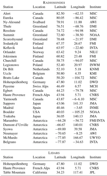
Table 1. List of GAW and NDACC ground-based stations used in this study.

RADIOSONDES

Station Location Latitude Longitude Institute

Alert Canada 82.50 −62.33 MSC

Eureka Canada 80.05 −86.42 MSC

Ny-Alesund Svalbard 78.91 11.88 AWI Thule Greenland 76.51 −68.76 DMI Resolute Canada 74.72 −94.98 MSC Summit Greenland 72.60 −38.50 NOAA Scoresbysund Greenland 70.48 −21.97 DMI Sodankyl¨a Finland 67.37 26.67 FMI Keflavik Iceland 63.97 −22.60 INTA

Orlandet Norway 63.42 9.24 NILU

Jokioinen Finland 60.82 23.48 FMI Churchill Canada 58.75 −94.07 MSC Legionowo Poland 52.40 20.97 INWM De Bilt Netherlands 52.10 5.18 KNMI

Uccle Belgium 50.80 4.35 KMI

Bratts Lake Canada 50.20 −104.72 MSC Hohenpeißenberg Germany 47.80 11.02 DWD Payerne Swiss Alps 46.49 6.57 MCH

Egbert Canada 44.23 −79.78 MSC

Haute Provence French Alps 43.94 5.71 CNRS Yarmouth Canada 43.87 −6–6.10 MSC

Sapporo Japan 43.06 141.33 JMA

Madrid Spain 40.46 −3.65 INME

Boulder USA 40.03 −105.25 NOAA

Tsukuba Japan 36.05 140.13 JMA

Marambio Antarctica −64.28 −56.72 FMI/INTA Dumont d’Urville Antarctica –66.67 140.01 CNRS Syowa Antarctica −69.00 39.58 JMA Neumayer Antarctica −70.65 −8.25 AWI McMurdo Antarctica −77.85 166.67 UWYO Belgrano Antarctica −77.87 −34.63 INTA

LIDARS

Station Location Latitude Longitude Institute Hohenpeißenberg Germany 47.80 11.02 DWD Haute Provence French Alps 43.94 5.71 CNRS Table Mountain California 34.23 117.41 JPL

are designed to work optimally in the –90◦C to 60◦C range, with a typical accuracy of 0.5 K (Antikainen et al., 2002; da Silveira et al., 2003; Nash et al., 2006). As described earlier in this section, Rayleigh lidar systems provide the vertical profiles of temperature between 30 and 70 km during night using the Rayleigh-scattering technique. The standard output of the lidar systems is a mean temperature profile per night, with a vertical resolution of 3 km, integrated over non-cloudy times. The Rayleigh lidar systems reach an accuracy of 1 K in the 35–65 km altitude range. We have selected available correlative data that offer a sufficient coincidence with ACE-FTS measurements using 31 sonde stations and 3 temperature lidars (Table 1). These stations form a robust set of independent correlative measurements of well-known quality (Keckhut et al., 2004). The coincidences are essentially located at high and middle latitudes where the majority of the ACE measurements occur.

3 Comparisons with ACE-FTS temperatures

Validation of a satellite sensor is an exercise in compromise, particularly for an occultation instrument with limited geo-graphical sampling (as is the situation here). It is virtually impossible for an ACE-FTS measurement and the validating measurement to be in the same place at the same time. As in all validation studies, we tried to achieve a balance be-tween spatial-temporal proximity and ensuring an adequate sample size to provide decent statistics (and to reduce the ef-fects of geophysical variability on the comparisons). The co-incidence criteria used in generating the comparisons varied from instrument to instrument, as described below. These criteria were selected in each case to make best use of the overlap between data sets.

When considering the proximity of measurements for vali-dation studies, a short discussion of horizontal resolution and measurement location is needed to elucidate the underlying assumptions implied by the word “coincidence” as used in this study. The horizontal resolution of a measurement varies greatly between the instruments used herein. As mentioned in Sect. 1, a satellite measurement using a limb-viewing ge-ometry (such as an ACE-FTS occultation measurement) has a path length of approximately 500 km through the atmo-sphere and thus each profile point is an average over this hor-izontal distance. In contrast, lidar measurements or in situ balloon measurements (such as radiosondes or SPIRALE) have much greater horizontal resolution and therefore are much more sensitive to local atmospheric structures. To find coincident measurements for comparisons, a location has to be assigned to each observation. For lidar observations, the measurement occurs at the location of the instrument. Ra-diosondes typically travel no more than 50–100 km from the launch site so for these comparisons the location of the mea-surement has been taken to be the same as the launch site. The coincidence criteria are more challenging for satellite observations (such as those made by ACE-FTS) because the satellite is moving along its orbit while it is making a mea-surement and thus, the profile meamea-surement does not occur over a single point on Earth. The ground track can cover sev-eral hundred km, so the location of a representative altitude has been used to identify the location of each occultation. For these comparisons, the latitude, longitude and time of the 30 km tangent point (calculated geometrically) was used as the location of the ACE-FTS occultation.

3.1 SABER

To compare ACE-FTS and TIMED/SABER temperature pro-files, the following coincidence criteria are adopted: 200 km or less in distance and 3 h or less in time. Data from 1 March 2004–31 August 2006 are used in these comparisons. As shown by Petelina et al. (2005), such tight coincidence criteria are necessary, particularly at mesospheric altitudes, where the spatial and temporal variability in the atmospheric

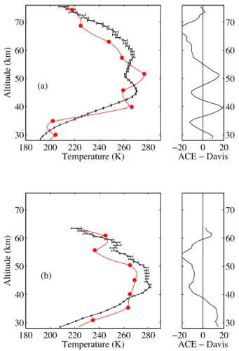
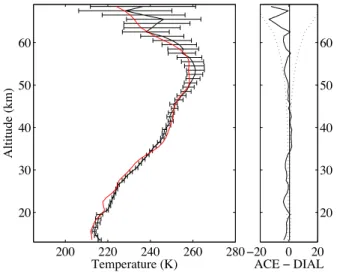
temperature field is significant (Sica et al., 2002). Examples of individual coincident ACE-FTS and SABER temperature profiles are shown in Fig. 1. As data from these two instru-ments are provided on different altitude grids, SABER pro-files have been interpolated onto the ACE-FTS 1-km grid us-ing cubic splines. Note that while individual profiles in Fig. 1 are shown for altitudes 11.5–100.5 km, the statistical analy-sis, as mentioned earlier, is restricted to the 11.5–70.5 km range where SABER temperature retrievals agree well with other data sets.

Fig. 1 (11 May 2005) shows that below 70 km good agree-ment between the instruagree-ments, within 2–5 K is found. Fig. 1 also shows an example on 14 August 2005 where the ACE-FTS version 2.2 profile (in red) exhibits unphysical oscil-lations in the mesosphere and thermosphere. Note that the high-frequency fluctuations in the residual profile (ACE-SABER) arise from these unphysical oscillations, while the broader structure in the residual profile is a consequence of geophysical differences between the two measurements. The cause of unphysical oscillations in ACE-FTS version 2.2 temperature profiles (along with the improvements im-plemented in the next generation ACE-FTS processing ver-sion) will be discussed in Sect. 4.

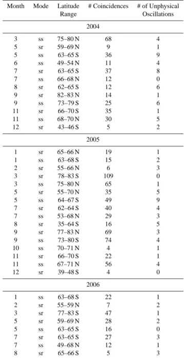
A summary of the monthly number of ACE-FTS and SABER coincidences and corresponding latitude ranges is given in Table 2 for the time period March 2004 through Au-gust 2006. The last column of the table shows the number of occultations in the group that were judged to contain unphys-ical oscillations. Problem occulations tend to occur in clus-ters, a consequence of the slow change in measurement con-ditions from occultation to occultation. It is therefore worth noting that for months with 20 or more coincidences, profiles with oscillations represent less than 25% of the total. Glob-ally, the number of occultations in this data set (for all years and all months) containing unphysical oscillations represents about 10% of the total.

In a preliminary version of the next generation ACE-FTS processing (to be called version 3.0), the unphysical oscilla-tions observed in the version 2.2 data set are removed. In a few cases, real structure in the mesosphere (judging from the SABER results) is suppressed in the preliminary version 3.0 results, a consequence of marginal sampling of the structure with the ACE-FTS measurements.

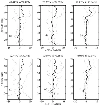
Mean differences and standard deviations for coincident ACE-FTS and SABER measurements are shown in Fig. 2 for a selected set of months. When considering all compar-isons below 45 km, the ACE-FTS and SABER data agree to within 1–2 K most of the time. The standard deviation range at these altitudes is also smallest. In March 2004, May 2005, and May 2006, differences between the two instruments be-low 15 km reached 3–4 K with ACE-FTS being larger than SABER. A number of the plots in Fig. 2 exhibit a “bump” in the comparisons near 23 km, with the ACE-FTS temper-atures about 2 K lower than the SABER tempertemper-atures. For altitudes above about 50 km, there is a systematic 2–3 K high

Table 2. Latitude range and number of coincidences with SABER for ACE-FTS sunset (ss) and sunrise (sr) occultations including number of occultations exhibiting unphysical oscillations in the mesosphere and thermosphere.

Month Mode Latitude # Coincidences # of Unphysical Range Oscillations 2004 3 ss 75–80 N 68 4 5 sr 59–69 N 9 1 5 ss 63–65 S 36 9 6 ss 49–54 N 11 4 7 sr 63–65 S 37 8 7 ss 66–68 N 12 0 8 sr 62–65 S 12 6 9 sr 82–83 N 14 1 9 ss 73–79 S 25 6 11 sr 66–70 S 35 1 11 ss 68–70 N 30 5 12 sr 43–46 S 5 2 2005 1 sr 65–66 N 19 1 1 ss 63–68 S 15 2 2 sr 55–66 N 6 3 3 sr 78–83 S 109 0 3 ss 75–80 N 65 1 5 sr 55–70 N 35 5 5 ss 64–67 S 49 9 7 sr 62–64 S 40 4 7 ss 53–68 N 29 3 8 sr 35–64 S 16 5 9 sr 77–83 N 69 3 9 ss 73–80 S 74 4 10 ss 70–71 N 4 1 11 sr 66–70 S 22 1 11 ss 67–71 N 56 4 12 sr 39–48 S 4 0 2006 1 ss 63–68 S 22 1 2 sr 55–59 N 7 2 3 sr 77–83 S 47 1 5 sr 59–69 N 28 2 5 ss 63–65 S 16 0 7 sr 63–65 S 27 3 7 ss 49–68 N 12 1 8 sr 65–66 S 5 3

bias of the ACE-FTS temperatures relative to SABER. This effect does not seem to have any seasonal or latitudinal de-pendence.

In a companion paper in this issue, individual comparisons of ACE-FTS and SABER temperatures are given by Man-ney et al. (2007), who show comparisons of individual ACE-FTS and SABER coincident profile pairs, as well as daily-averaged ACE-FTS, coincident MLS and SABER profiles.

150 200 250 20 40 60 80 100 Temperature (K) A lt it ude (km ) !20 0 20 20 40 60 80 100 ACE ! SABER 150 200 250 20 40 60 80 100 Temperature (K) A lt it ude (km ) !20 0 20 20 40 60 80 100 ACE ! SABER (a) (b)

Fig. 1. Typical examples of individual temperature profiles (left panels) for SABER v1.06 (black curve) and ACE-FTS v2.2 (red curve) and temperature differences (in K – right panels). As noted in the text, the oscillations in the ACE temperatures are not geo-physical variations. (a) ACE-FTS occultation on 11 May 2005 at 01:40:59 UT (66.29◦S, 163.41◦W) compared to SABER at 01:49:23 UT (65.78◦S, 160.48◦W). (b) ACE occultation on 14 Au-gust 2005 at 15:44:16 (42.22◦S, 21.80◦E) compared to SABER at 18:20:45 UT (42.36◦S, 22.39◦E).

3.2 MIPAS

MIPAS v4.62 temperature data are compared with ACE-FTS version 2.2 data for the period from 21 February 2004 to 26 March 2004. During the first five months of the ACE mission only sunsets were measured because of issues with spacecraft pointing at sunrise. Therefore the latitude coverage available for this comparison is limited to 20◦N to 90◦N.

Further limiting the comparisons of profile locations to 6 h time difference and 300 km horizontal difference produces regular matches in the 80◦N to 90◦N latitude region. The slightly relaxed temporal criterion has been chosen in order to increase the statistics of the comparison, which includes 137 coincident pairs. For each of the selected pairs, the MI-PAS temperature profiles were interpolated on the pressure

!!" " !" #" $" %" &" '" (" ) *+ ,+ -./ 0123 4 '(5%%°60+70("5%(°6 !!" " !" #" $" %" &" '" (" )890!0:);9< (&5#&°60+70(=5&'°6 !!" " !" #" $" %" &" '" (" ((5%!°60+70>$5$%°6 1a4 1b4 1c4 !!" " !" #" $" %" &" '" (" ) *+ ,+ -./ 0123 4 '#5%%°60+70'$58%°6 !!" " !" #" $" %" &" '" (" )9:0!06);:< ($5"(°60+70(85!'°6 !!" " !" #" $" %" &" '" (" (=5""°60+70=$5"(°6 1d4 1e4 1f4

Fig. 2. Mean temperature differences (in K) between coincident ACE-FTS v2.2 and SABER v1.06 temperature profiles for sunset (ss) and sunrise (sr) occultations (thick black lines) for selected cases in the Northern (top panels) and Southern (bottom panels) Hemispheres. Thin dashed lines indicate the standard deviations of the differences (a) November 2005 (56 ss coincidences), (b) March 2004 (56 ss coincidences), (c) September 2005 (69 sr coincidences), (d) July 2005 (40 sr coincidences), (e) September 2004 (25 ss co-incidences), and (f) March 2005 (109 sr coincidences). Related pa-rameters, such as the ACE-FTS sunset/sunrise occultation, latitude range, and number of coincidences, are given in Table 2.

grid corresponding to the 1 km altitude grid of the ACE-FTS data. This was done to enable a statistical analysis of col-located measurements having different vertical spacing. The interpolated profiles are used to calculate the differences in temperature values retrieved by ACE-FTS and by MIPAS.

Figure 3 shows the mean temperature profiles and differ-ences for MIPAS v4.62 (black) and ACE-FTS v2.2 (red) for the latitude region 80◦_{N to 90}◦_{N. MIPAS includes only}

day-time profiles. Differences between the two instruments are within 2–4 K at all altitudes. There is a small negative bias of the ACE-FTS temperatures relative to the MIPAS temper-atures below about 45 km, and there is a small positive bias above 45 km.

3.3 HALOE

The coincidence criteria used for the HALOE instrument were 500 km in horizontal distance and 4 h in time. These criteria provide a total of 53 coincidences: 33 in July 2004 in the latitude range 64–68◦N, five in September 2004 near

200 220 240 260 10 20 30 40 50 60 70 Temperature (K) A lt it ude (km ) !5 0 510 20 30 40 50 60 70 ACE ! <I>A? Latitude 80°N!C0°N

Fig. 3. Mean temperature profiles from MIPAS v4.62 (black) and ACE-FTS v2.2 (red) for the latitude region 80◦N to 90◦N (left panel) and temperature difference (in K – shown in right panel). Er-ror bars indicate the standard deviation of the mean of the MIPAS temperatures.

latitude 60◦N, 12 in January 2005 in the latitude range 63 to 68◦S, and three coincidences in August 2005 near 50◦S. A few coincidences from January and February 2004 were ex-cluded from the comparisons because of quality issues with ACE measurements early in the mission. HALOE measure-ments were interpolated onto the ACE-FTS standard 1-km grid using a cubic spline.

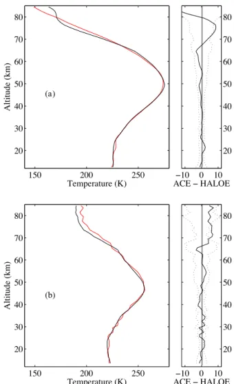
The results of the comparison between HALOE and ACE-FTS temperatures are shown in Fig. 4. The top panel of the figure shows the average differences for all 53 coinci-dences. Below ∼70 km, the agreement is good, within 2–4 K. Above 70 km, the discrepancies grow quite large. As noted in McHugh et al. (2005), the HALOE temperature retrieval suffers in accuracy in this altitude region in the presence of polar mesospheric clouds (PMCs). The majority of the coin-cidences between the two instruments occur in a location and season where one expects PMC formation. Only eight of the coincidences are not at risk of PMC effects in the HALOE temperature retrievals: the five coincidences in September 2004, and the three coincidences in August 2005. The lower portion of the figure shows the comparison using only these eight coincidences. With fewer measurements to average out geophysical variability, the portion of the curve below 70 km is somewhat noisier but still within 2–4 K. The differences above 70 km are dramatically improved compared to the re-sults for the full data set, consistent with the assumption of PMC contamination in HALOE temperature retrievals. In the comparison with the reduced data set, the ACE-FTS tem-peratures show a systematic hot bias of 5–6 K above 70 km.

!"# $## $"# $# %# &# "# '# (# )# *+,-+./01.+2345 6 70 80 19+ 23:, 5 !!# # !# $# %# &# "# '# (# )# 6;<2!2=6>?< 3a5 !"# $## $"# $# %# &# "# '# (# )# *+,-+./01.+2345 6 70 80 19+ 23:, 5 !!# # !# $# %# &# "# '# (# )# 6;<2!2=6>?< 3b5

Fig. 4. Mean temperature profiles (left panels) for HALOE v19 (black) and ACE-FTS v2.2 (red) and temperature differences (in K, right panels in solid black lines) with standard deviation of the differences (dotted black lines). (a) Results for all 53 coincidences, measurements within 500 km and 4 h. (b) Results from the subset of eight coincidences without the risk of PMC contamination on the HALOE temperature retrievals.

3.4 Davis, Antarctica Rayleigh-scatter lidar

In determining which ACE-FTS events to compare with, the following criteria were used. Only lidar data collected with the new telescope system were used for the Davis Lidar, which restricted comparisons to after late February 2005. ACE-FTS measurements must be within a 600 km radius of Davis and available within 6 h of the start or end of a li-dar observing session. These restrictions decreased the pos-sible comparison opportunities to 11. This number only marginally changed if the time or range restrictions were eased (e.g., to 1000 km radius or 12 h in time). The small

180 200 220 240 260 280 30 40 50 60 70 Temperat1re 3K5 A lt it 1de 3km 5 !20 0 20 30 40 50 60 70 ACE ! =avis 180 200 220 240 260 280 30 40 50 60 70 Temperat1re 3K5 A lt it 1de 3km 5 !20 0 20 30 40 50 60 70 ACE ! =avis 3a5 3b5

Fig. 5. Examples of the highly structured temperature field present in the Antarctic stratosphere. While both 28 July 2006 (a) and 30 July 2005 (b) show the same general features between the two in-struments, there are significant offsets in height. In the left panel, ACE-FTS v2.2 temperature profiles are shown by red lines (for the interpolated 1 km grid) and by solid red circles (for measurement grid results) and comparison instrument temperature profiles are shown by black lines. The error bars in the left panel are ±1σ standard deviation of the comparison instrument’s statistical error. In the right panel, temperature difference between the profiles is shown (in K).

number is a direct consequence of the geometry of the satel-lite measurements, which restricts the time of year when measurements are possible near Davis, and the fact that the lidar is only operated in fair weather conditions.

As an example of our comparisons, we consider the com-parison for ACE-FTS event sr15919 (Fig. 5). The ACE-FTS measurement was acquired approximately 500 km northeast of Davis at 03:40 UT on 28 July 2006. Lidar observations were conducted between 12:45 UT on 27 July and 01:19 UT on 28 July. The temperature field from the Atmospheric In-fraRed Sounder (AIRS) on the Aqua satellite at 1 hPa in the vicinity of Davis during the lidar measurements was used to

investigate spatial variations (Gettelman et al., 2004). Tem-perature variations of up to ∼15 K are apparent, with a gen-eral NW-SE gradient. The AIRS data show that horizon-tal temperature gradients of at least 5 K over a distance of 500 km can occur in the mid-stratosphere at this location. This scale of variability dominates over the measurement un-certainties for the 2 h resolution lidar retrievals at this al-titude. A second example of this variability is shown in Fig. 5 for 30 July 2005. Note the geophysical variability in each of these cases is greater than the statistical errors of the measurements, supporting our argument that large horizontal spatial temperature gradients exist.

During the winter and spring, Davis lies near the edge of the stratospheric polar vortex, and the vertical temperature profile, particularly in the stratosphere, can show relatively large meridional, zonal and vertical gradients due to dynam-ical effects related to the origin of the air (from inside or outside the vortex), planetary waves and gravity waves. In the summer, the stratosphere and mesosphere have generally less spatial and temporal variability compared to the winter. Comparisons with satellite temperature measurements from other instruments with closer spatial proximity to the Davis lidar show in general closer agreement than shown in Fig. 5 (Klekociuk et al., 2003).

3.5 Davis, Antarctica scanning spectrometer

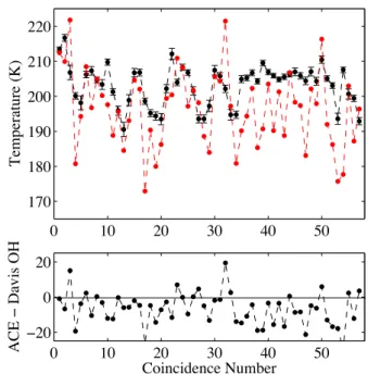
Nightly averaged OH(6-2) rotational temperatures in the mesopause region above Davis station, Antarctica have been compared with ACE-FTS v2.2 temperatures. Of the 94 avail-able occultations found within a 500 km radius of Davis, 57 had coincident nightly-averaged-hydroxyl-rotational temper-atures (Fig. 6). Nocturnal hydroxyl measurements are lim-ited to the period between mid-February and the end of Oc-tober at the latitude of Davis. The maximum nightly observ-ing time is about 19 h over mid-winter. Hydroxyl emissions typically originate in a layer centred near 87 km altitude and spanning about 8 km. In Fig. 6, hydroxyl temperatures are compared with the ACE-FTS 87.5 km grid point.

Of the 57 samples, the closest range separation is 126 km (average 361 km) and the nearest time difference from the OH nightly mean observing time is 4 hrs 40 min (average 9 h 10 min). Considerable atmospheric temperature vari-ability would be expected on these spatial and temporal scales. Nevertheless, for the 57 comparisons considered, OH temperatures were on average 5–7 K warmer than ACE-FTS measurements. The mean and standard deviation for the OH temperatures is 203.0±5.8 K compared to FTS v2.2 at 87.5 km, which is 196.3±10.9 K. If the ACE-FTS temperatures are weighted with a Gaussian centered on 87 km with a half width of 8 km using grid points from 73.5 km to 100.5 km, the mean and standard deviation be-comes 196.6±7.8 K, slightly closer to the OH-derived tem-peratures.

Using the Langhoff et al. (1986) transition probabilities increase the temperatures 2 K relative to other sets of tran-sition probabilities available. Given that the calibration un-certainty in these measurements is of the order of 0.3 K, the agreement between the Davis OH and ACE-FTS averages in-cluding both these factors is about 5 K. This result is reason-able considering the geophysical spatial and temporal vari-ability and the assumption of a typical (e.g. single humped) OH layer at 87 km altitude.

3.6 London, Canada lidar

Temperature retrievals from seven ACE-FTS measurements within 1000 km of the Purple Crow Lidar were compared with PCL temperature measurements for the entire night, both to compare any bias between the temperatures and to estimate retrieval error for ACE-FTS using the high tempo-ral resolution of the PCL. The PCL data was linearly interpo-lated onto the ACE-FTS measurement grid. Figure 7 shows examples of the agreement between the two instruments, highlighting the unphysical oscillations which can occur in the ACE-FTS v2.2 temperatures and the effect of a small-scale mesospheric inversion, which ACE-FTS can not re-solve. On 1 September 2005, the agreement between the two instruments is good, particularly in the lower mesosphere. However, above 70 km, the PCL measures a moderate tem-perature inversion, probably due to the interaction between tides and smaller-scale waves (e.g. Sica et al., 2002), which the ACE-FTS can not resolve. On 5 May 2006, the agree-ment is again good between the two instruagree-ments until above 65 km, where unphysical oscillations occur in the ACE-FTS measurements (see Sect. 4). The difference plots show the distance between the oscillations in the lower panel is on the order of the vertical spacing of the ACE-FTS measurements, characteristic of the unphysical oscillations, as opposed to the inversion structure observed in the top panel which is present over 5 ACE-FTS measurement points.

For the seven coincidences available, the ACE-FTS tem-peratures have a bias towards higher temtem-peratures than the PCL temperatures. The ACE-FTS temperature measure-ments are on average 5.5±1.8 K hotter than the PCL.

As mentioned previously, the ACE-FTS pres-sure/temperature retrieval routine is divided into two altitude regions. As described in Boone et al. (2005), there is a transition in the fundamental retrieval philosophy at the third measurement point above 43 km (typically between 50 to 60 km). We therefore consider separately the temperature bias in the two altitude regions. The low altitude region, taken as the altitude of the lowest PCL Rayleigh-scatter measurement (28 km) up to 60 km, shows no bias within the uncertainty (0.3±1.5 K). The high altitude region (taken as 60 to 95 km) has a bias of 5.9±2.1 K.

This calculation was repeated incorporating PCL Vibrational-Raman Scattering measurements (Argall et al., 2007). These measurements extend the comparison

down-0 10 20 30 40 50 170 180 190 200 210 220 T em pe ra ture (K ) 0 10 20 30 40 50 !20 0 20 A CE ! 9 a:i < = > C?i@Aide@Ae CumDer

Fig. 6. A comparison of 57 coincident Davis OH rotational tem-peratures (black) with ACE-FTS v2.2 temtem-peratures (red) at 87.5 km altitude (top) and differences (bottom; in K). The error bars on the OH rotational temperature time series are 1-σ standard deviation in the nightly mean.

wards to 12 km. Three additional coincident data sets also became available for this analysis (29 and 30 June 2005, and 5 May 2006). These results were comparable: an apparent bias of 5.4±2.0 K at high altitudes, and no detectable bias at low altitudes (0.4±1.6 K). In preliminary comparisons with results from the next generation of ACE-FTS processing software (the so-called “preliminary version 3.0”) with both the PCL Rayleigh Scattering and Vibrational-Raman Scattering results, there is no indication of a temperature bias (e.g. <0.5 K) in any altitude region.

At present, the ACE-FTS temperature retrieval algo-rithm does not generate error estimates from the pres-sure/temperature fitting procedure. This omission is due to the computational difficulties involved in propagating errors through the modified global fitting routine used in the ACE-FTS retrievals. Retrieval quantities are correlated. In the for-ward model calculation, errors in temperature can be com-pensated for through changes in associated pressure or tan-gent height, making it difficult to isolate a meaningful error estimate on a particular retrieval parameter.

To estimate the ACE-FTS contribution to the error, the geophysical and statistical errors as determined from the PCL measurements were calculated and subtracted in quadrature from the total variance as follows. The PCL statistical errors are determined by the photon counting statistics of the li-dar measurements (Measures, 1984). Geophysical variability

150 200 250 20 30 40 50 60 70 80 90 100 Temperature (K) A lt it ude (km ) !20 0 20 20 30 40 50 60 70 80 90 100 ACE ! PCL 150 200 250 20 30 40 50 60 70 80 90 100 Temperature (K) A lt it ude (km ) !20 0 20 20 30 40 50 60 70 80 90 100 ACE ! PCL

Fig. 7. Sample comparisons showing generally good agreement (in K) between the Purple Crow Lidar (black) and ACE-FTS v2.2 (red) temperatures on 1 September 2005 (top). In this case, ACE-FTS misses a small-scale mesospheric inversion. Comparison on 5 May 2006 (bottom), with the unphysical oscillations in the ACE-FTS v2.2 temperatures clearly visible. The agreement between the in-struments is particularly good in the mesosphere up to 65 km on this night where no clear inversion is present.

was estimated by calculating the RMS variation in the PCL measurements spaced by 30 min intervals over the night’s ob-servations. The ACE-FTS statistical error (σFTS) can then be estimated from the total error as follows:

σFTS=

q

(TPCL− TFTS)2− σ_PCLstat2 − σgeo2 (1) In the comparisons with the PCL Rayleigh lidar measure-ments, the bias of 5.9 K calculated previously was subtracted from the high altitude ACE-FTS data. Calculating the ran-dom error using Eq. (1) on these modified ACE-FTS data, the value obtained (averaged over all altitudes and measure-ment dates) was ±2.1 K. Incorporating the PCL

Vibrational-!"# $## $"# !# $# %# &# "# '# (# )# *# !## +,-.,/012/,3456 7 81 91 2:, 34;-6 !$# # $#!# $# %# &# "# '# (# )# *# !## 7<=3!3>7?3@9:0/ 4a6 !"# $## $"# !# $# %# &# "# '# (# )# *# !## +,-.,/012/,3456 7 81 91 2:, 34;-6 !$# # $#!# $# %# &# "# '# (# )# *# !## 7<=3!3>7?3@9:0/ 4b6

Fig. 8. Comparison of temperature profiles from K¨uhlungsborn li-dar (black) and ACE-FTS v2.2 (red) on 21 July 2005 (a) and on 24 July 2006 (b). The top comparison shows larger differences (in K) in the mesosphere, including an inversion layer measured by the lidar around 78 km.

Raman Scattering measurements in the analysis yields an es-timate of ±1.7 K for the lower bound of the ACE-FTS ran-dom error.

3.7 K¨uhlungsborn, Germany lidar

Comparisons between the lidar temperature profiles from K¨uhlungsborn and ACE-FTS soundings were performed for all soundings that are within a distance of 500 km and a time of 2 h. There were seven coincidences between Febru-ary 2004 and December 2006. The typical time difference between the compared profiles is about 1.5 h as the lidar soundings are only performed during darkness and the ACE-FTS observations during sunrise and sunset. The lidar tem-perature profiles were acquired over a 1 h integration time.

Within the limits of the measurements there is a general agreement between the different instruments from the mid-stratosphere up to the stratopause and no obvious bias of one of the instruments. Some wavelike structures in the tempera-ture difference profile between the two instruments (e.g. the lower plot in Fig. 8) appear to originate from the ACE-FTS data.

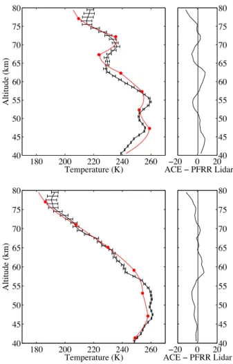
Above the stratopause, gravity and tidal waves become in-creasingly important, as is visible in the lidar measurements integrated for 60 min. Within the ACE-FTS profiles, most of this variation is not captured as a consequence of the vertical sampling (about 6 km in this case) for these ACE-FTS occul-tations coincident with the lidar. Apart from what appears to be an example of previously-mentioned unphysical oscil-lations in the ACE-FTS profile (likely induced by an under-sampled structure in the temperature profile), there is a good agreement between the ACE-FTS profile sr15870 on July 24 2006 (19:18 UT) and the lidar profile of 21:00–22:00 UT of the same day (Fig. 8). The spatial shift is only about 95 km, i.e., the profile is one of the nearest ACE-FTS measurements to the lidar station. The remaining difference between lidar and the ACE-FTS v2.2 temperatures above 60 km can be at-tributed to the different vertical resolutions. Given the vari-ability in mesospheric temperature structure observed with the lidar, one cannot expect excellent agreement in this re-gion for measurements collected at different times and loca-tions (Gerding et al., 2007b). However, accounting for this variability there appears to be a systematic high bias in the ACE-FTS temperatures above the stratopause. For most of the seven coincidences, ACE-FTS temperatures are about 1– 10 K higher than the lidar values below 80 km. Above 80 km, the differences increase. While one might expect the differ-ences in sampling to produce both positive and negative dif-ferences between the profiles, nearly all ACE-FTS profiles have higher temperatures than the lidar measurements. 3.8 Poker Flat Research Range, Alaska lidar

Comparisons between the lidar temperature profiles at Poker Flat Research Range and ACE-FTS measurements are per-formed for all ACE-FTS occultations within 100 km and 24 h of the lidar measurements. There are 10 such coincidences during six lidar observation periods between March 2004 and September 2005. The time difference between the compared profiles is as short as 1 h and as long as 24 h, with a typical value of 7 h as the lidar soundings are only performed during darkness and the ACE-FTS observations during sunrise and sunset. The lidar observations are integrated between 3 and 14 h, with an average of 9 h.

There is no obvious systematic bias between the satellite and lidar measurements. The differences between the mea-surements have similar magnitude in both the stratosphere and the mesosphere. These differences are both positive and negative below 75 km. There is a general positive bias in the lidar temperatures near 80 km that reflects a difference

between the ACE-FTS measurements and MSISE-90 model, which is used to seed the lidar temperature retrieval and can influence the retrievals in the upper mesosphere.

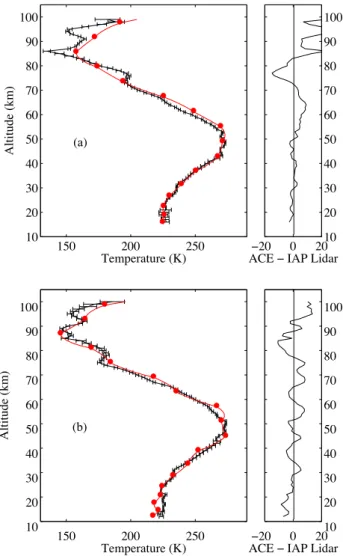
Two coincident measurements are shown in Fig. 9. There is no systematic bias between the ACE-FTS profile on Jan-uary 28 2005 (sr7881 at 14:08 UT) and the lidar profile ob-tained from 04:45–17:46 UT of the same day (top panel). The spatial difference between these measurements is less than 200 km. Despite the difference in the vertical resolu-tion of the measurements, both profiles show the same gen-eral features. Both the satellite and lidar measure a dou-ble maximum at the stratopause and a single maximum near 70 km. The maximum near 70 km appears to be a meso-spheric inversion layer with near adiabatic lapse rate be-tween 70 and 75 km. The ACE-FTS profile of 9 September 2005 at 16:12 UT (sr11181) and the lidar profile obtained between 06:08–09:15 UT of the same day show better agree-ment in the mesosphere than the stratosphere (Fig. 9 lower panel). The spatial difference for this coincidence is less than 500 km. The ACE-FTS temperatures are up to 5 K colder in the stratosphere, while the lidar temperatures are up to 5 K colder in the mesosphere.

3.9 SPIRALE flight from Kiruna, Sweden

One SPIRALE flight was successfully completed near Kiruna (Sweden, 67.7◦N, 21.6◦E) on 20 January 2006. A vertical profile of temperature was measured during the slow balloon ascent, between 17:50 and 19:50 UT. Pressure and temperature measurements were acquired every 1.1 s, pro-viding a vertical resolution of about 1 to 4 m. However this resolution has been degraded to 1 km by averaging all SPI-RALE results within each 1 km layer for comparison with ACE-FTS data. The best coincidence has been obtained for the ACE-FTS occultation sr13151, which occurred 12–13 h later (21 January 2006, 08:00 UT) at a distance of about 400 km (64.3◦N, 21.6◦E) from the SPIRALE balloon mea-surement. Therefore, prior to the intercomparison, the SPI-RALE profile was corrected for this spatial and temporal mismatch. The correction was done according to Eq. (C15) of von Clarmann (2006) and using temperature profiles ob-tained by interpolating in space and time ECMWF fields with a spatial resolution of 0.5◦×0.5◦and a temporal resolution of 3 h. The intercomparison of SPIRALE and ACE-FTS mea-surements is shown in Fig. 10. The altitude range selected for temperature comparisons is from 14 to 27.4 km, where data are available for both instruments. The SPIRALE in situ pro-file does not show any vertical oscillation features, unlike the ACE-FTS profile, which gives a second temperature mini-mum around 23 km height similar to SABER. This feature is likely an artifact in the retrieval due to the empirical form of the pressure profile employed (Sect. 4). In a comparison with a preliminary version of the next generation ACE-FTS temperature retrievals (e.g. v3.0), the feature is no longer evi-dent. The ACE-FTS temperatures are on average about 3.2 K