Observing Regularities in Location Patterns : An Analysis of the Spatial Distribution of Economic Activity in Spain

(1)

2005-08 OBSERVING REGULARITIES IN LOCATION PATTERNS. AN ANALYSIS OF THE SPATIAL DISTRIBUTION OF ECONOMIC ACTIVITY IN SPAIN Mario POLÈSE Fernando RUBIERA-MOROLLÓN Richard SHEARMUR

INRS

Urbanisation, Culture et Société

OCTOBRE 2005

(2)

(3)

Mario POLÈSE

Fernando RUBIERA-MOROLLÓN Richard SHEARMUR

Observing Regularities in Location Patterns :

An Analysis of the Spatial Distribution of

Economic Activity in Spain

Institut national de la recherche scientifique Urbanisation, Culture et Société

(4)

Mario Polèse

[email protected]

Université du Québec, INRS Urbanisation, Culture et Société, Montréal. Canada

Fernando Rubiera-Morollón

[email protected]

Universidad de Oviedo. Oviedo. España

Richard Shearmur

[email protected]

Université du Québec, INRS Urbanisation, Culture et Société, Montréal. Canada

Inédits, collection dirigée par Richard Sheamur Institut national de la recherche scientifique Urbanisation, Culture et Société

3465, rue Durocher

Montréal (Québec) H2X 2C6 Téléphone : (514) 499-4000 Télécopieur : (514) 499-4065 www.inrs-ucs.uquebec.ca

(5)

List of table and figures

Table 1 - Summary Data on the Eight Largest Metropolitan and Urban Areas in Spain (2003) .. 6

Figure 1 - Schematic Representation of the Classification of Spatial Units ... 5

Figure 2 - Spanish Cities Ranked According to Population (1996) ... 8

Figure 3 - A Schematic Map of the SR1 and SR2 Metropolitan Areas and Their Respective Central Areas of Influence... 10

Figure 4 - Ideal Model: Hieratical Distribution ... 13

Figure 5 - Ideal Model: Contained Deconcentration... 14

Figure 6 - Ideal Model: Unbounded Deconcentration ... 15

Figure 7 - Agriculture, Hunting and Forestry Activities and Fishing ... 17

Figure 8 - Construction... 19

Figure 9 - Manufacturing ... 20

Figure 10 - Wholesale and Retail Trade, Repair of Vehicles and Household Goods ... 22

Figure 11 - Hotels and Restaurants ... 22

Figure 12 - Financial Intermediation... 24

Figure 13 - Real Estate, Rental and Business Services ... 25

(7)

Summary

This study examines the location of economic activity in Spain for the years 1991 and 2001, employing a framework previously applied to Canada, which emphasizes the role of distance and urban size. Using census data, Spain’s 8,086 municipalities are classified according to their population size and distance from major metropolitan areas. The location of industry is then plotted in relation to these classes. On the whole, results display regular spatial distributions consistent with classic location theory and previous findings. No major alterations in location patterns were observed over time, confirming the continued importance of distance and of agglomeration economies. However, the results reveal a vigorous crowding-out process, fuelling the growth of manufacturing activity in locations in close proximity to metropolitan areas.

(8)

(9)

Introduction

This paper is part of an on-going research effort to describe (and, hopefully, better explain) national industrial location patterns using a common framework. In this paper, the framework (henceforth called “the model”) is applied to the Spanish case, building on previous applications in Mexico and Canada (Polèse and Champagne 1999 and Polèse and Shearmur 2004). The basic premise of the model is that the location of most economic activity can be understood in terms of two simple variables, distance and size. By the same token, we posit that the spatial distribution of comparable industries will display analogous patterns in different nations, barring dramatic differences in geography and history. The methodological challenge is one of suitably defining the distance and size variables for each country studied. We suggest here that the appropriate size and distance thresholds (especially the latter) may not vary all that much between nations, despite differences in nation size and geography. In this paper, the same thresholds (with minor variations) are applied to Spain as those used for Canada in previous studies.

The empirical focus of this paper is on Spain. Thus, a large part of the study is devoted to the description of results for that nation. Nonetheless, our ultimate aim remains a better understanding of industrial location patterns in general. Following a brief review of the relevant literature on industrial location, we present the building blocks of the model, together with a summary of earlier findings for Canada; it is not assumed that the reader is familiar with previous work. We ask why results for Spain should differ, and then proceed to present our results.

(10)

1. ON THE ROLE OF DISTANCE AND SIZE IN EXPLAINING LOCATION PATTERNS

Many, if not most, location decisions may be viewed in terms of a trade-off between

agglomeration economies and diseconomies, in other words choices between larger and

smaller cities. Classic Christallerian central place theory implicitly postulates a hierarchical distribution of services based on city size, depending on the production and consumption characteristics of the service in question, notably its sensitivity to distance. For manufacturing, Henderson (1997) has elegantly explained the trade-off between the costs and benefits of locating in cities of various sizes. The premise that cities, or rather urban regions, constitute distinct land and labour markets, an attribute founded on distance, is central to Henderson’s argument. Indeed, size only matters because the “cities” or other locations (postulated by any location model) are spatially separated, that is, distant from one another. Were this not so, it would make little sense to speak of a trade-off between agglomeration economies and diseconomies.

In less abstract terms, the advantages derived from large-scale production and the positive externalities associated with size lead to the concentration of economic activity in central locations with access to the largest possible market. Transportation costs curb this concentration behaviour, but the extent of this limitation depends on the activity’s consumption characteristics. Those activities that require intense personal interaction between consumers and producers (many services) and/ or are consumed daily or very frequently will display quasi-equal distributions over space. In contrast, those activities that are tradable over broader distances, not requiring proximity to the point of consumption, and/ or are demanded less frequently will concentrate their production in a limited number of central locations. As distance costs fall and trade increases, larger concentrations tend to expand. A shift in the national economy towards agglomeration sensitive goods and services (out of agriculture, for instance) also favours the growth of larger concentrations.

As large concentrations grow, diseconomies naturally appear, producing an expulsion effect for some activities. Wages and land prices are in part a function of city size. Wage-sensitive and space-extensive activities will be pushed out by what is sometimes called the “crowding-out effect” of rising wages and land prices in large metropolitan areas (Ingram 1998, Graham and Spence 1997). This crowding-out effect will most notably be felt by

(11)

medium-technology manufacturing, which has less need of the highly skilled labour in large cities (Henderson 1997), but also by wholesaling and distribution, extensive consumers of space, giving rise in turn to the growth of smaller cities.

On the other hand, on the side of agglomeration economies, when an urban concentration is created, firms within the same industry benefit through lower recruitment and training costs (shared labour-force), knowledge spillovers, lower industry-specific information costs and increased competition (Rosenthal and Strange 2001, Beardsell and Henderson 1999, Porter 1990). The increasing size of the metropolis makes certain infrastructures, such as international airports, post-graduate universities and research hospitals, possible. Recent literature stresses the positive link between productivity and the presence of a diversified, highly qualified and versatile labour pool (Duraton and Puga 2002, Glaeser 1998, 1994, and Quigely 1998). As underlined by Hall (2000) and Castells (1996), large metropolises stimulate the exchange of knowledge.1 Activities characterized by the need for high creativity and innovation will generally choose to locate in major metropolitan areas or nearby, a point to which we shall return.

It is reasonable to infer that the trade-off between the positive and negative effects pushing economic activities towards large cities or, alternatively, driving them out, should give rise to an economic landscape characterized, ideally, by regularities in industrial location patterns based on city size and on distance from other (smaller) cities. This inference provides the conceptual foundation for our model (see next section).

However, before presenting the model, we need to briefly address the possible impact of information technology (IT) on distance. Some, most notably Cairncross (2001), have heralded the death of distance. We found no evidence of a reduced distance effect in our previous work (Polèse and Shearmur 2004). In this we are not alone. Gasper and Glaeser (1998) suggest that new IT is not a substitute for face-to-face contacts; on the contrary, it is often complementary, fuelling the need for more business meetings, and increasing the demand for agglomeration economies. Along the same lines, Kotkin (2001) predicts an increase in the relevance of proximity for knowledge-based economies. Others also have suggested that the anticipated revolutionary impacts of recent technological change are

(12)

probably much exaggerated (Ghemawat 2001, Gordon 2000). In our study of Spain, it will be instructive to see how the distance variable behaves over time.

Schematic Presentation of the Model

The model used here is part of the family of models developed by Coffey and Polèse (1988), Polèse and Champagne (1999) and Polèse and Shearmur (2004). In practical terms, the model entails the classification of spatial statistical units (census divisions, metropolitan statistical areas, regions, etc.) that comprise the national space economy by population size and distance (from the largest metropolitan areas). The resulting new spatial observations, named Synthetic Regions (SRs), are groupings of analogous statistical units, classified by size and distance. For studies over time, geographies must be standardized.

Figure 1 presents a schematic representation of a model national space economy. The reader will undoubtedly note the resemblance to the classic economic landscape models of Christaller, Lösch, and Von Thünen, all of which posit one central metropolis or marketplace. Thus, Figure 1 posits one metropolis at the centre, but also four classes of smaller “central” urban areas of various population sizes (urban areas close to the metropolis) as well as “central” rural areas (close to the metropolis). Four analogous size classes are posited for “peripheral” urban areas, located at some distance from the metropolis, surrounded by corresponding rural localities. It is implicitly assumed that urban areas are distributed in accordance with the rank-size rule. Finally, three “ultra-peripheral” urban areas and corresponding rural areas are shown in Figure 1. This constitutes a departure from previously applied models, introduced because of Spain’s geography (more on this below).

As each country requires the definition of appropriate size and distance thresholds to translate this model economic landscape into operational statistical classes (SRs), we will now establish these parameters for Spain.

(13)

Figure 1. Schematic Representation of the Classification of Spatial Units Metropolitan area Central urban areas Central rural areas Peripheral rural areas Peripheral urban areas Ultra peripheral urban areas Ultra peripheral rural areas

Adapted from Polèse and Shearmur (2004).

2. DATABASE: REDEFINING OF SPANISH ECONOMIC SPACE

Database

The data employed is drawn from the Spanish Census, administered by INE (the National Statistics Institute of Spain). Although these are partially up-dated every three years, complete databases are only available every decade. The last two available Spanish censuses are for 1991 and 2001. The database comprises employment figures for sixteen (16) industrial classes; see Appendix B for more details of the activities included in each class.

As regards spatial units, Spain is divided into seventeen Autonomous Communities, some of which are composed of provinces, for a nationwide total of 52 provinces, each of which is in turn divided into municipalities, from 35 to 370. In 2001 there were some 8,086 municipalities in Spain.2 The Census provides population and employment data for each municipality. Metropolitan areas were defined in accordance with the guidelines of the

(14)

Ministerio de Fomento3 report on Spanish urban areas (MFON 2004), allowing us to identify the municipalities in each metropolitan area. Precise definitions of metropolitan areas can be found in Appendix A.

Table 1 presents summary data for the eight most important Spanish urban areas. These metropolitan areas account for more than one third of the total population of Spain and close to 40 per cent of its GDP. The areas of Madrid and Barcelona are of special relevance, as are the Ebro axis (Zaragoza) and the Cantabrian coastal strip (centred on the Bilbao metropolitan area). For a detailed analysis of the Spanish metropolitan system, see Roca and Burns et al. (2001) and MAP (2001).

Table 1. Summary Data on the Eight Largest Metropolitan and Urban Areas in Spain (2003)

Area Number of municipalities included Population (2003) Population density per km2 (2003) Percentage of the total Spanish population (2003)

Metropolitan area of Madrid 28 5,085,947 2,550.6 11.91

Metropolitan area of Barcelona 164 4,616,279 1,405.3 10.81

Metropolitan area of Valencia 44 1,426,442 2,244.3 3.34

Metropolitan area of Seville 25 1,211,041 723.4 2.84

Metropolitan Bilbao 35 903,866 1,679.8 2.12

Central area of Asturias 18 814,261 556.2 1.91

Malaga 7 789,930 1,077.7 1.85

Zaragoza 2 638,661 590.8 1.50

Source: MFON (2004).

Classification of Spanish Areas

In accordance with the information provided in the previous section, Spanish areas are defined as follows:

• Metropolitan areas (SR1 and SR2): metropolitan areas of more than five hundred

thousand inhabitants in 1996 (a median year in the decade under analysis, 1991-2001).

(15)

The 500,000 threshold is the same as that used in Polèse and Shearmur (2004) to define metropolitan areas for Canada. For Spain, metropolitan areas are sub-divided into two classes. The first, SR1, includes metropolitan areas with more than two and a half million inhabitants. The second, SR2, refers to metropolitan areas with a population of between 500,000 and 2,500,000 inhabitants. This is an empirical criterion based on observation of Spanish data. As can be seen in Figure 2, the 2 ½ million population line, between SR1 and SR2, is the point at which a clear distinction appears between Spanish cities. In the Canadian case, the one million mark was used to distinguish between SR1 and SR2.

• Urban areas (SR3, SR4, SR5 and SR6): urban agglomeration areas with more than ten

thousand inhabitants in 1996. These are grouped into four classes. The first, SR3, includes all areas with more than 100,000 inhabitants and less than 500,000; the second,

SR4, all urban areas with populations between 50,000 and 100,000 inhabitants; and the

third, SR5, all urban areas between 20,000 and 50,000 inhabitants. Finally, SR6 refers to urban areas with more than 10,000, but less than 20,000 inhabitants. Again, these classes are analogous to those used for Canada.4

• Rural areas (SR7): all areas that are not urban areas, which may contain towns, but with

less than ten thousand inhabitants in 1996.

(16)

Figure 2. Spanish Cities Ranked According to Population (1996) 0 500000 1000000 1500000 2000000 2500000 3000000 3500000 4000000 4500000 5000000 SR1 areas SR2 areas Source: MFON (2004).

A parallel distinction, based on proximity to major metropolitan areas, is applied to all non-metropolitan SRs:

• Central areas (SRC): all areas within approximately one hour’s drive of a

metropolitan area (SR1 or SR2). Account has been taken of road conditions (highway or not), the spatial limits of metropolitan areas, and the characteristics of the area being classified. Thus, central areas do not necessarily form perfect rings around metropolitan areas, as posited in the model landscape in Figure 1. The one-hour threshold, also used in Canadian applications, was found to be very robust, a good indicator of the range within which spatial interaction with the metropolis remains fairly easy, especially for face-to-face relationships related to the consumption of higher-order services.

• Peripheral areas (SRP): all areas situated farther than one hour’s drive from

(17)

• Ultra-peripheral areas (SRUP): islands and territories located outside the Iberian

Peninsula.

Figure 3 shows the location of SR1 and SR2 on the map of Spain, together with a schematic approximation of their central areas of influence, falling within the one-hour range. Madrid’s “area of influence” describes a circle that is fairly equidistant from the city of Madrid, embracing the entire Autonomous Community of Madrid and the cities of Toledo, Guadalajara, Avila and Segovia. Barcelona’s reach extends to the other two main cities on the northeastern coastal strip: Gerona to the north of Barcelona and Tarragona to the south. Barcelona’s area of influence is less circular than that of Madrid due to the nature of road links between the three aforementioned urban centres. Lleida, the fourth largest city in Catalonia, located inland, is not included in Barcelona’s area of influence because it falls beyond the one-hour threshold.

Valencia’s area of influence spreads northward along the coast to the city of Castellón and over all the Community of Valencia. To the south, it overlaps with Alicante’s area of influence; the latter also covers some of the Murcia-Cartagena area in the province of Murcia. This means that most of the Mediterranean coast is classified as central. In the south of Spain, Seville, Malaga and Cadiz Bay together form a sprawling central area of influence that embraces almost all three provinces, apart from the northern mountain range of Seville and the eastern part of the province of Huelva, located close to Seville. On the Cantabrian coast, Bilbao’s influence extends over the provinces of Vizcaya, Guipúzcua and Álava, i.e. all of the Basque Country, and the north of Burgos and east of Cantabria, including, in the latter case, the cities of Santander and Torrelavega. In contrast, the mountainous geography that characterizes the Asturias region, also on the northern coast, and its poor road links limit the extension of the Asturias urban conurbation’s influence beyond its boundaries.

(18)

Figure 3 - A Schematic Map of the SR1 and SR2 Metropolitan Areas and Their Respective

Central Areas of Influence

Madrid metropolitan area (R1) Barcelona metropolitan region (R1) Central urban area of Asturias Valencia metropolitan area (R2) Metropolitan area of Sevilla (R2) Málaga (R2) Cádiz Bay (R2) Bilbao metropolitan area (R2)

Alicante urban area (R2)

Murcia and Cartagena urban area (R2)

Zaragoza (R2)

Main cities Central area Ultra-peripheral area

Metropolitan area Peripheral area

Summarizing, we have the following Synthetic Regions for Spain:

SR1: metropolitan areas of more than 2,500,000 million inhabitants. SR2: metropolitan areas of between 500,001 and 2,500,000 inhabitants. SR3C: central urban areas of between 100,001 and 500,000 inhabitants. SR4C: central urban areas of between 50,001 and 100,000 inhabitants. SR5C: central urban areas of between 20,001 and 50,000 inhabitants. SR6C: central urban areas of between 10,001 and 20,000 inhabitants. SR7C: central rural areas, with less than 10,000 inhabitants.

SR3P: peripheral urban areas of between 100,001 and 500,000 inhabitants. SR4P: peripheral urban areas of between 50,001 and 100,000 inhabitants. SR5P: peripheral urban areas of between 20,001 and 50,000 inhabitants. SR6P: peripheral urban areas of between 10,001 and 20,000 inhabitants. SR7P: peripheral rural areas, with less than 10,000 inhabitants.

SR3UP: ultra-peripheral urban areas of between 100,001 and 500,000 inhabitants. SR4UP: ultra-peripheral urban areas of between 50,001 and 100,000 inhabitants. SR5UP: ultra-peripheral urban areas of between 20,001 and 50,000 inhabitants. SR6UP: ultra-peripheral urban areas of between 10,001 and 20,000 inhabitants. SR7UP: ultra-peripheral rural areas, with less than 10,000 inhabitants.

(19)

The rest of Spain, comprising the white areas on the map (Figure 3), is classified as

peripheral (both urban and rural). Clearly, the east and northeast of the country, as well as

the regions surrounding Madrid’s area of influence, with the exception of the Ebro axis, are the most extensive peripheral territories. These include the Autonomous Community of Galicia, incorporating several medium-sized cities (principally La Coruña and Vigo), as well as the Communities of Extremadura, Castilla y Leon, Castilla la Mancha, La Rioja, and the provinces of Huesca and Teruel (belonging to the Community of Aragon).

Finally, the Islands (Canaries and Balearics) and the cities of Ceuta and Melilla, in North Africa, are classified as ultra-peripheral areas.

388 municipalities (4.8% of the total number) are classified as SR1 and SR2, 706 municipalities (8.7%) as SR3, SR4, SR5 or SR6. The remaining 6,992 municipalities are classified as SR7, i.e. as rural areas. About 16% of non-metropolitan municipalities are classified as central areas. 152 municipalities are in ultra-peripheral areas. The remainder are peripheral.

The small number of ultra-peripheral observations and their geographical and economic specificities5 suggest limited generalizability. While overall results for SRUP will be provided, they should be interpreted with caution. In only some cases, specifically those related to tourism, will we consider SRUP results. Our focus is on the differences between central and peripheral locations. All data are by place of residence. This should be borne in mind when interpreting the results, since it is possible that jobs are located in areas other than the place of residence. This is of particular relevance for spatial units in the rural central class (SR7C) directly adjacent to metropolitan areas. This caveat does not invalidate our analysis, but can influence our interpretation of certain results.

Location quotients are calculated for sector employment for each SR. The analysis is not based upon mean values of location quotients but rather on location quotients calculated for each SR in its entirety. Thus,

5

Ceuta and Melilla only count as two municipalities. The remaining 150 municipalities belong to the Balearic and Canary Islands, whose economy is largely based on tourism.

(20)

E E e e LQ x n i a i n i a xi Xa ⎥ ⎦ ⎤ ⎢ ⎣ ⎡ ⎥ ⎦ ⎤ ⎢ ⎣ ⎡ =

∑

= = 1 1 where :

LQxa = location quotient of sector x in synthetic region a,

n = number of spatial units in synthetic region a,

eaxi = employment in sector x in spatial unit i in synthetic region a,

eai = total employment in spatial unit i in synthetic region a,

Ex = total employment in sector x in Spain, and

E = total employment in Spain.

Model Location Patterns and Expected Results

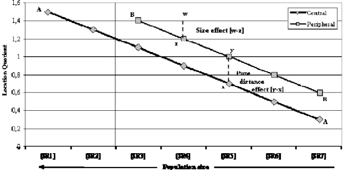
The results are best interpreted with graphic aids (see Figure 4 and subsequent figures). Based on Polèse and Shearmur (2004) and Polèse and Champagne (1999), we should expect to find certain stylised patterns, notwithstanding the specifics of the Spanish case. In Figures 4, 5 and 6, the vertical axis provides the relative concentration levels (location quotients) for the activities studied and the horizontal axis identifies the locations (SRs) in order of descending population size from left to right. Note that there are only seven (and not twelve) classes, because the values for central and metropolitan areas are given on one curve (A) and the peripheral values on another (B). A third curve (C) could possibly be plotted for ultra-peripheral areas, but, for the reasons stated above, we will focus our attention on the differences between central and peripheral areas.

Figure 4 presents a perfectly symmetrical and hierarchical distribution of economic activity as predicted by Christallerian central place theory and the effects of spatial competition for demand-oriented commodities. This behaviour would be expected for activities primarily sensitive to city size. Sensitivity to distance (specifically, distance from a metropolitan area) is measured by the gap between curves A and B. In the case of Figure 4, curve B

(21)

always lies above curve A, signifying that, for any given city size, values will be systematically higher for peripheral urban areas located at some distance from a metropolitan area. We call this the distance effect. Here, this also represents a

distance-protection effect, since peripheral locations have higher values than those nearby.

Polèse and Shearmur (2004) found in the Canadian case that activities such as financial, producer and professional services fit the pattern most closely. However, while the size

effect behaved as expected (downward sloping), the distance effect was found to be

negligible for these services, although in the right direction. A priori there is little reason to think that the results should differ greatly in the Spanish case. Studies on the location of higher-order services in Spain have generally noted a positive relationship with city-size (Gago 2000, Martínez and Rubiera 1999, Rubalcaba and Gago 2003, Rubiera 2005). Perhaps, we might expect an even weaker distance effect given the smaller distances in Spain than in Canada, that is, within peripheral space beyond the one-hour threshold.

Figure 4 - Ideal Model: Hieratical Distribution

Source: Polèse and Shearmur (2004).

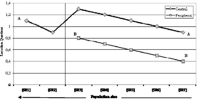
Figure 5 illustrates what we call contained deconcentration, in which, in contrast to the previous example (Figure 4), proximity to a metropolitan area is a positive factor.

(22)

Applications to Canada and Mexico have demonstrated that activities best approximated by this model are found in the manufacturing sector, especially medium value-added industries sensitive to land prices and labour costs and, as such, crowded-out of metropolitan areas. The distance effect is the primary determinant. Given the choice, most manufacturing firms will prefer to locate in medium-sized cities close to a major metropolitan area. Again, we should expect similar results for Spain. Various Spanish studies have noted the tendency of manufacturing to concentrate in medium-sized cities close to major metropolitan areas (Alonso, Chamorro and González 2004, Paluzie, Pons and Tirado 200, Trueba and Lozano 2001). However, here again, the combination of smaller distances (beyond central locations) and the more equidistant distribution of cities may affect the impact of the

distance effect, reducing its significance.

Figure 5 - Ideal Model: Contained Deconcentration

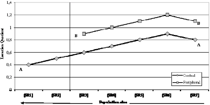
Finally, Figure 6 represents the opposite case, called unbounded deconcentration, in which activities react negatively both to city size and proximity (to a metropolitan area). Curve B is above A, indicating that cities far from metropolitan areas are preferred, while the

(23)

upward-moving slopes indicate that smaller cities are also favoured. This pattern would be expected to describe traditional Weberian weight loss activities tied to heavy primary inputs that are most cheaply available in remote (non-metropolitan) locations.

Consequently, this pattern should approximate that of resource-dependent activities and of low value-added, wage-sensitive industries, which do not need to be near a major metropolis. Yet here again, there is little reason to believe that the results for Spain differ substantially.

Figure 6 - Ideal Model: Unbounded Deconcentration

Descriptive statistics (Appendix C) supplement the figures:

• Size effect: the slope of the curve linking LQs of urban areas of a given type (central,

peripheral, and even ultra-peripheral) between classes SR3 and SR6, assuming unit distance between adjacent classes. Metropolitan areas (in central SRs) and rural areas are excluded. The results provided have been multiplied by 100. Since the largest urban areas are to the left of the figure, a positive result (i.e. positive relationship between city size and LQ) is associated with a downward sloping curve.

(24)

• Distance effect: the average difference between the value of LQs for central and

peripheral SRs in the same class, once again for that part of the curve falling between

SR3 and SR6. A positive value means that curve A (central) lies above B (peripheral).

• Metropolitan effect: the ratio of the highest SR1 or SR2 (metropolitan) LQ value to

the average highest value among urban SRs (from SR3 to SR6 classes).

• Primacy effect: the ratio of the LQ value of SR1 to SR2.

• Rural effect: the ratio of the average value of peripheral rural LQs to urban LQs.

• Central rural effect: the ratio of the LQ value of SR7C and SR7P.

• Ultra-peripheral specificities effect: the average difference between the value of LQs

for the average of central and peripheral and the ultra-peripheral SRs in the same class, once again for that part of the curve falling between SR3 and SR6.

• Main peripheral cities effect: the ratio of the SR3UP (main cities in the

ultra-peripheral areas) LQ value to the highest value among all other urban SRUPs (from

SR4UP to SR6UP).

• Ultra-peripheral rural effect: the ratio of the LQ value of SR7UP and SR7P.

3. RESULTS:LOCATION PATTERNS OF ECONOMIC ACTIVITY IN SPAIN 1991,2001

Results for the Spanish economy are presented in the following pages. We shall concentrate on analyzing the location patterns of manufacturing and service activities. A complementary objective is to examine shifts over time, although the period studied is relatively short (1991 - 2001). However, this is the decade in which information technologies (IT) experienced their most rapid rise and spatial diffusion in Spain (Soto, Pérez and Feijóo 2003). Although direct causality between observed shifts in location patterns and the effects of IT cannot be inferred from our results, we shall nonetheless (cautiously) attempt to draw some conclusions, specifically for those sectors a priori most affected by IT. Where appropriate, we shall relate our findings to those of earlier applications to Canada. For reasons of space, we present figures only for selected industrial classes. However, descriptive statistics for all industrial classes are given in Appendix C.

(25)

Primary and Secondary Employment

Figure 7 shows results for sectors A and B of the Spanish ISIC classification, covering the first two classes of the primary sector. As can be seen, the results approximate the idealized

unbounded deconcentration model (Figure 6). There is a clear upward slope in both curves,

and the central curve falls below its peripheral counterpart. In other words, these activities tend to locate in small cities and especially in rural areas, displaying a clear tendency to flee metropolitan areas of influence. The agriculture, hunting and forestry sector shows the largest rural effect statistic (see Appendix C), indicating that this is the activity most concentrated in rural areas, as one would indeed expect. The high value for SR4P on Figure 7 is largely attributable to medium-sized (peripheral) cities that are heavily specializedspecialized in fishing, most of which are located in the Autonomous Community of Galicia, on the northwest coast of Spain. No marked shifts in the location pattern are observable from 1991 to 2001. In sum, the results are predictable, consistent with the expected location patterns of primary activities.

Figure 7 - Agriculture, Hunting and Forestry Activities and Fishing

(26)

The mining and quarrying sector (figure not shown) also presents a close fit to the

unbounded deconcentration model, which again should come as no surprise since it largely

follows the location of natural resource deposits.6 On the whole, primary sector employment was found to follow very similar patterns in Canada (Polèse and Shearmur 2002).

The results for the secondary sector are more interesting, since less predetermined by geography. Unfortunately, the analysis is strongly limited by the classification employed by the Spanish census office. All manufacturing is treated as a single sector. However, before looking at manufacturing, let us briefly consider construction. As witnessed in Figure 8, the

distance effect barely exists for construction. Nonetheless, a clear upward slope can be

observed. These are space-consuming activities, not necessarily requiring highly skilled labour, with a tendency to be situated outside major metropolitan areas. The construction sector is disposed to locate in small-to-medium sized cities with no preference between central or peripheral areas. The absence of a distance effect suggests that this is largely a local (non-tradable) activity, consistent with what one would expect to observe, but one which tends to locate outside the larger urban areas serviced.

6

A strong concentration around the municipalities of Leon, Orense and Asturias can be observed. Leon belongs to the Autonomous Community of Castilla y Leon and is in the central northern part of the country. Orense is a Galician province and is located close to Leon (in the northwest). Asturias is a uni-provincial Autonomous Community located close to the other two provinces on the north coast. The area possesses important coal deposits, which historically have had a major impact on industrial structure.

(27)

Figure 8 - Construction

Source: Authors’ calculations based on INE (1991, 2001).

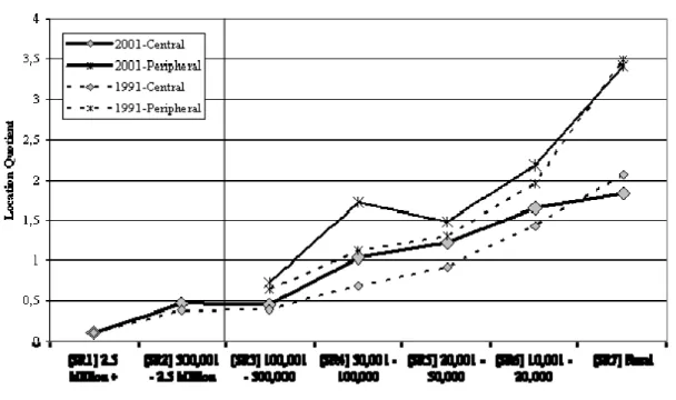
The manufacturing sector behaves very differently (Figure 9). It should be borne in mind that the Spanish economy is relatively specializedspecialized in low and medium value-added manufacturing activities.7 A very close fit to the contained deconcentration model can be observed for manufacturing. An upward slope for central locations, lying above that for peripheral locations, is clearly discernable, meaning that manufacturing activities prefer to locate outside, though close to, metropolitan areas. The smaller the central RS, the higher the LQ value, which is reflected in a high negative value for the size effect. The primacy

effect is negligible. Proximity to large urban metropolitan areas has a strong positive effect,

as confirmed by the distance between the peripheral and the central curve, as well as presenting the largest positive distance effect of all activities (see Appendix C). This is especially visible for SR4. It should be noted that the large difference (distance effect) for this class can be attributed, in part, to the presence of medium-sized cities located along the

peripheral Mediterranean coast, largely specialized in tourist-based activities, thus leading

to low LQ manufacturing values for the whole SR4P class.

7

81.5% of total added value in Spanish manufacturing in 2001 was generated by low or medium value-added industries (sectors 15 to 22, 25 to 28, and 34 to 37: Appendix B). Data from the Spanish National Accounts (INE, 2001).

(28)

Figure 9 - Manufacturing

Source: Authors’ calculation based on INE (1991, 2001).

A comparison of 1991 and 2001 is instructive. In both years, the pattern displays a close fit to the contained deconcentration model. In 1991, however, the primacy effect of the SR1 areas is more important and the distance effect less so. This is consistent with the mechanics of the crowding effect, which appears to be in full-swing in Spain from 1991-2001. Therefore, what Henderson (1997) has observed for the U.S. and Polèse and Shearmur (2004) for Canada also holds true for Spain. In addition, the persistence of the distance effect reinforces earlier comments on the probable negligible impact of IT on industrial location decisions. Nevertheless, the distance effect, though persistent, appears less critical in Spain than in Canada, which may be explained by the greater real distance (from metropolitan areas) of many peripheral locations in Canada.

The Service Sector

Figures 10 through 14 show the results for the location patterns of service activities. Let us begin with “lower-order” services, largely oriented towards local or regional markets. As one would expect, the electricity, gas and water supply sector (figure not shown) presents

(29)

an equidistant distribution over space with no clear preferences and with no relevant distance effect or especially clear rural effect. This is very similar to the pattern revealed by the wholesale and retail trade and repairs sector (Figure 10), which also displays an equidistant distribution. Almost no slope is visible for either the central or peripheral locations. The distance effect is quasi-inexistent over all classes. No major changes can be observed between 1991 and 2001. Only the decrease in the rural effect is noteworthy. However, this may be due, among other factors, to the development of increased tourism in nearby rural locations, a result of growing weekend tourism by city-dwellers as incomes rise.

Hotel and restaurant activities, sector H, display a moderate downward slope, indicating a weak, though perceptible, tendency to locate in large cities. The distance effect is very small but positive, indicating a slight preference for central locations. In this case, because of the link with tourism, the ultra-peripheral curves are included in Figure 11. Their high

LQ values prevent the slopes of the other two curves from being clearly visible. In this case,

it is especially useful to consult the results in Appendix C.

The areas classified as ultra-peripheral are, let us recall, the Canary and Balearic Islands and the enclaves of Ceuta and Melilla. The first two are very dependent on tourism, which clearly shows up in Figure 11 and in the ultra-peripheral effect (Appendix C). Most of the island cities have between 10,000 and 50,000 inhabitants, classes SR6 and SR5, the classes for which the differences between LQ values are greatest. These differences disappear for

SR4 LQ values, as Ceuta and Melilla are the main SRUP4 cities, reducing the effect of

island specificity. The differences appear once again in class SR3, but to a lesser degree, suggesting that the larger cities, the island capitals, Palma de Mallorca in the Balearic Islands and Tenerife and Las Palmas in the Canaries, have more diversified economies with less dependence on the tourist sector. These cities act as metropolitan centres for their islands, as can be inferred from the main ultra-peripheral cities effect (Appendix C).

(30)

Figure 10. Wholesale and Retail Trade, Repair of Vehicles and Household Goods

Source: Authors’ calculations, based on INE (1991, 2001).

Figure 11 - Hotels and Restaurants

(31)

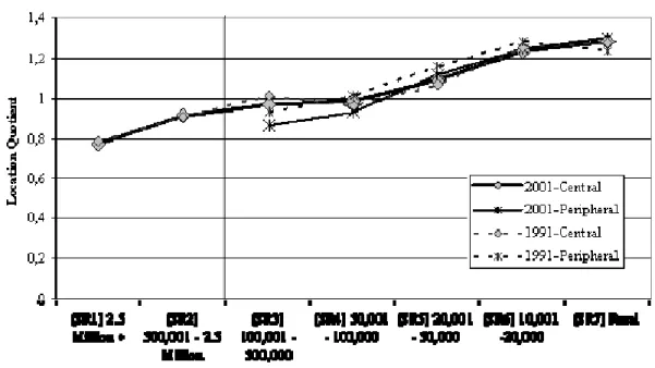
Moving to higher order services, the results for financial intermediation activities, Figure 12, and real estate, rental and business services, Figure 13, all clearly display a close fit to the hierarchical distribution model (Figure 5), with, however, a caveat: the periphery curve falls slightly below, and not above, the central curve.

Thus, for financial intermediation services, the distance effect is very weak (and in the “wrong” direction), although LQ values are greater for peripheral than for central areas for at least the SR3 class. The Spanish evidence that the “pure” distance effect is of little import for higher-order services is thus even stronger than in the Canadian case cited earlier. This suggests a truly hierarchical Christallerian distribution of service centres, where market size and the range of services are purely a function of city size. In the Spanish case, undoubtedly because peripheral distances are less, the distance-protection-effect seems to be inoperative, which is consistent with a symmetrical central place distribution of service centres. As a corollary, the size effect is very strong, with a clear downward slope for the central and peripheral curves over all classes. The metropolitan and primacy effects are also unambiguous, the highest for all sectors in 2001, and second highest (after real estate, rental, and business services) in 1991. In this respect, there is little evidence that agglomeration economies are any weaker in 2001 than in 1991 for most specialized services, suggesting again that IT has not fundamentally altered location choices.

(32)

Figure 12 - Financial Intermediation

Very similar behaviour is observed for real estate, rental and business activities (Figure 13). Accepting the distance caveat, the observed distribution clearly complies with the hierarchical model. The size effect is once again very strong, as are the primacy effect and the metropolitan effect, with a visible concentration in the major metropolitan areas. The

distance effect appears somewhat more important (but, remember, in the “wrong”

direction), its impact increasing as the size of the RS falls. This, together with a falling LQ for SR1 (a reduced primacy effect) suggests a crowding-out effect reminiscent of manufacturing. It is worth bearing in mind that this sector includes real estate and rental activities along with a mix of business services. If we could separate out higher-order business services, we would probably find a more dominant size effect and perhaps also a more consistent distance effect, as suggested by other studies on the service sector in Spain (Rubiera 2005). Regardless, our results suggest a crowding-out effect around the areas of Madrid and Barcelona, probably part of a larger process of metropolitan expansion and sprawl, where many of the services in question are following manufacturing to smaller

(33)

nearby communities. If so, we should not be surprised that the distance effect, as posited in the ideal model (Figure 5), does not hold for business services linked to manufacturing.

Figure 13 - Real Estate, Rental and Business Services

In summary, Figures 12 and 13 suggest that city size remains the fundamental factor determining the location patterns of financial and business services. This changes little from 1991 to 2001.

Turning to our last case, Figure 14 shows the spatial behaviour of the public sector as a whole (sectors L, M and N). These activities obey non-market criteria with respect to localization. Their spatial distribution is, however, a useful indicator of the redistribution effect of government activity. The clear winners are the largest peripheral cities. The high

LQ values for SR3 and SR4 are primarily due to cities that are the capitals of their province

or Autonomous Community, with a concentration of administrative and other public services. (Prime examples are: Santiago de Compostela, Valladolid, Logroño and Mérida).

(34)

Figure 14- Public Administration and Defense plus Education, Health and Welfare

(35)

Conclusion

A model for depicting the location of economic activity, initially devised for Canada, was applied to Spain. The model emphasises the role of city-size and of distance in explaining the spatial distribution of economic activity. The distributions observed for Spain were largely as expected, consistent with earlier applications to Canada, barring minor dissimilarities attributable mainly to the difference in size of the two countries. For given industries, the regularities observed for Spain with respect to the distance and the size variables were generally consistent with what location theory would lead us to expect.

We posited three stylized (ideal) location patterns, which, on the basis of our results, seem equally relevant to Spain. Higher-order services (finance and business services) show hierarchical distributions, where city-size is the overarching factor and distance (to a major metropolis) of little or no importance. Primary and resource-based industries display a counter-hierarchical distribution (called unbounded deconcentration), where both the distance and size effects push firms to more distant and smaller locations. Manufacturing follows what we call the constrained deconcentration model, in which firms favour small and medium-sized cities, close to major metropolitan areas. The crowding-out process appears to be in full swing in Spain during the 1991-2001 decade. None of this runs counter to classical location theory. Indeed, our results for Spain suggest that the basic economic principles constraining location choices, basically the trade-offs between agglomeration economies and diseconomies and the need (or not) to be close to a major urban area, continue to largely shape the location of industry, we are tempted to add, irrespective of national conditions.

In conclusion, our results, based on Spanish data for 1991 and 2001, provide new evidence that, on the whole, the location of economic activities continues to follow predictable patterns, consistent with location theory. By the same token, our results provide new evidence that distance continues to be a major factor constraining the location of industry. As in previous studies (of Canada and Mexico), distance was defined in terms of a one-hour travel radius from a major metropolis (of more than 500,000 inhabitants). This distance threshold appears to be no less relevant to Spain. We have explained the significance of this threshold by the continued (and perhaps growing) need of manufacturing firms to maintain

(36)

face-to-face contacts with producer service providers located in major metropolitan areas. We (like others) suggest that the arrival of new information technologies has not fundamentally changed this need. This also implies that great distances are not necessarily required to experience the negative effects of a “peripheral” location. Although large parts of Canada are truly peripheral, certainly when compared to Spain, the observed effect of a “distant” location, though not very distant (one hour’s drive), also appears in the Spanish case.

The patterns that emerge are quite stable over the decade under study. No major alteration in distributions is discernable. The two higher-order service classes, especially financial services, continue to display clear hierarchical distributions, reflecting the continued importance of agglomeration economies. The main observed changes may be interpreted in terms of the crowding-out effect (from large metropolitan areas), consistent with the rapid structural transformations of the Spanish economy during the 1991- 2001 decade.

(37)

References

Alonso, O; Chamorro, J. M. and González, X. (2004). “Agglomeration Economies in Manufacturing Industries: the Case of Spain,” Applied Economics, 36 (18). p. 2103-2116.

Beardsell, M. and Henderson, V. (1999). “Spatial Evolution of the Computer Industry in the USA,” European Economic Review, 43. p.: 431-456.

Cairncross, F. (2001). The Death of Distance 2.0. How the Communications Revolution

Will Change Our Lives. Norton.

Castells, M. (1996). The Network Society. Blackwell.

Coffey, W. J. and Polèse, M. (1988). “Location Shifts in Canadian Employment, 1971-1981, Decentralisation versus Decongestion,” Canadian Geographer, 32. p. 248-255. Duranton, G. and Puga, D. (2002). “Diversity and Specialization in Cities: Why, Where and

When Does it Matter,” in McCann, P. (Ed.), Industrial Localisation Economics. p. 151-186. Edward Elgar.

Gaspar, J. and Glaeser, E. (1998). “Information Technology and the Future of Cities,”

Journal of Urban Economies, 43. p. 136-156.

Ghemawat, P. (2001). “Distance still matters: the hard reality of global expansion,”

Harvard Business Review, September. p.: 131-147.

Glaeser, E. L. (1998). “Are Cities Dying?” Journal of Economic Perspectives, 12. p. 139-160.

Glaeser, E. L. (1994). “Cities, Information and Economic Growth,” Cityscape, 1 (1). p. 9-77.

Gordon, R. J. (2000). “Does the ‘New Economy’ Measure up to the Great Inventions of the Past?” Journal of Economics Perspectives, 14. p. 49-74.

Hall, P. (2000). “Creative Cities and Economic Development,” Urban Studies, 37. p. 639-649.

Henderson, J. V. (1997). “Medium Sized Cities,” Regional Science and Urban Economies, 27. p. 583-612.

INE (2004). Censo 2001, Resultados Detallados Definitivos. Instituto Nacional de Estadística. (http://www.ine.es)

INE (2002). Spanish National Accounts, 2001. Instituto Nacional de Estadística. (http://www.ine.es)

INE (1995). Censo 1991, Resultados Detallados Definitivos. Instituto Nacional de Estadística. (http://www.ine.es)

Ingram, G. K. (1998). “Patterns of Metropolitan Development: What Have we Learned?”

Urban Studies, 35. p. 1019-1035.

Kotkin, J. (2001). The New Geography: How the Digital Revolution is Reshaping the

(38)

MAP (2001). Informe sobre las Grandes Ciudades y Áreas de Influencia. Ministerio de Administraciones Públicas. (http://www.map.es)

Martínez, S. R. and Rubiera, F. (1999). “Identificación y Análisis de los Patrones Regionales de Terciarización de la Economía Española,” Economía Industrial, 328. p. 132-145.

MFOM (2004). Anuario Estadístico, 2003. Ministerio de Fomento. (http://www.mfom.es) Paluzie, E.; Pons, J. and Tirado, D. A. (2001). “Regional Integration and Specialization

Patterns in Spain,” Regional Studies, 35 (4). P. 285-296.

Polèse, M. and Champagne, E. (1999). “Location Matters: Comparing the Distribution of Economic Activity in the Mexican and Canadian Urban Systems,” International

Journal Science Review, 22. p. 102-132.

Polèse, M. and Sheamur, R. (2002). The Periphery in the Knowledge-Based Economy: The

Spatial Dynamics of the Canadian Economy and the Future of Non-Metropolitan Regions in Quebec and the Atlantic Provinces. INRS-UCS.

Polèse, M. and Sheamur, R. (2004). “Is Distance Really Dead? Comparing Industrial Location Patterns over Time in Canada,” International Regional Science Review, 27 (4). p. 1-27.

Polèse, M. (2005). “Cities and National Economic Growth: A Reappraisal,” Urban Studies, 42 (8). p. 1-24.

Porter, M. (1990). The Competitive Advantage of Nations. Free Press.

Roca, J. and Burns, M. C. (dir.) (2001). La Caracterización Territorial de las Áreas

Metropolitanas Españolas. Centre de Politica de Sól i Valoracions (CPSV) y Ministerio

de Medio Ambiente.

Rosenthal, S. and Strange, W. (2001). “The determinants of agglomeration,” Journal of

Urban Economics, 50. p. 191-229.

Rubalcaba, L. and Gago, D. (2003). “Regional Concentration of Innovative Business Services: Testing some Explanatory Factors at European Regional Level,” The Service

Industries Journal, 23 (1). p. 77-94.

Rubiera, F. (2005). Los Servicios Avanzados a las Empresas. Dinámicas de Localización,

Patrones de Externalización y Efectos sobre el Desarrollo Regional, Editorial Civitas.

Soto, J.; Pérez, J. and Feijóo, C. (2003). “Veinticinco Años de Sociedad de la Información en España. Evolución Tecnológica, Globalización y Políticas Públicas,” Economía

Industrial, 349-350. p. 63-82.

Trueba, M. C. and Lozano P. (2001). “Las Pautas de Localización Industrial en el Ámbito Municipal. Relevancia de las Economías de Aglomeración,” Economía Industrial, 337. p. 177-188.

(39)

Appendix A: The Definition of Urban and Metropolitan Areas

The Spanish Census provides population figures for each of the nation’s 8,036 municipalities. The data refer to the population with a principal residence within the municipality. The spatial classes used in this paper are based on this source, considering as urban all units with more than 10,000 inhabitants.

The Census also allows one to calculate the percentage of workers living in one municipality and working in another. Using this information, the Ministerio de Fomento (MFON, 2004) established a list of municipalities belonging to the key metropolitan areas. We used these lists to delineate the boundary areas of each relevant urban agglomeration (classes SR1, SR2, SR3 and SR4). The concept of metropolitan area used here refers to a large urban core municipality (more than 50,000 inhabitants) together with adjacent urban areas that have a high degree of social and economic integration with the urban core, with a total population of at least 500,000.

(40)

Appendix B: Sector Aggregation of the Database (Spanish

Census), The ISIC Rev. 3 Classification

A - Agriculture, hunting and forestry

01 - Agriculture, hunting and related service activities 02 - Forestry, logging and related service activities

B - Fishing

05 - Fishing, operation of fish hatcheries and fish farms; service activities incidental to fishing

C - Mining and quarrying

10 - Mining of coal and lignite; extraction of peat

11 - Extraction of crude petroleum and natural gas; service activities incidental to oil and gas extraction excluding surveying

12 - Mining of uranium and thorium ores 13 - Mining of metal ores

14 - Other mining and quarrying

D - Manufacturing

15 - Manufacture of food products and beverages 16 - Manufacture of tobacco products

17 - Manufacture of textiles

18 - Manufacture of wearing apparel; dressing and dyeing of fur

19 - Tanning and dressing of leather; manufacture of luggage, handbags, saddlery, harness and footwear

20 - Manufacture of wood and products of wood and cork, except furniture; manufacture of articles of straw and plaiting materials

21 - Manufacture of paper and paper products

22 - Publishing, printing and reproduction of recorded media 23 - Manufacture of coke, refined petroleum products and nuclear fuel 24 - Manufacture of chemicals and chemical products

25 - Manufacture of rubber and plastics products 26 - Manufacture of other non-metallic mineral products 27 - Manufacture of base metals

28 - Manufacture of fabricated metal products, except machinery and equipment 29 - Manufacture of machinery and equipment n.e.c.

30 - Manufacture of office, accounting and computing machinery 31 - Manufacture of electrical machinery and apparatus n.e.c.

32 - Manufacture of radio, television and communication equipment and apparatus 33 - Manufacture of medical, precision and optical instruments, watches and clocks 34 - Manufacture of motor vehicles, trailers and semi-trailers

35 - Manufacture of other transport equipment 36 - Manufacture of furniture; manufacturing n.e.c. 37 - Recycling

E - Electricity, gas and water supply

40 - Electricity, gas, steam and hot water supply 41 - Collection, purification and distribution of water

F - Construction

45 - Construction

G - Wholesale and retail trade; repair of motor vehicles, motorcycles and personal and household goods

50 - Sale, maintenance and repair of motor vehicles and motorcycles; retail sale of automotive fuel 51 - Wholesale trade and commission trade, except for motor vehicles and motorcycles

52 - Retail trade, except for motor vehicles and motorcycles; repair of personal and household goods

H - Hotels and restaurants

55 - Hotels and restaurants

I - Transport, storage and communications

60 - Land transport; transport via pipelines 61 - Water transport

62 - Air transport

63 - Supporting and auxiliary transport activities; activities of travel agencies 64 - Post and telecommunications

J - Financial intermediation

65 - Financial intermediation, except insurance and pension funds 66 - Insurance and pension funds, except compulsory social security 67 - Activities auxiliary to financial intermediation

K - Real estate, renting and business activities

70 - Real estate activities

71 - Renting of machinery and equipment without operator and of personal and household goods 72 - Computer and related activities

(41)

73 - Research and development 74 - Other business activities

L - Public administration and defence; compulsory social security

75 - Public administration and defence; compulsory social security

M - Education

80 - Education

N - Health and social work

85 - Health and social work

O - Other community, social and personal service activities

90 - Sewage and refuse disposal, sanitation and similar activities 91 - Activities of membership organizations n.e.c.

http://unstats.un.org/unsd/cr/registry/regcs.asp?Cl=2&Lg=1&Co=92 92 - Recreational, cultural and sporting activities

93 - Other service activities

P - Private households with employed persons

95 - Private households with employed persons

Q - Extra-territorial organizations and bodies

(42)

Appendix C: Descriptive Statistics

Size Effect (Slope)

Central SRs Peripheral SRs Ultra-Peripheral SRs

Sectors following the ISIC Rev. 3

Classification _{1991 2001 ∆} _{1991 2001 ∆} _{1991 2001 ∆}

A – Agricultural, hunting and

forestry -37.2216 -42.5963 -5.3746 -39.1117 -39.9827 -0.8710 -47.7378 -47.8252 -0.0874

B – Fishing 9.6695 -0.5449 -10.2144 -104.0114 -160.1758 -56.1644 -117.8653 -196.9472 -79.0818

C – Mining and quarrying -10.4525 -10.2220 0.2304 -84.4137 -147.9957 -63.5820 -90.4391 -159.1642 -68.7251

D – Manufacturing -4.5119 -7.6638 -3.1519 1.0363 -5.8372 -6.8734 -11.5555 -21.4856 -9.9301

E – Electricity, gas and water

supply 4.0794 1.2419 -2.8374 0.8342 -11.7110 -12.5451 14.7571 -4.0582 -18.8153

F – Construction -8.1249 -8.8252 -0.7003 -11.8134 -12.7557 -0.9423 -12.0213 -5.6355 6.3859

G – Wholesale and retail trade;

repair of motor vehicles, motorcycles and personal and household goods

5.1794 3.3888 -1.7905 2.6832 1.6637 -1.0196 11.0333 6.2821 -4.7512

H – Hotels and restaurants 9.4198 10.5550 1.1352 -0.9366 -0.7776 0.1591 35.4134 29.7153 -5.6981

I – Transport, storage and

communications 11.8470 6.4986 -5.3484 5.9898 4.8763 -1.1135 25.1249 19.2501 -5.8748

J – Financial intermediation 13.2529 9.3602 -3.8926 14.2999 15.9929 1.6930 14.8553 10.4692 -4.3861

K – Real estate, renting and

business activities 17.4441 11.8786 -5.5655 13.4229 14.4538 1.0309 24.4008 17.6231 -6.7777

L – Public administration and

defence; compulsory social security

9.3878 6.4385 -2.9493 22.8972 17.9107 -4.9864 17.9769 12.3900 -5.5868

M – Education 6.2094 5.5044 -0.7050 16.3671 15.7167 -0.6504 13.0545 7.5323 -5.5222

N – Health and social work 21.0631 13.7253 -7.3379 30.6008 20.5417 -10.0591 22.7989 13.7879 -9.0109

O & Q – Other social and

personal services activities & Extra-territorial organizations and bodies (*)

10.6448 -21.5772 -32.2220 11.0261 -45.1602 -56.1864 20.8025 -10.5464 -31.3489

P – Private households with

(43)

Distance Effect Metropolitan Effect Primacy Effect Rural Effect 1991 2001 ∆ 1991 2001 ∆ 1991 2001 ∆ 1991 2001 ∆ A -0.3734 -0.3190 0.0543 0.1280 0.3235 0.1955 0.2469 0.2365 -0.0104 3.4199 2.5681 -0.8518 B -0.7309 -2.0775 -1.3465 0.1519 0.0878 -0.0642 0.8304 0.2343 -0.5961 0.4976 0.6301 0.1325 C -0.6572 -1.4367 -0.7795 0.6271 0.3380 -0.2890 0.3213 0.0938 -0.2274 1.8516 2.2269 0.3753 D 0.3325 0.3088 -0.0237 1.1406 0.8459 -0.2947 1.1495 1.0813 -0.0681 0.9005 1.1013 0.2008 E -0.0726 -0.1422 -0.0696 1.0487 0.9231 -0.1256 1.1650 0.9897 -0.1753 0.9414 0.9617 0.0204 F -0.0224 0.0320 0.0544 0.7093 0.7042 -0.0051 0.8644 0.8509 -0.0134 1.2129 1.2792 0.0663 G -0.0244 -0.0319 -0.0075 0.9500 1.0183 0.0684 0.8775 0.8859 0.0084 0.6533 0.8177 0.1644 H 0.0908 0.1145 0.0237 0.8600 0.8820 0.0220 0.9550 0.9296 -0.0254 0.9256 0.9788 0.0532 I -0.0803 0.0009 0.0811 1.2407 1.5130 0.2723 1.1470 1.2883 0.1413 0.7426 0.8608 0.1182 J 0.0540 0.0074 -0.0466 1.4500 1.5079 0.0579 1.5011 1.5081 0.0069 0.5257 0.6288 0.1031 K 0.1553 0.1096 -0.0457 1.7672 1.5608 -0.2064 1.5389 1.4072 -0.1318 0.3929 0.5536 0.1608 L -0.1811 -0.2522 -0.0711 0.8716 0.9219 0.0502 0.9830 0.8571 -0.1259 0.5877 0.8166 0.2289 M -0.1676 -0.1657 0.0019 0.9017 0.9609 0.0591 0.8472 0.8401 -0.0071 0.6297 0.6609 0.0312 N -0.1854 -0.1687 0.0167 0.8942 0.9375 0.0432 0.8523 0.8723 0.0200 0.4411 0.5940 0.1528 O&Q 0.0984 -0.1733 -0.2716 1.2845 0.1311 -1.1534 1.2076 1.0096 -0.1981 0.6122 0.4606 -0.1516 P -0.0920 0.0034 0.0954 1.0960 1.4300 0.3340 1.1298 1.4052 0.2754 0.7566 0.7298 -0.0267

(44)

Central Rural Effect _{Specificities Effect}Ultra-Peripheral Main Ultra-Peripheral _{Cities Effect} Ultra-Peripheral Rural Effect 1991 2001 ∆ 1991 2001 ∆ 1991 2001 ∆ 1991 2001 ∆ A 0.5813 0.5369 -0.0444 0.4490 0.7004 0.2514 0.2850 0.4648 0.1798 0.4421 0.3173 -0.1248 B 1.4077 0.4944 -0.9133 0.5884 1.3395 0.7511 0.6699 0.4912 -0.1787 2.2954 0.5302 -1.7652 C 0.7074 0.4770 -0.2304 0.6768 0.9051 0.2283 0.9839 0.6290 -0.3549 0.2448 0.1627 -0.0821 D 1.7468 1.4184 -0.3285 0.5973 0.7473 0.1500 0.9915 0.9764 -0.0150 0.6448 0.4395 -0.2052 E 0.8511 0.8072 -0.0438 -0.2817 -0.1184 0.1633 1.0104 0.9322 -0.0782 1.4161 1.0180 -0.3981 F 1.0366 0.9845 -0.0521 -0.0043 -0.1184 -0.1141 0.6294 0.7398 0.1104 1.2928 1.2370 -0.0558 G 1.2563 1.1458 -0.1104 -0.2164 -0.0735 0.1429 0.8791 1.0598 0.1807 1.5112 1.2475 -0.2637 H 0.9168 0.9245 0.0077 -1.6341 -1.3718 0.2623 0.5378 0.5315 -0.0063 3.1726 2.8577 -0.3149 I 1.0323 1.1014 0.0691 -0.3125 -0.1985 0.1140 1.4443 1.3826 -0.0618 1.3708 1.3209 -0.0500 J 1.2374 1.2760 0.0386 0.1268 0.1732 0.0464 1.5649 1.5015 -0.0634 1.2412 1.0916 -0.1496 K 1.7065 1.4574 -0.2491 -0.1513 -0.0476 0.1037 1.2872 1.2467 -0.0404 2.4818 1.5064 -0.9755 L 0.9864 0.8724 -0.1140 -0.6430 -0.7803 -0.1372 0.3260 0.2804 -0.0456 1.3102 1.2529 -0.0573 M 1.0255 1.1264 0.1009 0.0125 0.0697 0.0573 1.0317 0.8387 -0.1930 1.3960 1.3457 -0.0503 N 1.0381 1.0730 0.0349 0.0468 0.0634 0.0167 0.9007 0.8823 -0.0184 1.1373 1.1411 0.0038 O&Q 1.3460 1.3693 0.0232 -0.2504 -7.1797 -6.9294 1.0955 0.0760 -1.0195 1.5942 10.0845 8.4904 P 0.8243 0.8952 0.0709 0.0059 0.0924 0.0865 0.8343 1.2089 0.3745 0.8790 1.0093 0.1303

(*) In the 1991 Census, branches O and Q are combined. The 2001 Census distinguishes between them but, in order to allow comparison, the descriptive statistics are calculated together at both times.