Design of a precise X-Y-Theta nanopositioning optical sensor

(1)

Design of a Precise X-Y-Theta

Nanopositioning Optical Sensor

by

Michael B. Johnson

Submitted to the Department of Mechanical Engineering

in partial fulfillment of the requirements for the degree of

Bachelor of Science in Mechanical Engineering

at the

MASSACHUSETTS INSTITUTE OF TECHNOLOGY

June 2009

@Copyright Massachusetts Institute of Technology, 2009.

All rights reserved.

Author ...

Departmk.Q A 4echanical Engineering

May 11, 2009

N

ciT>l~

/1

Certified by...

Brian W. Anthony

Research Scientist

Thesis Supervisor

Accepted

by ...

_{John H. Lienhard V}

Chairman, Department Committee on Undergraduate Theses

MASSACHUSETTS INSTITUTE OF TECHNOLOGY

SEP

16 2009

LIBRARIES

(2)

(3)

Design of a Precise X-Y-Theta

Nanopositioning Optical Sensor

by

Michael B. Johnson

Submitted to the Department of Mechanical Engineering on May 11, 2009, in partial fulfillment of the

requirements for the degree of

Bachelor of Science in Mechanical Engineering

Abstract

A position measurement system was designed to estimate the absolute and relative position of an x-y-O nanopositioning stage for use in the metrology of microfluidic devices during and after manufacturing. The position sensing system consists of a visible-light high-speed area camera, a target pattern, and image processing software. The target pattern consists of a square grid with unique binary codes in each square that identify the square's global position in the grid.

In macroscopic-scale testing of the position sensing system, the angular orientation of the target pattern was successfully measured with less than one degree uncertainty. However this uncertainty is several orders of magnitude larger than the target preci-sion of the sensor, and it is still unclear whether sufficient precipreci-sion is attainable with this system and software.

This thesis also describes a previous attempt to perform this metrology using consumer-grade contact image sensor scanners, other elements of the current metrol-ogy system design, and the non-orthogonal viewing angle concept, which is the fun-damental underpinning of the microfluidic metrology system as a whole.

Thesis Supervisor: Brian W. Anthony Title: Research Scientist

(4)

(5)

Acknowledgments

This work would have been impossible without the insight and support of Dr. Brian Anthony, my thesis advisor, who has supervised my work on this project since I joined his group as a UROP student at the beginning of 2008. Dr. Anthony has done an excellent job at making his time and resources available to me, and has consistently reminded me of how my project fits into the work of the larger research group. Also, Dean Ljubicic has been invaluable for his guidance in shaping the direction of this project and bringing new ideas to the table. Both gentlemen are skilled and patient teachers, and a pleasure to work with.

I would also like to acknowledge Brian Syverud and Salman Aldukheil, my UROP partners at the start of this project, along with the researchers in the Center for Polymer Microfabrication and the Laboratory for Manufacturing and Productivity at large who have spared a moment to help me along the way. Outside of Building 35, I would like to thank my parents, my neighbors in French House, and everybody else who has offered advice, or has been a sounding board for new ideas.

(6)

(7)

List of Figures

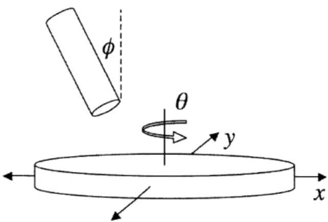
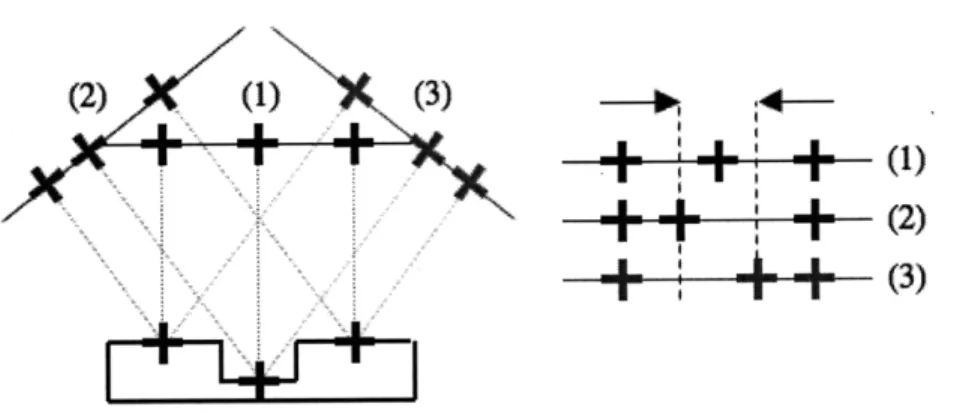
1-1 An x-y-O stage sits beneath the lens of a high-speed area camera. The lens is fixed in space, tilted at an angle, 0, from normal to the stage. 14 1-2 Schematic of the non-orthogonal viewing angle concept. The center

fiducial appears to shift when the angle changes because it is at a different depth than the others. ... .. 16

2-1 The basic layout of a contact image sensor (CIS) scanning element. . 18 2-2 Two halves of non-orthogonal viewing angle scans are mated. The top

and bottom line up between the two halves, but discontinuities in the markings at the center indicate that the center is at a different depth from the top and bottom. ... ... 20

3-1 A camera mounted non-orthogonally above the stage images the sam-ple through a telecentric lens, while an identical camera with a non-telecentric magnifying lens images the position sensor target pattern which is located on the underside of the stage. . ... . 24 3-2 A telecentric lens has an infinite focal length, so images are magnified

without any radial distortion. ... ... .. . . 25 3-3 The image of a square array of dots is not distorted by a telecentric

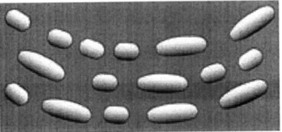
lens; however, radial distortion is apparent in a non-telecentric lens. . 25 3-4 DVD pits and lands have a minimum length of 0.4 microns and a track

pitch of 0.74 microns. The shapes of the pits are slightly irregular, and they are laid out on a spiral path. ... ... . . . 27

(10)

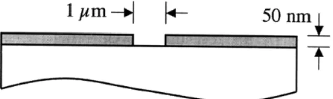
3-5 A 50-nanometer thick layer of gold or chrome is deposited on a glass substrate. Areas with dimensions as small as one micron are electron-blasted out, creating a pattern on the surface. ... . . 28

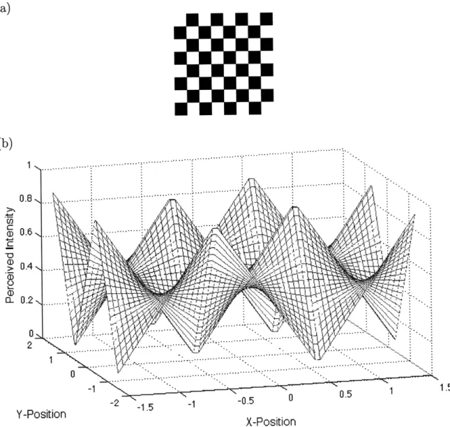
4-1 (a) A single-pixel sensor moves across the periodic pattern shown at the bottom of the chart. The intensity perceived by the pixel is equivalent to the area fraction beneath the pixel that is white when the pixel is centered at a given position. (b) A sensor with two side-by-side pixels moves across the same pattern as in (a). . ... 30 4-2 (a) A two-dimensional checkerboard pattern. (b) The intensity

per-ceived by a single-pixel sensor as a function of the position of the center of the pixel. ... ... 31 4-3 This absolute linear position encoder uses two scales that are read

simultaneously. The top scale is a pseudo-random binary sequence that gives absolute position, and the bottom scale is a periodic scale for fine positioning relative to the absolute scale. ... 32 4-4 A square grid provides relative positioning around six-by-six global

positioning arrays that indicate the orientation of the grid and the absolute position of the square in the grid at large. . ... 33 4-5 A Data Matrix is a type of barcode that can encode far more characters

than a UPC barcode, and can encode any ASCII character, not just numbers. This Data Matrix encodes "Design of a Precise X-Y-Theta Nanopositioning Optical Sensor." ... . 34 4-6 Layout key for the global positioning arrays that add absolute position

information to the sensor target pattern. .. ... 34

5-1 Maximum frame size is required when the stage is rotated by a multiple of 45 degrees from the camera frame. A square frame with side of length 45 microns ensures that at least one full grid box is always present in the frame. .... ... ... . ... .. 37

(11)

5-2 The raw image from the camera (a) is cropped and inverted, and the grayscale is transformed to use the full possible range (b). . ... 39 5-3 The match field for the image against a 4-by-4 kernel of ones is plotted.

Low-match data has been removed. . ... 40 5-4 A two-dimensional representation of the match matrix when the image

is filtered with a 4-by-4 kernel of ones. Darker grays correspond to stronger matches. Weak match areas have been removed. ... 41 5-5 The Hough transform identifies lines by polar parameters that describe

the perpendicular distance, p, and direction, 0, of the line (bold) from the origin. ... ... .. 41 5-6 The Hough transform accumulates image points in a polar parametric

space. It then identifies the points of peak density (the eleven box markers). These peaks correspond to probable lines in the image. . . 42

(12)

(13)

Chapter 1 Introduction

The objective of the project is to design an optical position sensor, consisting of a camera and target pattern, that can determine the position and orientation of an x-y-O stage with a target resolution of 50 nanometers in the x- and y-directions, and 0.1 arc seconds in the 0-direction, with an 8-inch diameter circular range.

1.1 Application to Microfluidic Device Metrology

An x-y-O nanopositioning stage is being developed for use in the metrology of mi-crofluidic devices. The stage will be located beneath a high-speed area camera which will be tilted so that the lens axis is not normal to the stage plane, as shown in Fig-ure 1-1. The stage will allow full in-plane manipulation of an 8-inch diameter wafer sample. To achieve precise positioning of the stage, the stage actuators will receive continuous position feedback from the optical position sensor.

1.1.1 The Center for Polymer Microfabrication

The Center for Polymer Microfabrication (CPM) is a collaboration between the Lab-oratory for Manufacturing and Productivity at MIT and the Biochemical Process Engineering Laboratory at NTU in Singapore. The center's goal is to develop and optimize processes for manufacturing polymer-based microfluidic devices with micron

(14)

Figure 1-1: An x-y-O stage sits beneath the lens of a high-speed area camera. The lens is fixed in space, tilted at an angle, b, from normal to the stage. The stage allows full rotation and translation of an eight-inch diameter circular sample.

and sub-micron scale channels, that would be appropriate for inexpensive, large-scale commercialization.

1.1.2 Functional Requirements

Metrology is critical in the development of any manufacturing system, since it is necessary to verify the quality of the manufactured parts. For a metrology system to be useful in microfluidics manufacturing, the system must be able to:

* measure three-dimensional features;

* measure the size and location of features;

* measure with sub-micron precision; and

* perform all measurements quickly over a large area, making the system practical for post-process and in-process metrology.

No measurement system is currently available commercially that meets all of these functional requirements.

1

(15)

1.1.3 Previous System

The previous system used by the CPM for measuring microfluidic devices was a ZYGO white light interferometer. Though the ZYGO measures three-dimensional features with the requisite precision, it is inadequate because it takes far too long to take its

measurements, making it impractical for use on a production line.

1.2 Non-Orthogonal Viewing Angle Concept

In order to achieve three-dimensional metrology from a two-dimensional camera im-age, the viewing angle is tilted away from orthogonal with respect to the sample plane. By changing this viewing angle, features at different depths on the sample are perceived to shift in the images, as shown in Figure 1-2. The depth of a feature, D,

is

D = 2tan' (1.1)

2 tan 0'

a function of the size of the shift, 6, and the viewing angle, 0, away from orthogonal. For a given viewing angle, the image shift varies linearly with the feature depth.

To obtain a depth measurement, a minimum of two images are required for com-parison (additional images would allow error reduction). The simplest pair of images are taken with viewing angles of 0 and -0, as is the case in Figure 1-2. This change in angle can be achieved through three primary methods:

* changing the image sensor angle to the other side of normal over a fixed sample; * using two image sensors, fixed at opposite angles, above a fixed sample; or * rotating the sample 180 degrees in its plane under a fixed image sensor.

The price of a second image sensor (for use at the scale and precision of this project) makes the second option impractical, so the remaining options are moving the sensor or moving the sample. Because the sample must be inserted and removed from the metrology device in any case, some method of fixturing the sample must be provided. Also, the system must be able to move the image frame to different parts of the

(16)

sample. It was decided that combining all positioning flexibility in the sample stage was the best solution, leaving the image sensor fixed at a non-orthogonal angle to the image plane.

(2) (1 3)

4--(2)

Figure 1-2: A sample channel (left) has three fiducial marks-one in the bottom of the channel, and one on each side-such that the fiducials appear equally spaced in an orthogonal view (1). When viewed from a non-orthogonal angle (2, 3), the center fiducial, which is at a different depth than the other two fiducials, appears to shift to the side. The three images are compared (right) and the shift measured. Adapted

from [Johnson 2008].

1.3 Super-Resolution

Information is distorted and aliased when an image is captured because each pixel's intensity (and hue, for color images) is the average intensity of the area beneath the pixel. When it is necessary to generate an image with higher resolution than the camera and lenses are capable of producing, it is possible to use super-resolution image processing software to obtain sub-pixel intensity information.

Super-resolution works by comparing multiple images of the same object where each image capture is identical except for a sub-pixel translation in the object position between frames. Since the divisions between pixels on the object have shifted slightly from one frame to the next, the information is grouped differently, and the aliasing is changed. By comparing the images, the software can reconstruct fine sub-pixel detail and construct an image with increased resolution.

(17)

Chapter 2 Scanner Modification Project

In spring 2008, a first attempt at three-dimensional metrology using the non-orthogonal viewing angle concept was made with modified consumer-grade flatbed contact image

sensor (CIS) scanners. Financially, using these 100-dollar instruments in conjunction with the necessary image processing software would make the metrology system much more affordable than the 60,000-dollar instruments intended for three-dimensional imaging of microscale samples [Johnson 2008]. The project was successful as a proof-of-concept experiment; however, the scanners could not achieve the required image clarity or resolution to be useful at the scale and precision of microfluidic devices.

2.1 Macroscopic Test Channels

The objective of the scanner modification project was to prove the non-orthogonal viewing angle concept for channel depths as small as 0.01 inches. If this phase had been successful, the technology would have been adapted to the smaller scale of microfluidic devices. The test samples used in the scanner project were "macro channels"--layers of Scotch tape on a plastic slide. Scotch tape is precisely 0.0020 ± 0.0001 inches thick (estimated uncertainty), so stacked layers of Scotch tape make a very repeatable channel depth.

(18)

2.2 CIS Scanners

A contact image sensor consists of a linear array of image sensors beneath a linear array of cylindrical one-to-one lenses. The sensor sweeps beneath the glass scanner bed, as shown in Figure 2-1, assembling an image line by line. CIS scanners were used for this project instead of classic charge-coupled device (CCD) scanners, since the optical path length and path angle with respect to the image plane are relatively constant across the width of the linear scanner. Classic CCD scanners collect light from the full width of the image to a narrow sensor at the center of the scanner. The uniform optical path of a CIS scanner allows us to modify the viewing angle without worrying about inherent edge effects in the CCD sensor.

Light guide

Image sensor 4

Figure 2-1: The basic layout of a contact image sensor (CIS) scanning element. This linear image sensor travels back and forth under the glass of the scanner bed

[Epson 2005].

The Canon LiDE 90 CIS scanner was selected for modification and testing in this project. Each scanner cost 80 dollars, and the design seemed more easily modified than other models. The advertised maximum resolution for this scanner was 2400 dots

(19)

2.3 Scanner Modifications

The primary modification made to the Canon LiDE 90 scanner in this project was to rotate the sensor assembly by 15 degrees about the principal axis of the sensor to create a non-orthogonal viewing angle for the sensor. To provide clearance for this rotation, the glass was raised slightly and remounted on the scanner, a portion of the sensor assembly (not containing functional elements) was milled away, and the plastic sliding bearing surfaces, which previously kept the sensor assembly aligned to the plane of the glass, were removed. The sensor assembly was supported in its rotated position by two springs, which pressed the top edge of the sensor against the underside of the glass.

To align parts on the scanner bed, a ruled rectangle was affixed to the glass. The smaller rectangular samples were aligned by pushing one corner of the sample into the corner of the ruled rectangle.

2.4 Results

The macro channels were scanned, rotated 180 degrees, and rescanned to generate images with views of 15 and -15 degrees from normal. These two images were aligned to each other and superimposed to observe the shift in the location of the center marks. Figure 2-2 shows a composite image of the sample, with the left half of the image from one orientation, and the right half of the image from the the rotated orientation. The marks on the outside surfaces line up in the two halves, but there is a discontinuity in the marks on the bottom of the channel. This shift in the image indicates that the center of the image is in a different plane than the top and bottom of the image.

Figure 2-2 constitutes a successful proof-of-concept for non-orthogonal viewing an-gle depth perception, however the image quality problems-fuzziness and vertical streaking-make this modified scanner unsuitable for the smaller-scale geometries of

(20)

Figure 2-2: Two halves of non-orthogonal viewing angle scans of a 0.030-inch deep channel are mated (separated by the heavy black line). Each scan was rotated 180 de-grees from the other. The top and bottom line up between the two halves, but dis-continuities in the markings at the center indicate that the center is at a different depth from the top and bottom. Note that the shadow line at the channel border

(21)

* an increased distance from the top of the lens array to the image plane, resulting from raising the glass and tilting the sensor assembly;

* vibrations in the whole system due to the slow stepping motion of the carriage when scanning at high resolution (native to the unmodified scanner); and * vibrations in the carriage movement after the four-point sliding contact bearings

were removed, leaving the leading edge of the sensor assembly as the bearing surface.

Since the first two error sources were not resolvable without a major rebuild of the scanner, the scanner modification project was abandoned.

2.5 Use Conditions

Even if the image quality produced by the modified scanner were adequate for measur-ing microfluidic devices, the device was still not well suited for use on a microfluidics manufacturing line. The scanner project was one facet of the CPM's puFac (as in "Micro-Factory") project, an interdisciplinary collaboration to develop a functional teaching factory for microfluidic devices. Two scanners were incorporated for in-process metrology. The Takt time for this production line was set at less than four minutes [Hardt 2008]; however, the scanner needed over two minutes to scan the 10 square inch area of the ruled rectangle in 8-bit grayscale at a resolution of 2400 dots per inch, and since a minimum of two scans1 are necessary to make depth measure-ments of the part, the scanning process was not fast enough for use on the production line.

In addition, the scanning system requires that the part be repositioned on the scanner bed between each scan. This line was designed to be operated with a single robotic arm that would not have time to return to the scanner multiple times each cycle, so a means of manipulating the sample on the scanner bed would have been necessary.

(22)

2.6 Scanner Project Conclusion

The scanner modification project showed that the non-orthogonal viewing angle con-cept can be used to measure depth, however the Canon LiDE 90 was not appropriate for imaging microscale samples. A higher resolution or higher precision system was necessary. In addition, the imaging system needed to be faster and the metrology system needed the ability to manipulate the part independently of the rest of the system.

(23)

Chapter 3 X-Y-8 Stage with Area Cameras

After the consumer-grade scanners were shown to be inappropriate for imaging mi-crofluidic devices, the project shifted to designing a better scanning system from the ground up. The system consists of an x-y-O stage with an optical target pattern on the bottom for position sensing, and fixturing on top for microfluidic devices. Two identical high-speed area cameras with different lenses are mounted above and below the stage as the image sensor and position sensor, as shown in Figure 3-1. The cam-eras are fixed in space, and the stage moves, scanning the samples under the camera lenses.

3.1 The Stage

The stage is being designed by Dean Ljubicic. The first iteration of the stage will be constructed from off-the-shelf parts, including air bearings to support the motion in x and y, and a stepper-motor-actuated turntable to allow rotation in 0. Subsequent designs may include a magnetically levitated stage, or a magnetically positioned stage levitated on an air table.

When designing a positioning system for this stage, the first idea that comes to mind is a series of three position encoders-a linear encoder on each of the x- and y-axes, and a rotary encoder on the 0-axis. However, serial measurements, where each encoder measures with respect to the previous, are not precise enough for this

(24)

appli-Figure 3-1: A camera mounted non-orthogonally above the stage images the sample through a telecentric lens, while an identical camera with a non-telecentric magnifying lens images the position sensor target pattern which is located on the underside of the stage.

cation, since errors in each stage and encoder level are accumulated in the combined measurement. Instead, parallel measurements must be made to determine the stage position. In other words, all measurements must be made from ground (where the cameras are fixed) directly to the position of the sample stage, without intermediate steps.

Using a parallel measurement system has the added advantage that the accuracy of the stage can be reduced, as long as the positioning sensor and control system are able to perceive and compensate for the systematic errors.

3.2 The Cameras

Both cameras will be high-speed area cameras, capable of taking images at up to 30,000 frames per second. However the sample camera and the positioning camera will be set up and used differently.

(25)

3.2.1 The Sample Camera

The sample camera will be mounted non-orthogonally and will be used to scan mi-crofluidic samples, just as the flatbed scanners did before. CIS scanners use a line camera to scan one row of pixels at a time, and this sample camera will be used similarly: the whole field of the camera will not be used, rather just one to three lines of pixels from the center of the sensor.

The lens on the sample camera will be telecentric (see Figure 3-2), transmitting a one-to-one image without the radial distortion inherent in non-telecentric lenses (see Figure 3-3). The telecentric lens provides a 200-micron depth of field, which is significantly greater than the depths of the microfluidic channels it will be imaging, allowing the top and bottom of the channels to be in focus simultaneously.

I

. .

I

IIini

-Figure 3-2: A telecentric lens has an infinite focal length, so images are magnified without any radial distortion [Telecentric].

*e *0. 6...

99

t t ****.

#* ***0*** 9 * # 9 *

Figure 3-3: The image of a square array of dots is not distorted by a telecentric lens (left). However radial distortion is apparent in a non-telecentric lens (right). Note how the principal axes experience minimal distortion, but the distortion increases as you move away from the axes [Telecentric].

In addition, the lack of radial distortion means that the lines in the camera sensor can be used interchangeably (as opposed to a non-telecentric lens where the distortion

(26)

increases in severity with distance from the lens axis). As a result, samples of different thicknesses, or samples that have bowed so that they are no longer flat, can be imaged by selecting rows of the camera sensor that are higher or lower to change the path length and keep the sample within the image field. With a non-telecentric lens, the radial distortion would limit use to only the center line of the lens, so a vertical adjustment axis would need to be added to the stage or sample camera mount.

The advantage of a non-telecentric lens is 0.5-micron resolution, which is sufficient for our applications, since it matches the camera pixel size. The telecentric lens, on the other hand, has only 3.5- to 7-micron resolution, and will require additional image processing for super-resolution.

3.2.2 The Positioning Camera

The positioning camera reads the glass pattern (described in Chapter 4) on the un-derside of the stage to determine the orientation and position of the stage. This camera uses a non-telecentric lens which magnifies the pattern image fourteen times, such that one pixel corresponds to 0.5 microns on the pattern.

3.3 The Position Sensor Target

The position sensor target is mounted on the underside of the stage. As the stage moves, the target moves through the field of view of the positioning camera, which tracks the motion of the target pattern. The target is illuminated from below, and the light is absorbed by the target or reflected into the camera. The sensor target provides relative and absolute position and rotation of the 8-inch diameter circular stage throughout its full range of motion.

3.3.1 DVD Technology

The first technology that was considered for writing and reading optical patterns at this scale was DVD technology. DVDs store information in a series of pits and

(27)

lands on a spiral track (see Figure 3-4). These pits are made with better than 50-nanometer precision [Taylor 2006], which is this project's linear resolution goal. In Blu-Ray Discs, the pits themselves can be as small as 0.138 microns, with a track pitch of 0.32 microns, which is half that of the DVD's [Taylor 2004]. Although the pit lengths are very precise, Figure 3-4 shows that pit width and shape are highly irregular. This, plus the spiral path, makes DVD technology inappropriate for this application.

Figure 3-4: DVD pits and lands have minimum length of 0.4 microns and a track pitch of 0.74 microns. The shapes of the pits are slightly irregular, and they are laid out on a spiral path. The path curvature in this image is exaggerated for clarity [RPA].

3.3.2 Photolithography Technology

A more flexible alternative to DVD technology is photolithography masks which can be customized to a wide range of geometries. In photolithography, a 50-nanometer thick layer of chrome or gold is deposited on a substrate of soda-lime glass or fused-quartz glass (see Figure 3-5). These substrates are chosen for their extremely low coefficients of thermal expansion-8.6 x 10-6 per Kelvin [VDC 2008] and 5.5 x 10-7 per Kelvin [TGP 2008], respectively-so that the dimensions of the substrate and resultant accuracy of the position sensor are independent of temperature variations. Portions of the top layer are removed by electron blasting, leaving a pattern on the substrate. The removed areas can have dimensions as small as one micron, and

appear black. One manufacturer of stock and custom photolithography masks is Applied Image, Inc., of Rochester, New York.

(28)

1m- 50 nm

T

Figure 3-5: A 50-nanometer thick layer of gold or chrome is deposited on a glass substrate. Areas with dimensions as small as one micron are electron-blasted out, creating a pattern on the surface. Note: this figure is not drawn to scale.

(29)

Chapter 4 Sensor Pattern

A pattern was developed for the sensor target that allows for relative and absolute position sensing, using a square grid of lines and global positioning codes within each grid box to identify the box's absolute location.

4.1 Relative Positioning

The simplest case of relative positioning is that of a linear encoder with a single-pixel sensor. The pattern used is a periodic black-white pattern where the half-period is the same width as the pixel. As the pixel moves over the pattern, the intensity perceived by the pixel (the fraction of the area beneath the pixel that is white) varies as shown in Figure 4-la. Though the actual change in intensity is continuous, the pixel perceives the intensity in quantized grayscale. Therefore, the sensor, imaging in n-bit grayscale, can discern 2" locations in each half period of the pattern.

The one-pixel sensor cannot uniquely identify each point over a full period. For example, if the intensity is 1, the sensor knows it is centered on a white segment, however if the intensity begins to decrease, the sensor does not know which way it is traveling. To correct this, a second pixel is added beside the first, so that there is a phase shift in the intensities perceived by each pixel (Figure 4-1b), allowing unique positioning within each period.

(30)

pat-(a) ++ ++ -I-.. t-+4-+ -t-++ ++ ++ -2 -1.5 -1 -0.5 0 0.5 1 1.5 2 Position (b) + S++ * * * ** * * * * ++-t+++ + LeftPixel *, -m-+, * + -* Right Pixel + * + + * + ++ * --+ * + + 4, + -H 44 -4 -I-I- 44444444444 -2 -1.5 -1 -0.5 0 Position 0.5 1 1.5 2

Figure 4-1: (a) A single-pixel sensor moves across the periodic pattern shown at the bottom of the chart. The pattern has a period of length of 2, and the pixel has length of 1. The intensity perceived by the pixel is equivalent to the area fraction beneath the pixel that is white when the pixel is centered at a given position. (b) A sensor with two side-by-side pixels moves across the same pattern as in (a). Each pixel has a length of 0.5, so the overall size of the sensor is unchanged. Here, position refers to the location of the border between the pixels. For clarity of the figures, reduced resolution (3-bit grayscale) and increased position increment (0.05) are used. Unlike

(a), (b) has a unique perception of each position over the period of the pattern.

1 0.6 0.4 S0.2 0.8 -0.6 0.4

(31)

-tern (Figure 4-2a). The intensity field perceived by a single pixel is shown in Fig-ure 4-2b, and as before, multiple pixels are required to uniquely identify each point in one period of the pattern.

(b) .. .. .. .. . .. .. .. .. .... .. .. . .. .. .. . . . .•. .. . .. . .. .. .. . .. . ... . .... .. . .. .. .. . ... .. ... .. .. •. .. .. . .... ... .. / ," , .. . 0.8 ... ... ... ) 0.6 -. .... .. , > 0.4 L... a- 0.27. 0) Y-Position N₁ 05 0 05~ 2N N (A _{It AZ /Y ...} _...._' ... Position° _¥ _{, i}.:..._... _' ... . .. .' . . . .. .... . . . .... . . ... ... " .~~~ .. • . . . , . . .. . . . .... . . ... .. .. ... ... .... . .. ... . . . " : .. X -... .t...o. 1.5-0.5 0.5 X-Position

Figure 4-2: (a) Extending the pattern into two-dimensional space produces a checker-board pattern. (b) The intensity perceived by a single-pixel sensor as a function of the position of the center of the pixel. The checkerboard elements and the pixel are both square with a side length of 1. As in the one-dimensional case, multiple pixels are required to uniquely identify each point in the four-square checkerboard period.

In both the one- and two-dimensional cases, a counter would be required to track the number of periods that the sensor passes over, providing relative positioning. This system would require a homing process at the beginning of each use to establish an absolute position datum.

.... :... ,... .... o... o

(32)

4.2 _{Including Absolute Positioning}

To incorporate absolute positioning, two sets of information are necessary: a fine, periodic scale for relative positioning, plus a data-rich scale that carries global position information. Fortunately, both scales can often be read by the same image sensor. [Engelhardt 1996] describes an absolute linear position encoder, shown in Figure 4-3, that has two side-by-side scales. The bottom scale is a simple periodic scale like the one in Figure 4-1 that is used for fine positioning relative to the top scale, which uses a pseudo-random binary sequence (PRBS) to give the global position of the sensor.

Figure 4-3: This absolute linear position encoder uses two scales that are read si-multaneously. The top scale is a pseudo-random binary sequence that gives absolute position, and the bottom scale is a periodic scale for fine positioning relative to the absolute scale [Engelhardt 1996].

An n-bit PRBS has the property that each sequence of n consecutive bits is unique across the range of the sequence. For a 1-micron increment size, an 18-bit PRBS would require an 18-micron wide sensor field of view, and could have a maximum length of 262 millimeters [Engelhardt 1996]. However, the PRBS does not translate well to two-dimensions.

4.3 _{Grid with Global Position Arrays}

The final relative pattern chosen was a square grid, with two-micron line thickness (corresponding to four 0.5-micron pixels), and 15-micron gridline spacing. In each

(33)

box of the grid is a six-by-six global positioning array-an array of dot locations that are used to identify the orientation of the grid, and to indicate the global location of that box in the grid. Figure 4-4 shows the first six columns of the first six rows of this pattern.

Figure 4-4: A square grid provides relative positioning around six-by-six global posi-tioning arrays that indicate the orientation of the grid and the absolute position of the square in the grid at large.

4.3.1 Global Position Array Layout

The global positioning arrays are inspired by Data Matrix barcodes (see Figure 4-5), which can encode more information than UPC barcodes and can encode any ASCII character instead of being limited to numbers. The Data Matrix uses binary encoding: each block of the matrix is either black or white, corresponding to a binary 1 or 0, respectively.

The global positioning array encodes three pieces of data in the form of binary dots, using the layout described in Figure 4-6. The orientation of the code is indicated by the four corners of the array-the top left corner of the array is a '1', and the other three corners are 'O's. The remaining 16 locations in the top half of the array indicate the row of the grid in which each array resides, and similarly, the remaining

16 locations in the bottom half of the array indicate the grid column.

nn im io an m Ia n so - - - - 0 a - -R on a on 0 so o a so a Non • I • • •l n II • i • iN II • ii • in • 0 i an i DR a i • iM - _-o -s _- -_- _- _-- _-an

(34)

Figure 4-5: A Data Matrix is a type of barcode that can encode far more charac-ters than a UPC barcode, and can encode any ASCII character, not just numbers. This Data Matrix encodes "Design of a Precise X-Y-Theta Nanopositioning Optical Sensor" (generated by [BeeTagg 2009]).

L

W

L

io

11 LIJ

129

11

1

5 EL

Figure 4-6: Each box in the grid pattern has a unique six-by-six binary array to identify its location. The four corners indicate the orientation of the pattern, with only the top left being a '1'. The remaining 32 locations are split into two groups. The top group gives the grid row as a binary number with each black dot indicating a '1' in the nth place, where n is the location index as shown. The bottom group gives the grid column in a similar fashion.

(35)

4.3.2 Array and Grid Sizing

Each dot of the global positioning array is a square with side length of one micron (two pixels), and there is one micron spacing between the rows and columns of the array, as well as between the array and the gridlines. Since 16 bits each are available to store the row and column numbers, the grid can have a maximum size of 216, or 6.55 x 104 rows and columns. With a pixel size of 0.5 microns and a gridline spacing of 30 pixels, the maximum size of a square grid is 0.983 meters, which is more than enough to cover the required eight-inch circle.

(36)

(37)

Chapter 5 Image Processing

As the target pattern moves above the positioning camera, the camera captures a portion of the pattern, and the image is analyzed to determine the stage position and orientation.

5.1 Image Size

The image size is selected so that at least one full grid box is in the frame at all times. For a square frame, the maximum size requirement comes when the gridlines are rotated to a multiple of 45 degrees from the side of the frame. In this case, two point-to-point grids must fit across the frame. For 15-micron gridline spacing, the square frame must therefore have a 45-micron side, as shown in Figure 5-1.

15 pm

45 pm

Figure 5-1: Maximum frame size is required when the stage is rotated by a multiple of 45 degrees from the camera frame. A square frame with side of length 45 microns ensures that at least one full grid box is always present in the frame.

(38)

This frame size has 90 pixels on each side, for a total of 8.1 kilopixels. If the camera captures images in 8-bit grayscale, then each frame will take 8.1 kilobytes of memory.

5.2 Macroscopic-Scale Test Images

For testing and development, the portion of the pattern shown in Figure 4-4 was printed on 8.5 x 11-inch paper with a gridline spacing of approximately 3.5 centime-ters, and was photographed with a Canon PowerShot SX110 IS camera. The camera distance and zoom were set so that the frame size had the approximate height of an actual frame. The images were down-sampled so that the resolution matched the ulti-mate resolution of the microscale sensor pattern (gridlines were still four pixels wide, etc.). In a typical raw image shown in Figure 5-2, the resolution has been reduced to

10 pixels per inch to achieve the appropriate pixel size.

The images were then loaded into MATLAB for processing. The MATLAB code used is included in Appendix A.

5.3 Preparing the Image

The image of a portion of the pattern, which can be 8-bit color or 8-bit grayscale, is imported by the software. If it is in color, the image is converted to grayscale (which was only necessary for this testing, where the camera used stored grayscale images in

RGB format).

The grayscale image is a matrix with each element corresponding to a pixel of the image, and the value of each element is the 8-bit intensity of that pixel, ranging from 0 to 255, such that the black gridlines have low intensity. The image is then inverted so that black areas on the pattern correspond to high intensity in the processed image, since these are the features that are being sought.

Since the image is a photograph, the image intensity range is less than the full grayscale range. In other words, the black and the white in the photograph are not

(39)

fully saturated-in the raw image in Figure 5-2a, the intensity ranges from 23 to 205. To take advantage of the full possible contrast, the image grayscale is adjusted so that the full 0 to 255 range is utilized.

The result of this image preparation is a 90-by-90 element square matrix, where each element is an 8-bit intensity corresponding to a pixel in the image, with 0 intensity being black, and 255 intensity being white--the color of the pattern features. An example of these image preparations are shown in Figure 5-2b, and the MATLAB code for executing these image preparations is included in Appendix A.2.

(a) (b)

Figure 5-2: The raw image from the camera (a) is cropped and inverted, and the grayscale is transformed to use the full possible range (b).

5.4 Locating the Gridlines

5.4.1 Searching Image with Kernels

Images can be "searched" by taking the convolution of the image with a kernel-a small image that is the object of the search. The convolution effectively moves the kernel to each point in the image, evaluates the quality of the match, and creates a matrix with the match quality at each element. For a binary kernel (containing only ones and zeros), the match level for any position is the sum of all the image intensities in the image pixels corresponding to ones in the kernel.

The first task in processing this image is to accentuate the gridlines. The image is filtered with a 4-by-4 kernel of ones. A perfect match (the kernel centered over four full intensity pixels) would produce a match level of 4080. However the image is

(40)

imperfect, so all the data below a cutoff match level (currently set at 3500, though this is subject to further refinement) is removed, leaving only the gridlines in the picture. Figure 5-3 shows the match level across the frame with all the low-match areas filtered out. Figure 5-4 shows a two-dimensional representation of the match, with darker grays corresponding to stronger matches. MATLAB code for this filtering is included in Appendix A.3.

120

80 _.00

0 0

Figure 5-3: The match field for the image against a 4-by-4 kernel of ones is plotted. Low-match data has been removed.

5.4.2 Identifying Lines

Once the pixels that make up the gridlines have been identified, the equations of the gridlines, and their positions within the image frame must be determined. First, a Canny edge finding function is run, identifying the steepest edges of the intensity field shown in Figure 5-3.

Next, a standard Hough transform is used to identify lines in the figure. The Hough transform sees lines in the polar parameters of an angle, 0, and a perpendicular

(41)

Figure 5-4: A two-dimensional representation of the match matrix when the image is filtered with a 4-by-4 kernel of ones. Darker grays correspond to stronger matches. Weak match areas have been removed.

P

ongm

o

Figure 5-5: The Hough transform identifies lines by polar parameters that describe the perpendicular distance, p, and direction, 0, of the line (bold) from the origin.

distance, p, as shown in Figure 5-5, which allows lines in the x-y plane to be solutions to the equation,

p = x cos 0 + y sin 0. (5.1) The Hough transform steps through p and 0 and records the quality of the match for each iteration. Then the peaks of the accumulator data-the points where the match data is densest-are identified. Figure 5-6 is a plot of the Hough accumulator data, with the peaks identified, based on the image from Figure 5-2b. The peaks rep-resent probable lines in the image. MATLAB code for executing this Hough transform

(42)

100

-so

-50 - . 100--80 -50 -40 -20 0 20 40 60 80

0 (degrees)

Figure 5-6: The Hough transform accumulates image points in a polar parametric space. It then identifies the points of peak density (the eleven box markers). These peaks correspond to probable lines in the image.

(43)

5.4.3 Determining Grid Rotation Angle

The peaks are concentrated at two values of 0, separated by approximately 90 degrees, as expected from the shape of the perpendicular image gridlines. However, there is a noticeable variance in the data. To calculate the angle of the grid, the data points clustered around 0 = -26 degrees are shifted up by 90 degrees to align with the rest of the data. Then the mean angle is calculated along with a confidence interval for the true mean. For the peaks shown in Figure 5-6, the calculated line angle was 63.81 ± 0.93 degrees. MATLAB code for performing this analysis is included in Appendix A.5.

This Hough transform was done with a 0-resolution of 0.001 degrees. It is impor-tant to note that the 0.001-degree resolution Hough transform returned an uncertainty of 0.93 degrees-far greater than the resolution of the transform-so in order to reach the uncertainty target of 0.1 arc seconds (2.78 x 10- 5 _{degrees), a 0-resolution even}

smaller than that may be necessary.

The Hough transform requires stepping through every angle in the range, so the computation can take several minutes, scaling with the 0-resolution, and generates output matrices with a number of rows equal to the number of theta steps (1.8 x 105 in this case). Therefore, a Hough transform with 0-resolution of 0.1 arc seconds (or less) would be prohibitively computation intensive. So if the Hough transform is to be used in the final processing, measures must be taken to reduce the computation size.

One possibility would be to perform a low resolution (such as 0.1 degrees) Hough transform over the full 180-degree range, find the angle approximation generated, then perform a higher resolution Hough transform over the error range of the previous transform. By iterating and refining the Hough transform, it might be possible to achieve the necessary angle resolution with acceptable computation sizes.

However, stepping back for a moment, the target resolution may be unreachable with this method. A single pixel has a projected angle of 0.64 degrees over the 90-pixel width of the image frame, and though the multiplicity of 90-pixels may allow a

(44)

slightly higher statistical resolution than half a degree, the arc second scale remains inaccessible.

Using super-resolution processing to artificially reduce the pixel size may be one solution to this resolution limit. In addition, increasing the dimensions of the image will improve the maximum angle resolution; however, as the possible theta resolution increases linearly, the image size and the computation time increase quadratically. Since the gap between the current resolution and the target resolution is several orders of magnitude wide, increasing the image size is unlikely to make a positive impact on system performance.

5.5 Determining Grid Distance

Like the grid angle, the gridline distances (p from the Hough transform) should have predictable spacing, based on the gridline geometry. In Figure 5-6, the peaks are in clusters corresponding to different gridlines, and those clusters are evenly spaced along the p-axis, corresponding to the uniform gridline spacing.

In each of the three clusters at 0 = -26 degrees, the peaks are divided between two close, but distinct, p-values. In these cases, the transform has identified both edges of the gridline. On the other hand, in the clusters at 0 = 63 degrees, only one edge of each gridline is identified.

In the case where both edges of the gridline are identified, the peaks are shifted by increments of 30 pixels so that they all correspond to the same gridline (just as

some angle data was shifted by 90 degrees in Section 5.4.3). Then the center of the gridline can be determined by averaging the p-values for each edge, being careful to weight the average appropriately for the case where there are an unequal number of peaks on each edge of the gridline.

If, for a given angle, there are no gridlines with both edges identified (as is the case for 0 = 63 degrees in Figure 5-6), then determining the center of the gridlines may be more difficult. The difference between the two p-values at 63 degrees is 33 pixels, indicating that the edges are likely on opposite sides of two gridlines-a difference of

(45)

34 ± 1 or 26 ± 1 pixels would indicate the same thing-and allowing the identification of the center of the gridline using the method described above. If, however, the difference between the peaks is 30 ± 1, the edges are likely on the same side of the gridline, and it is impossible to tell which side that is. If the difference value is any other value (including 28 or 32 pixels), then the data is unexpected or inconclusive.

5.6 Locating Line Intersections

Once the equations for the centers of the gridlines have been determined, the inter-sections of the lines can be calculated, producing a set of x-y coordinate pairs for each. From this list of coordinate pairs, a set of four pairs is chosen that correspond to the four corners of a complete grid box. This grid box will be used to determine the global position and orientation of the grid.

5.7 Reading the Global Positioning Array

Using the coordinates of four gridline intersections, the portion of the image contained in the grid box can be read. That portion of the binary image is removed to a separate matrix, rotated by -0, and symmetrically cropped so that it is 24-by-24. To read the global positioning array, the area is divided into the 36 boxes that may contain a dot

(each is four-by-four). For each box, if any matrix element is non-zero, it is assumed that there is a dot in that area. If this process produces errors, then the threshold can be raised by requiring that the sum of the 16 matrix elements is at least two or three; however, no false 'l's are apparent in Figure 5-2b, so this may be unnecessary. Once the dots have been identified and stored in a six-by-six matrix, the matrix is rotated (by a multiple of 90 degrees) so that the orientation (corner) dot is in the top left corner. The position can then be decoded.

(46)

To identify read errors of the global positioning arrays, two adjacent blocks can

be read. Since each array can be trivially determined from its surroundings, if the expected code doesn't match the read code in a neighboring block, an error is iden-tified.

5.8 Assembling the Position

The grid rotation angle is the sum of the angle computed in the Hough transform and the additional rotation angle used in the previous section (a multiple of 90 degrees) to orient the global positioning array.

The stage position is calculated from the position of the gridline intersection next to the orientation dot, with respect to the grid as a whole, and to the image frame.

5.9 Image Tracking

Once an initial position is established, the image processor can reduce the computa-tion time by looking for the incremental differences from one frame to the next. If an iterative Hough transform is used, as described on page 43, the rotation angle of the previous frame can be used as the starting point so that only the finest 0-resolution Hough transform needs to be run.

(47)

Chapter 6 Summary and Conclusion

Since the proof of the orthogonal viewing angle concept one year ago, the scanning metrology system for microfluidic device manufacturing has made great strides toward the resolution and speed targets set for the project. Moving past consumer-grade scanners, the current design uses two high-speed video cameras to track the sample and a position sensor target pattern as they are manipulated by an x-y-O stage.

The target pattern has been designed to allow for relative positioning with a square grid of two-micron-wide lines. Within each box of the grid is a 36-position global positioning array that gives the global orientation and location of the box within the grid at large. With a gridline spacing of 15 microns, this system is capable of uniquely defining every element in a square grid measuring nearly one meter on each side, which is more than sufficient to cover the 8-inch diameter circle that is the specified range for the system.

In testing on a macroscopic scale, the angular orientation of the grid pattern was successfully determined with less than one degree uncertainty, using a standard Hough transform as the basis of the image processing. This is only a limited success, since much finer resolution is required in a functional positioning system. Future work should include refinement of the Hough transform parameters to improve the resolution and decrease the computation intensity. Research into alternative line-seeking methods should also be undertaken. Additionally, analysis should be done to determine the theoretical angular resolution limit for an image of the size and

(48)

resolution in question.

Also, the translational positioning programming must be completed. Any trans-lational positioning system is dependent on an accurate angle measurement, which is why the angular positioning problem was given higher priority. Once the angular and translational position of the gridlines can be accurately measured, reading the global positioning arrays will be trivial.

Issues of resolution and computation intensity remain, however the positioning target pattern and image processing system are well on their way to meeting the functional goals of performing precise process metrology for the manufacture of mi-crofluidic devices.

(49)

Appendix A

MATLAB Code

A.1 Creating the Sensor Target Pattern

This program creates the sensor target pattern and outputs it in Portable Network Graphic (.png) image format. The program is largely parametric, and can be easily modified to change most dimensions of the pattern.

MacroSide=10^3; PixSide=0.5; MacroSidePix=MacroSide/PixSide; GridWidth=2; GridWidthPix=GridWidth/PixSide; DotSide=l; DotSidePix=DotSide/PixSide; DotSpace=1; DotSpacePix=DotSpace/PixSide; DotChar=6;

%overall grid size in microns %pixel size in microns

%overall grid size in pixels %gridline width in microns %gridline width in pixels %array dot size in microns %array dot size in pixels %dot spacing in microns %in pixels

%characteristic dimension of array (in dots) %This program is NOT fully parametric in DotChar. DO NOT CHANGE! %gridline spacing in microns & pixels

GridSpace=GridWidth+DotSide*DotChar+DotSpace*(DotChar+1); GridSpacePix=GridSpace/PixSide;

(50)

%number of gridlines in each direction

GridChar=floor((MacroSide-GridWidth)/GridSpace);

if GridChar>2^((DotChar^2-4)/2)

disp('grid too large for 6x6 array') break

end

ImageSide=GridChar*GridSpace+GridWidth; ImageSidePix=ImageSide/PixSide;

Image=true(ImageSidePix);

%limit by array size

%image side in microns %in pixels

%create image

for m=O:GridChar; %make gridlines

Image(m*GridSpacePix+1:m*GridSpacePix+GridWidthPix,:)=false; Image(:,m*GridSpacePix+l:m*GridSpacePix+GridWidthPix)=false; end

for m=O:GridChar-1; %dot in top left corner to mark orientation

for n=O:GridChar-1; Image(m*GridSpacePix+GridWidthPix+DotSpacePix+l:m*... GridSpacePix+GridWidthPix+DotSpacePi+DotSidePix,n*... GridSpacePix+GridWidthPix+DotSpacePix+l:n*GridSpacePix... +GridWidthPix+DotSpacePix+DotSidePix)=false; end end

%Create coding for rows (top half of array)

for r=l:GridChar; %Rows

Rbin=bitget(uintl6(r),1:16); %Convert row number to binary

for n=O:GridChar-1; %Columns

for d=1:4; %digits 1-4 of array

Image((r-1)*GridSpacePix+GridWidthPix+DotSpacePix+1:. (r-l)*GridSpacePix+GridWidthPix+DotSpacePix+DotSidePix,... n*GridSpacePix+GridWidthPix+(d+l)*DotSpacePix+d*... DotSidePix+l:n*GridSpacePix+GridWidthPix+(d+1) ... DotSpacePix+(d+l)*DotSidePix)=logical(~Rbin(d)); end

Image((r-l)*GridSpacePix+GridWidthPix+2*DotSpacePix+... DotSidePix+l:(r-l)*GridSpacePix+GridWidthPix+2*... DotSpacePix+2*DotSidePix,n*GridSpacePix+GridWidthPix+... (d-4)*DotSpacePix+(d-5)*DotSidePix+l:n*GridSpacePix+... GridWidthPix+(d-4)*DotSpacePix+(d-4)*DotSidePix)=. logical(~Rbin(d));

(51)

end

Image((r-1)*GridSpacePix+GridWidthPix+3*DotSpacePix+2*... DotSidePix+l:(r-l)*GridSpacePix+GridWidthPix+3*... DotSpacePix+3*DotSidePix,n*GridSpacePix+GridWidthPix+... (d-10)*DotSpacePix+(d-11)*DotSidePix+l:n*GridSpacePix+... GridWidthPix+(d-1O)*DotSpacePix+(d-1O)*DotSidePix)+... logical(~Rbin(d)); end end end

%Create Dot coding for columns (bottom half of array)

for c=l:GridChar; %Columns

%Convert column number to binary Cbin=bitget(uintl6(c),1:16);

for m=O:GridChar-1; %Rows

Image(m*GridSpacePix+GridWidthPix+4*DotSpacePix+3*... DotSidePix+l:m*GridSpacePix+GridWidthPix+4*DotSpacePix+... 4*DotSidePix,(c-l)*GridSpacePix+GridWidthPix+d*... DotSpacePix+(d-1)*DotSidePix+1:(c-1)*GridSpacePix+... +GridWidthPix+d*DotSpacePix+d*DotSidePix)=. logical(~Cbin(d)); end

Image(m*GridSpacePix+GridWidthPix+5*DotSpacePix+4*... DotSidePix+l:m*GridSpacePix+GridWidthPix+5*DotSpacePix+... 5*DotSidePix,(c-l)*GridSpacePix+GridWidthPix+(d-6)*... DotSpacePix+(d-7)*DotSidePix+l:(c-l)*GridSpacePix+... GridWidthPix+(d-6)*DotSpacePix+(d-6)*DotSidePix)=... logical(~Cbin(d)); end

Image(m*GridSpacePix+GridWidthPix+6*DotSpacePix+5*=... DotSidePix+l:m*GridSpacePix+GridWidthPix+6*DotSpacePix+... 6*DotSidePix,(c-l)*GridSpacePix+GridWidthPix+(d-11)*... DotSpacePix+(d-12)*DotSidePix+l:(c-l)*GridSpacePix+... GridWidthPix+(d-11)*DotSpacePix+(d-11)*DotSidePix)=... Ological (Cbin(d)); end end end

(52)

imwrite(Image, 'output', ' png', 'bitdepth', 1)

A.2 Loading and Formatting an Image

This program loads an 8-bit color or grayscale image file into MATLAB; crops the image to the correct frame size; converts the image to grayscale, if necessary; inverts the image so that black areas correspond to a binary '1'; and adjusts the grayscale to maximize contrast. The input is an image file (such as a .jpg or .png) and the output is a 102 x 102 matrix of 8-bit intensities, occupying 10.404 kilobytes of memory.

pic=imread('image.file'); %load image

pic=pic(1:90,1:90); %crop image to appropriate frame size

pic=rgb2gray(pic); %convert to grayscale (if necessary)

pic=imcomplement(pic); %invert image

pic=imadjust(pic); %maximizes contrast

A.3 Searching the Image for Gridlines

This program searches the image with a four-by-four kernel of ones to pick out the areas of the image that are gridlines. A perfect match (255 intensity in all 16 pixels) would have a match value of 4080, so the cutoff level of 3500 was chosen to eliminate bad matches. The remaining data is shifted downward by 3500 so that the minimum value is zero.

kernel=ones(4); %define kernel

match=filter2(kernel,pic); %2D filter of 'pic'

for m=l:numel(match); if match(m)<=3500;

match(m)=0; %remove poor matches

else match(m)=match(m)-3500; %shift data down

end end

Design of a precise X-Y-Theta nanopositioning optical sensor

Design of a Precise X-Y-Theta

Nanopositioning Optical Sensor

by

Michael B. Johnson

Submitted to the Department of Mechanical Engineering

in partial fulfillment of the requirements for the degree of

Bachelor of Science in Mechanical Engineering

at the

MASSACHUSETTS INSTITUTE OF TECHNOLOGY

June 2009

@Copyright Massachusetts Institute of Technology, 2009.

All rights reserved.

Author ...

Departmk.Q A 4echanical Engineering

May 11, 2009

ciT>l~

/1

Certified by...

Brian W. Anthony

Research Scientist

Thesis Supervisor

Accepted

by ...

John H. Lienhard V

Chairman, Department Committee on Undergraduate Theses

SEP

16

2009

LIBRARIES

Design of a Precise X-Y-Theta

Nanopositioning Optical Sensor

by

Michael B. Johnson

Abstract

Acknowledgments

Contents

List of Figures

Chapter 1

Introduction

1.1

Application to Microfluidic Device Metrology

1.1.1

The Center for Polymer Microfabrication

1.1.2

Functional Requirements

1.1.3

Previous System

1.2

Non-Orthogonal Viewing Angle Concept

4--(2)

1.3

Super-Resolution

Chapter 2

Scanner Modification Project

2.1

Macroscopic Test Channels

2.2

CIS Scanners

2.3

Scanner Modifications

2.4

Results

2.5

Use Conditions

2.6

Scanner Project Conclusion

Chapter 3

X-Y-8 Stage with Area Cameras

3.1

The Stage

3.2

The Cameras

3.2.1

The Sample Camera

I

. .

I

IIini

3.2.2

_{John H. Lienhard V}

_{Including Absolute Positioning}

_{Grid with Global Position Arrays}