HAL Id: hal-00295410
https://hal.archives-ouvertes.fr/hal-00295410
Submitted on 24 Mar 2004
HAL is a multi-disciplinary open access
archive for the deposit and dissemination of
sci-entific research documents, whether they are
pub-lished or not. The documents may come from
teaching and research institutions in France or
abroad, or from public or private research centers.
L’archive ouverte pluridisciplinaire HAL, est
destinée au dépôt et à la diffusion de documents
scientifiques de niveau recherche, publiés ou non,
émanant des établissements d’enseignement et de
recherche français ou étrangers, des laboratoires
publics ou privés.
Technical note: an interannual inversion method
forcontinuous CO2 data
R. M. Law
To cite this version:
R. M. Law. Technical note: an interannual inversion method forcontinuous CO2 data. Atmospheric
Chemistry and Physics, European Geosciences Union, 2004, 4 (2), pp.477-484. �hal-00295410�
Atmos. Chem. Phys., 4, 477–484, 2004 www.atmos-chem-phys.org/acp/4/477/ SRef-ID: 1680-7324/acp/2004-4-477
Atmospheric
Chemistry
and Physics
Technical note: an interannual inversion method for continuous
CO
2
data
R. M. Law
CSIRO Atmospheric Research, Aspendale, Victoria, Australia
Received: 3 October 2003 – Published in Atmos. Chem. Phys. Discuss.: 21 November 2003 Revised: 27 February 2004 – Accepted: 1 March 2004 – Published: 24 March 2004
Abstract. A sequential synthesis inversion method is
de-scribed to estimate CO2 sources from continuous
atmo-spheric data. The sequential method makes the problem computationally feasible. The method is assessed using four-hourly synthetic concentration data generated from known sources. Multi-year mean sources and seasonal cycles are es-timated with comparable quality as those from a traditional inversion of monthly mean data. Interannual variations in the estimated sources are closer to those of the known sources using the four-hourly data rather than monthly data. The computational cost of the basis function simulations can be reduced by generating responses that are only six months long. This does not significantly degrade the inversion results compared to using responses that are 12 months in length.
1 Introduction
There is much information in continuous CO2measurements
that is currently ignored when estimating CO2sources using
atmospheric inversions forced with monthly concentration data. A number of studies (e.g. Biraud et al., 2002; Wang and McGregor, 2003) have estimated regional emissions using continuous data from a single site while other studies have explored the development of synthesis inversion methods to incorporate continuous, say hourly, measurements glob-ally (Law et al., 2002, 2003). These methodological tests used synthetic CO2data created by an atmospheric transport
model from known sources, allowing the retrieved sources to be assessed. However the tests were simplified by using a “cyclo-stationary” inversion method, which assumes that concentration measurements can be averaged over a num-ber of years and estimates mean sources. This assumption is reasonable when using model-generated data with
repeat-Correspondence to: R. M. Law
ing meteorology but for real data, the cyclo-stationary inver-sion method will no longer be appropriate. Instead, it will be necessary to estimate interannually-varying fluxes and to ac-count for interannually-varying atmospheric transport. Here the first of these two requirements is considered.
2 Method
A Bayesian synthesis inversion method (Rayner et al., 1999) is used, solving for 116 regions and using four-hourly syn-thetic data for 35 sites for a 17 year period (1981–1997). The four-hourly frequency of the data, rather than the more usual monthly frequency, means that performing a synthesis inver-sion for the full period is not computationally feasible; the arrays involved are too large. Instead the inversion is run for each year of data separately. We describe this modification to the inversion method shortly.
The basis functions used are monthly pulses from 116 re-gions. Region boundaries are shown in Fig. 1. We use the MATCH transport model in the configuration used by Law and Rayner (1999) with 5.6◦×2.8◦ resolution and 24 lev-els. The source is emitted uniformally (in space and time) throughout the month of the pulse and the transport model simulation is continued for a further 11 months. Responses are extended beyond 12 months by an exponential decay to background concentrations. Currently we only have access to one year of climate model wind data to force the trans-port model but for this method to be implemented with real data, it will be necessary to generate response time series for each year of winds, at significant computational cost. Thus it is worth testing how our results are degraded if shorter re-sponses e.g. 3, 6, or 9 months are used.
Bayesian synthesis inversion uses prior information about the sources. Here, prior source estimates and uncertain-ties are used that are consistent with the protocol for “level 3” of the TransCom3 experiment (http://www.phys.uu.
478 R. M. Law: Interannual CO2inversion method
a
b
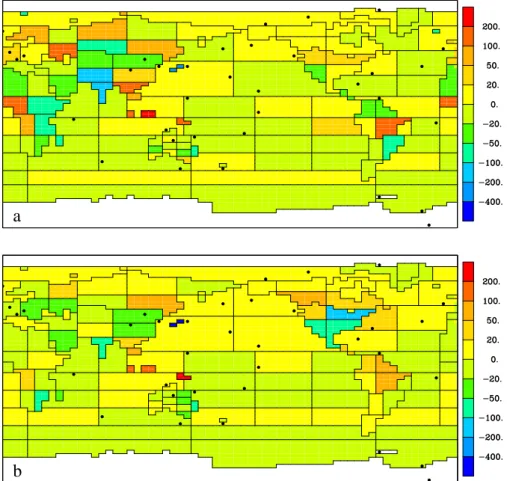
Fig. 1. Bias in 1982–1997 mean source for (a) the 4HR inversion and (b) the MON inversion. The bias is defined as the difference between
the estimated sources and the correct sources. The units are gC m−2yr−1. The dots indicate the locations of the sampling sites and the lines indicate the region boundaries.
nl/∼houwelng/TRANSCOM/t3l3 protocol.htm). The prior sources account for estimates of land-use change. They are typically small and positive for tropical land regions and small and negative for northern mid-latitude land re-gions and zero elsewhere (including all ocean rere-gions). The TransCom3, level 3 source uncertainties were taken as dou-ble those used for the TransCom3 annual mean inversion (Gurney et al., 2002). These are defined for 11 land and 11 ocean regions. These uncertainties are allocated to our smaller regions by weighting the source variance by net pri-mary production for land regions and area for ocean re-gions. The mean uncertainty for land regions is around 500 gC m−2yr−1 and around 80 gC m−2yr−1 for ocean re-gions. The prior sources and uncertainties are listed for all regions in the supplementary material, Table 1.
2.1 Sequential synthesis inversion
The method we use is somewhat similar to the sequential up-dating described by Rodgers (2000) (sec 5.8.1.3). Our moti-vation is not the usual computational cost but the size of the arrays involved in solving for the whole period at once. In
contrast to Rodgers (2000), we do not introduce one datum at a time but rather one year of data is introduced at each step. The inversion is run in two-year overlapping segments. The steps involved for the case presented here are as follows.
1. For 1981 the inversion is run for a single year and sources are estimated for 1981.
2. The 1982 data are introduced to the inversion, which is run for 1981 and 1982. The 1981 source estimates and uncertainties from step 1 (ignoring any covariance be-tween sources) are used as the prior estimates for 1981 while the 1982 prior estimates are the TransCom3-based ones. The 1982 CO2data improve the source estimates
for 1981 (because, for example, January concentrations will contain information about December sources). The 1981 data are not used in this second step because data should not be used twice in an estimation.
3. The process is repeated, advancing one year at a time. Each time the two-year inversion uses the source esti-mates and uncertainties from the previous inversion to provide the prior information for the first year while in-troducing new concentration data for the second year.
R. M. Law: Interannual CO2inversion method 479
a
b
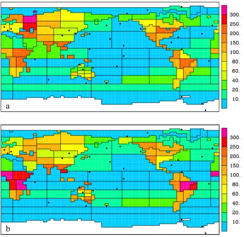
Fig. 2. Root mean square bias in the mean seasonal cycle of sources between the (a) 4HR and (b) MON inversion results and the correct
sources. The units are gC m−2yr−1.
The omission of covariances in step 2 simplifies both the algorithm and computation. An investigation of the predicted covariance matrix from step 2 showed no influence of prior covariances on the results from the first year for any month earlier than December. The predicted covariance from step 1 for December showed that 99.3% of correlations had magni-tude less than 0.35. Thus it appears that the diagonal approx-imation of the covariance matrix is a good one.
Comparing the sequential method to a five year inversion (two years spin-up, three years data, 1993–1995), showed that the first step of the sequential method gives very similar sources for all but the final month of the inversion period. For example, the average RMS bias for December 1994 sources from the sequential inversion compared to the five-year in-version was 0.16 GtC yr−1compared to RMS biases of less
than 0.04 GtC yr−1 for the other months of 1994. Largest biases occurred for regions that are more distant from the data. However, these source estimates are corrected in the next step of the inversion, when the new year of data is in-troduced. The December 1994 RMS bias is reduced from 0.16 to 0.06 GtC yr−1 and the November value from 0.04 to 0.03 GtC yr−1. The source uncertainties show a similar
pattern with the December uncertainty needing both steps of the sequential method to give an uncertainty comparable to that from the five-year inversion. Hence, to reconstruct a full timeseries of fluxes from the two-year overlapping inver-sions, it is best to retain the source estimates from November year 1 to October year 2. For the final year of the inversion (1997), the year 2 November and December estimates are used to complete the calendar year (with the understanding that these estimates may be less reliable). The good compar-ison between the sequential and five-year inversion supports the diagonal approximation of the covariance matrix in the sequential method.
2.2 Data
The synthetic data are created from a forward model run with interannually-varying ocean, biosphere and fossil fluxes. Monthly fluxes are used with linear interpolation between months. The diurnal cycle of fluxes is neglected here. The fossil sources are taken from Andres et al. (1996). The spatial distribution of the fluxes is fixed in time but the magnitude increases to match global emission estimates (Marland and Boden, 1997). The ocean fluxes are from an ocean general
480 R. M. Law: Interannual CO2inversion method
a
b
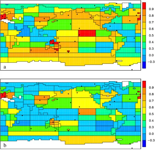
Fig. 3. Correlation between estimated and correct residual sources for (a) 4HR and (b) MON inversions.
circulation model (Le Qu´er´e et al., 2000, 2003) and the bio-sphere fluxes are from a model driven by observed tempera-ture, precipitation and solar radiation (Friedlingstein et al., 1995). These fluxes have plausible interannual variations and provide an appropriate test for the inversion method. Note that they will not necessarily sum to the known global CO2 flux inferred from atmospheric concentrations.
Invert-ing synthetic data does provide a simpler test than the real world since we assume that we can perfectly model atmo-spheric transport but this allows for a cleaner evaluation of the inversion method.
The model simulation was sampled four hourly at 35 lo-cations (Fig. 1). These lolo-cations are all places where CO2
is currently sampled (except the central Australian point), though mostly with flask measurements rather than contin-uously. The higher density of data and smaller regions for Australia provide a best-case example of how the inversion would perform if a larger network of sites was available. The four-hourly data are averaged to give monthly concen-trations, to provide the input data for a standard inversion of monthly-mean data to compare with the inversion of four-hourly data.
A data uncertainty is applied to each concentration record and is chosen to incorporate representation error (the
inabil-ity of a model to perfectly represent the data) as well as mea-surement precision. We derived the uncertainties for the four-hourly data from those applied to the monthly mean data, which were the prescribed uncertainties for the TransCom3, level 3 experiment. While here we average all four-hourly data to produce the monthly mean, in reality most monthly mean data are generated from approximately four, weekly, samples. Since data uncertainty should scale by the square root of the number of samples, we double the monthly mean uncertainties to use with the four-hourly data. This gives data uncertainties that range from 0.66 ppm for South Pole to 9.30 ppm for Hungary. A full list of data uncertainties is given in the supplementary material, Table 2.
2.3 Experiments
The sequential synthesis inversion described above is per-formed using four-hourly data from the full data set of 35 sites. The 1981 source estimates are discarded (as unreli-able) and the analysis is performed for 1982–1997. We refer to this inversion as “4HR”. For comparison, an inversion us-ing monthly mean data is also performed. The same prior sources and uncertainties are used as the four-hourly data case. We refer to this inversion as “MON”.
R. M. Law: Interannual CO2inversion method 481
a
b
Fig. 4. Difference in standard deviation of estimated and correct residual sources for (a) 4HR and (b) MON inversions. The units are
gC m−2yr−1.
In a second set of experiments, the sequential synthesis inversion is repeated but the response functions at the data locations are truncated after 3, 6, and 9 months. The remain-ing months of the year-long response are manufactured us-ing an exponential decay. Fits to the full 12 month responses at a test site showed that a decay time of approximately 90 days was appropriate, which is substantially shorter than in-terhemispheric mixing times.
2.4 Measures of inversion quality
To compare the 4HR inversion with the MON inversion, the source estimates for each region are decomposed into the 1982–1997 mean, a mean seasonal cycle (by averaging the same month in all years and subtracting the 1982–1997 mean), and the residual. The residual represents interan-nual variations (IAV). Both inversions are compared with the known, input sources. For the mean seasonal cycle, we cal-culate a root mean square bias:
RMSB= v u u t 1 12 12 X n=1 (Sn−Fn)2 (1)
where Snis the seasonal component of the estimated source for month n and Fn is the seasonal component of the cor-rect source for month n. For the interannual component of the sources, we calculate the correlation between the es-timated and correct residual fluxes. The correlation mea-sures the similarity in temporal structure between these two fluxes without reference to their magnitude. As a measure of the magnitude of the interannual variability, we compare the standard deviation of the estimated and correct residual fluxes.
To assess the inversions using shorter responses (3, 6, 9 months), the source estimates are compared to those using 12 month responses. The root mean square bias for each region is calculated from the full monthly sources for 1982–1997.
3 Results and discussion
3.1 Comparison of 4HR and MON inversions
Figure 1 shows the bias in 1982–1997 source estimates for the two inversions. In both cases the 1982–1997 mean source is estimated to within ±20 gC m−2yr−1 for all, but
482 R. M. Law: Interannual CO2inversion method
a
b
c
d
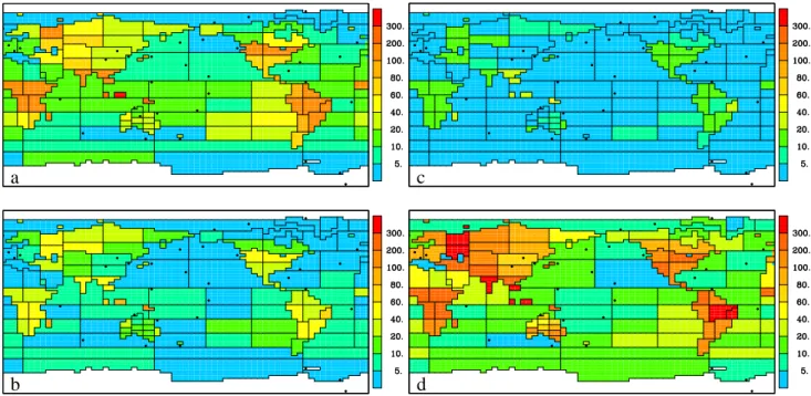
Fig. 5. Root mean square difference in source between inversion results using (a) 3 month, (b) 6 month and (c) 9 month responses and
that using 12 month responses. To give an indication of the significance of the difference, the root mean square source difference between inversion results using 12 month responses and the correct sources is shown in panel (d). The units are gC m−2yr−1.
one, ocean regions. The biases for land regions are larger especially for the 4HR inversion (only 35% of land regions within ±20 gC m−2yr−1compared to 55% for the MON in-version). The larger biases tend to occur for regions without sites nearby. Most of the bias is likely to be due to the in-teraction between the poor data constraint and aggregation errors (Kaminski et al., 2001) caused by the different spatial pattern of sources within a region for the input source and for the basis functions. An incorrect spatial pattern will re-sult in a mismatch in fitting the data, which the inversion tries to correct, often by placing large sources or sinks in regions with only a weak response at that site. The aggregation bi-ases appear to be larger with the use of more frequent data (Law et al., 2002).
Figure 2 shows the RMS bias for the estimated mean sea-sonal cycle. For both inversions, there are larger biases for land regions than ocean regions, as expected since the sea-sonal cycle of land fluxes is larger than that of the ocean fluxes. Mostly the 4HR inversion gives somewhat better re-sults than the MON inversion. This is noticeable for southern land regions. The 4HR inversion almost always gives better results for regions that include, or are close by, a measuring site.
Figure 3 shows the correlation and Fig. 4 the difference in standard deviation between the interannual component of the estimated and correct sources. The correlations are larger for more regions in the 4HR inversion than the MON inversion. For example, in the 4HR inversion 53 regions show
correla-tions greater than 0.6 whereas in the MON inversion only 17 regions show correlations of that magnitude. The magnitude of the variability is also better, for these regions with large correlation, in the 4HR case; the difference in standard devi-ation is less than ±20 gC m−2yr−1for 72% of regions with correlation greater than 0.6 for 4HR compared to only 41% for MON. Mostly the magnitude of the variability is too small in the MON case, particularly for land regions, whereas in the 4HR case southern Africa and South America tend to show variability that is too small while in Eurasia and South-East Asia the variability is too large. In the 4HR case, the lowest correlations are for the tropical Indian ocean and the tropical and south Atlantic ocean, even with data at Seychelles (5◦S, 55◦E) and Ascension (8◦S, 14◦W). In the next section we investigate whether the larger variability on land is misallo-cated to the nearby ocean regions and “swamps” the ocean variability.
3.2 Other inversion tests with four-hourly data
The sensitivity of the inversion to the prior source uncertain-ties has been tested by running a case in which the prior source uncertainty is halved. Overall there are only small differences in the source estimates. The differences in the 1982–1997 mean tend to move the solution closer to the cor-rect sources for most regions. Changes in correlation are small with positive differences for about 60% of the regions. The magnitude of the interannual variability is reduced as expected, given the smaller prior source uncertainty. This
R. M. Law: Interannual CO2inversion method 483
improves the variability for those regions that were originally overestimated (Eurasia) but degrades it for those regions that were underestimated (southern Africa and South America).
To investigate the idea that ocean variability is masked by misallocation of land variability, an inversion is per-formed using synthetic data generated from the ocean fluxes only. For ocean regions, there are small improvements in the 1982–1997 mean results and the mean seasonal cycle. IAV correlations for the ocean regions improve markedly; 25 re-gions show correlations greater than 0.6 compared to only 15 previously and 17 of these are above 0.7 compared to only seven previously. The improvements are especially notice-able in the tropical and northern Atlantic and in the tropical Indian ocean (though the correlations remain low around the Bay of Bengal). There is little change in the magnitude of in-terannual variability. This result supports the idea that ocean IAV is masked by misallocated land IAV. It is not clear what the solution to this is, given that in the real world, we cannot measure “ocean-only” concentrations. A higher density of observing sites may minimise the problem.
3.3 Comparison of inversions with shorter responses Figure 5 shows the RMS difference in total source (calcu-lated across all months from 1982–1997) between the 4HR inversion using 12 month responses and inversions using 3, 6 and 9 month responses. Also shown is the RMS difference between the 4HR inversion and the correct sources. This pro-vides a benchmark against which to assess the differences due to changing the response length. As expected the dif-ferences from the 12 month case decrease as the response length increases. The largest RMS differences occur mostly for the land regions that do not have a site nearby: central Eurasia, tropical Africa, South America and tropical Asia. In the 3 month case, the largest differences are comparable to the differences between the 12 month sources and the correct sources. This suggests that using a response length of only 3 months may compromise the inversion results. In the 6 month case, the RMS differences are smaller than the bench-mark. Thus, if computational resources are limited, it would appear that 6 month responses could be used and an adequate inversion still obtained.
4 Conclusions
The inversion results presented here have shown that contin-uous CO2measurements could be used to estimate sources
with relatively small changes to the current inversion tech-niques used with monthly mean data. The size of the inver-sion can be made feasible by running sequentially in two-year overlapping time intervals. The cpu time required to generate the response functions can be reduced by only run-ning the atmospheric transport model for six months and ap-proximating the rest of the response with an exponential
de-cay. In the tests performed here, better results were gener-ally achieved using the continuous data than using monthly data, especially for interannual variations. Aggregation bi-ases continue to be seen in the multi-year mean results, sug-gesting the need for smaller regions in the inversion set-up and more data. Future work is required to repeat these tests using a transport model capable of using analysed (and con-sequently interannually varying) winds. The plan would then be to run some test inversions using real continuous data from around twenty sites worldwide, supplemented with data from flask networks.
Acknowledgements. C. Trudinger and P. Rayner provided useful
comments on the manuscript.
Edited by: P. Kasibhatla
References
Andres, R. J., Marland, G., Fung, I., and Matthews, E.: A 1◦×1◦ distribution of carbon dioxide emissions from fossil fuel con-sumption and cement manufacture, 1950–1990, Global Bio-geochem. Cycles, 10, 419–429, 1996.
Biraud, S., Ciais, P., Ramonet, M., Simmonds, P., Kazan, V., Mon-fray, P., O’Doherty, S., Spain, G., and Jennings, S. G.: Quantifi-cation of carbon dioxide, methane, nitrous oxide and chloroform emissions over Ireland from atmospheric observations at Mace Head, Tellus, 54B, 41–60, 2002.
Friedlingstein, P., Fung, I., Holland, E., John, J., Brasseur, G., Er-ickson, D., and Schimel, D.: On the contribution of CO2
fertil-ization to the missing biospheric sink, Global Biogeochem. Cy-cles, 9, 541–556, 1995.
Gurney, K. R., Law, R. M., Denning, A. S., Rayner, P. J., Baker, D., Bousquet, P., Bruhwiler, L., Chen, Y.-H., Ciais, P., Fan, S., Fung, I. Y., Gloor, M., Heimann, M., Higuchi, K., John, J., Maki, T., Maksyutov, S., Masarie, K., Peylin, P., Prather, M., Pak, B. C., Randerson, J., Sarmiento, J., Taguchi, S., Takahashi, T., and Yuen, C.-W.: Towards robust regional estimates of CO2
sources and sinks using atmospheric transport models, Nature, 415, 626–630, 2002.
Kaminski, T., Rayner, P. J., Heimann, M., and Enting, I. G.: On ag-gregation errors in atmospheric transport inversions, J. Geophys. Res., 106, 4703–4715, 2001.
Law, R. M. and Rayner, P. J., Impacts of seasonal covariance on CO2inversions, Global Biogeochem. Cycles, 13, 845–856,
1999.
Law, R. M., Rayner, P. J., Steele, L. P., and Enting, I. G.: Using high temporal frequency data for CO2 inversions, Global
Bio-geochem. Cycles, 16, 1053, doi:10.1029/2001GB001593, 2002. Law, R. M., Rayner, P. J., Steele, L. P., and Enting, I. G.: Data and modelling requirements for CO2 inversions using
high frequency data, Tellus, 55B, 512–521, doi:10.1034/j.1600-0560.2003.0029.x, 2003.
Le Qu´er´e, C., Orr, J. C., Monfray, P., Aumont, O., and Madec, G.: Interannual variability of the oceanic sink of CO2 from
1979 through 1997, Global Biogeochem. Cycles, 14, 1247–1265, 2000.
484 R. M. Law: Interannual CO2inversion method
Le Qu´er´e, C., Aumont, O., Bopp, L., Bousquet, P., Ciais, P., Francey, R., Heimann, M., Keeling, C. D., Keeling, R. F., Kheshgi, H., Peylin, P., Piper, S. C., Prentice, I. C., and Rayner, P. J.: Two decades of ocean CO2 sink and variability, Tellus,
55B, 649–656, doi:10.1034/j.1600-0560.2003.00043.x, 2003. Marland, G. and Boden, T.: Estimates of global, regional, and
na-tional annual CO2-emissions from fossil-fuel burning, hydraulic
cement production, and gas flaring: 1950–1994, NDP-030R7, Carbon Dioxide Information Analysis Center, Oak Ridge Na-tional Laboratory, 1997.
Rayner, P. J., Enting, I. G., Francey, R. J., and Langenfelds, R. L.: Reconstructing the recent carbon cycle from atmospheric CO2, δ13C and O2/N2observations, Tellus, 51B, 213–232, 1999. Rodgers, C. D.: Inverse methods for atmospheric sounding: Theory
and practice, World Scientific Publishing Co. Pte. Ltd. 2000. Wang, Y.-P. and McGregor, J. L.: Estimating regional terrestrial
carbon fluxes for the Australian continent using a multiple-constraint approach. II. The atmospheric multiple-constraint, Tellus, 55B, 290–304, doi:10.1034/j.1600-0560.2003.00030.x, 2003.