HAL Id: hal-00328008
https://hal.archives-ouvertes.fr/hal-00328008v2
Submitted on 14 Feb 2007
HAL is a multi-disciplinary open access
archive for the deposit and dissemination of
sci-entific research documents, whether they are
pub-lished or not. The documents may come from
teaching and research institutions in France or
abroad, or from public or private research centers.
L’archive ouverte pluridisciplinaire HAL, est
destinée au dépôt et à la diffusion de documents
scientifiques de niveau recherche, publiés ou non,
émanant des établissements d’enseignement et de
recherche français ou étrangers, des laboratoires
publics ou privés.
shipping on Atmospheric Chemistry and Climate in
2000 and 2030
V. Eyring, D. S. Stevenson, A. Lauer, F. J. Dentener, T. Butler, W. J.
Collins, K. Ellingsen, M. Gauss, D. A. Hauglustaine, I.S.A. Isaksen, et al.
To cite this version:
V. Eyring, D. S. Stevenson, A. Lauer, F. J. Dentener, T. Butler, et al.. Multi-model simulations of
the impact of international shipping on Atmospheric Chemistry and Climate in 2000 and 2030.
Atmo-spheric Chemistry and Physics, European Geosciences Union, 2007, 7 (3), pp.757-780.
�10.5194/ACP-7-757-2007�. �hal-00328008v2�
www.atmos-chem-phys.net/7/757/2007/ © Author(s) 2007. This work is licensed under a Creative Commons License.
Chemistry
and Physics
Multi-model simulations of the impact of international shipping on
Atmospheric Chemistry and Climate in 2000 and 2030
V. Eyring1, D. S. Stevenson2, A. Lauer1, F. J. Dentener3, T. Butler4, W. J. Collins5, K. Ellingsen6, M. Gauss6, D. A. Hauglustaine7, I. S. A. Isaksen6, M. G. Lawrence4, A. Richter8, J. M. Rodriguez9, M. Sanderson5,
S. E. Strahan9, K. Sudo10, S. Szopa7, T. P. C. van Noije11, and O. Wild10,*
1DLR, Institut f¨ur Physik der Atmosph¨are, Oberpfaffenhofen, Germany
2University of Edinburgh, School of GeoSciences, Edinburgh, UK
3European Commission, Joint Research Centre, Institute for Environment and Sustainability, Ispra, Italy
4Max Planck Institute for Chemistry, Mainz, Germany
5Met Office, Exeter, UK
6University of Oslo, Department of Geosciences, Oslo, Norway
7Laboratoire des Sciences du Climat et de l’Environnement, Gif-sur-Yvette, France
8University of Bremen, Institute for Environmental Physics, Bremen, Germany
9Goddard Earth Science & Technology Center (GEST), Maryland, Washington, DC, USA
10Frontier Research Center for Global Change, JAMSTEC, Yokohama, Japan
11Royal Netherlands Meteorological Institute (KNMI), Atmospheric Composition Research, De Bilt, the Netherlands
*now at: University of Cambridge, Centre for Atmospheric Science, Cambridge, UK
Received: 1 August 2006 – Published in Atmos. Chem. Phys. Discuss.: 12 September 2006 Revised: 25 January 2007 – Accepted: 1 February 2007 – Published: 14 February 2007
Abstract. The global impact of shipping on atmospheric
chemistry and radiative forcing, as well as the associated uncertainties, have been quantified using an ensemble of ten state-of-the-art atmospheric chemistry models and a pre-defined set of emission data. The analysis is performed for present-day conditions (year 2000) and for two future ship emission scenarios. In one scenario ship emissions stabi-lize at 2000 levels; in the other ship emissions increase with a constant annual growth rate of 2.2% up to 2030 (termed the “Constant Growth Scenario” (CGS)). Most other an-thropogenic emissions follow the IPCC (Intergovernmental Panel on Climate Change) SRES (Special Report on Emis-sion Scenarios) A2 scenario, while biomass burning and nat-ural emissions remain at year 2000 levels. An intercompari-son of the model results with observations over the Northern
Hemisphere (25◦–60◦N) oceanic regions in the lower
tro-posphere showed that the models are capable to reproduce
ozone (O3) and nitrogen oxides (NOx=NO+NO2) reasonably
well, whereas sulphur dioxide (SO2) in the marine
bound-ary layer is significantly underestimated. The most
pro-nounced changes in annual mean tropospheric NO2and
sul-phate columns are simulated over the Baltic and North Seas. Other significant changes occur over the North Atlantic, the Gulf of Mexico and along the main shipping lane from Eu-rope to Asia, across the Red and Arabian Seas. Maximum
Correspondence to: V. Eyring
(Veronika.Eyring@dlr.de)
contributions from shipping to annual mean near-surface O3
are found over the North Atlantic (5–6 ppbv in 2000; up
to 8 ppbv in 2030). Ship contributions to tropospheric O3
columns over the North Atlantic and Indian Oceans reach 1
DU in 2000 and up to 1.8 DU in 2030. Tropospheric O3
forcings due to shipping are 9.8±2.0 mW/m2 in 2000 and
13.6±2.3 mW/m2in 2030. Whilst increasing O3, ship NOx
simultaneously enhances hydroxyl radicals over the remote ocean, reducing the global methane lifetime by 0.13 yr in 2000, and by up to 0.17 yr in 2030, introducing a negative
radiative forcing. The models show future increases in NOx
and O3 burden which scale almost linearly with increases
in NOxemission totals. Increasing emissions from shipping
would significantly counteract the benefits derived from
re-ducing SO2emissions from all other anthropogenic sources
under the A2 scenario over the continents, for example in Europe. Globally, shipping contributes 3% to increases in
O3 burden between 2000 and 2030, and 4.5% to increases
in sulphate under A2/CGS. However, if future ground based emissions follow a more stringent scenario, the relative im-portance of ship emissions will increase. Inter-model
dif-ferences in the simulated O3 contributions from ships are
significantly smaller than estimated uncertainties stemming from the ship emission inventory, mainly the ship emission totals, the distribution of the emissions over the globe, and the neglect of ship plume dispersion.
1 Introduction
Seagoing ships emit exhaust gases and particles into the marine boundary layer contributing significantly to the to-tal budget of anthropogenic emissions from the transporta-tion sector (e.g. Olivier et al., 2001; Eyring et al., 2005a).
Emissions of nitrogen oxides (NOx=NO+NO2) from
ship-ping lead to tropospheric ozone (O3) formation and perturb
the hydroxyl radical (OH) field, and hence the lifetime of
methane (CH4). These changes affect the Earth’s radiation
budget as O3and CH4are greenhouse gases. Evidence for
the importance of ship emissions comes from satellite obser-vations from GOME (Beirle et al., 2004) and SCIAMACHY
(Richter et al., 2004) that show enhanced tropospheric NO2
columns along the major international shipping routes in the Red Sea and over the Indian Ocean. A number of atmo-spheric model studies quantifying the impact of ship emis-sions on the chemical composition of the atmosphere and on climate have been published in recent years. All these studies used a global fuel consumption of about 160 million metric tons (Mt, or Tg) per year derived from energy statistics (Cor-bett and Fischbeck, 1997; Cor(Cor-bett et al., 1999; Olivier et al., 2001; Endresen et al., 2003). However, there is an ongoing discussion on the present-day value, as recent estimates of the fuel consumption calculated with an activity-based ap-proach indicate higher fuel consumption of around 280 Mt (Corbett and K¨ohler, 2003; Eyring et al., 2005a), suggesting that previous model studies may have significantly underes-timated emissions. Despite this, these models tend to
over-estimate oceanic NOx over parts of the North Atlantic and
the Pacific (Lawrence and Crutzen, 1999; Kasibahtla et al., 2000; Davis et al., 2001; Endresen et al., 2003). One possi-bility to reduce this discrepancy might be to account for ship plume dispersion in global models (Kasibhatla et al., 2000; Davis et al., 2001; Song et al., 2003; von Glasow et al., 2003;
Chen et al., 2005). In ship plumes the lifetime of NOxis
sig-nificantly reduced compared to the background and NOx in
the plume is rapidly oxidised. Some NOx is therefore lost
at scales smaller than the typical grid size of global mod-els (100–500 km). These sub-grid-scale processes have to be parameterised in global models, e.g., by the use of effective emission indices depending on the meteorology and back-ground conditions. However, there is no clear consensus on the effective global emissions from ships. In this study we use relatively low global emission estimates and neglect ship plume chemistry.
In addition to NOx, shipping contributes significantly to
global sulphur dioxide (SO2) emissions as the average
sul-phur content of the fuel burned in marine diesel engines of 2.4% is high compared to other transport sectors (EPA,
2002). In large areas of the Northern Hemisphere SO2
emis-sions from ships are comparable to biogenic dimethyl sul-phide (DMS) emissions, which are the main natural source of sulphur over the oceans (Corbett et al., 1999; Capaldo et al., 1999; Derwent et al., 2005). The main oxidation
pro-cesses for SO2 are believed to be either via OH in the gas
phase or in the liquid phase via O3or H2O2in cloud droplets
(Langner and Rohde, 1991). As SO2is primarily controlled
by aqueous processes, it is expected that SO2is largely
inde-pendent of enhanced OH in the plume (Davis et al., 2001). In
addition to sulphate particles resulting from SO2emissions,
ships also release black carbon (BC) and particulate organic matter (POM). The increase in sulphate, BC and POM con-centrations has a direct and indirect effect on climate. The di-rect effect results from enhanced scattering of solar radiation (Haywood and Shine, 1995). The indirect effect of particles from shipping results from changes in the microphysical, op-tical and radiative properties of low marine clouds (Scorer, 1987; Capaldo et al., 1999, Durkee et al., 2000; Schreier et al., 2006).
The numbers of ships in the world merchant fleet has in-creased by 35% over the past 50 years, accompanied by a sig-nificant increase in emission totals (Eyring et al., 2005a). At the end of the year 2001 it consisted of around 90 000 ocean-going ships of 100 gross tons (GT) and above (Lloyd’s, 2002). Shipping is currently one of the less regulated sources of anthropogenic emissions with a high reduction potential through technological improvements, alternative fuels and ship modifications. Emission scenario calculations up to the year 2050 show that if no control measures are taken beyond existing International Maritime Organization (IMO)
regula-tions (IMO, 1998), NOx emissions might increase with an
annual growth rate of 1.7% between 2000 and 2030 and up to a value of present day global road transport by 2050 (38.8 Tg (NO2)/yr) (Eyring et al., 2005b). If the sulphur content
re-mains at present day levels a doubling of ship SO2emissions
can be expected. However, given the air quality issue of
ship-ping emissions, further emission reductions of total NOxand
SO2 emissions are likely. Using aggressive NOx emission
reduction technologies, a significant decrease up to 85% of
today’s NOxemissions could be reached through
technolog-ical improvements by 2050, in spite of a growing fleet. A summary of current national and international maritime reg-ulations is given in Eyring et al. (2005b).
Currently there is a large uncertainty about the overall impact of emissions from international shipping which can
be explored using global atmospheric models. The first
key question addressed in this study is how NOx and SO2
emissions from international shipping might influence
at-mospheric chemistry, in particular tropospheric O3and
sul-phate, in the next three decades, if these emissions increase
unabated. To address this, impacts of NOx and SO2
emis-sions from international shipping are assessed with the help of an ensemble of state-of-the-art global atmospheric
chem-istry models. The second major issue is to examine the
range of results given by the individual models compared to the ensemble mean to estimate the uncertainties intro-duced by different modelling approaches. The participat-ing models have also been evaluated and used in accompa-nying studies (e.g. Stevenson et al., 2006; Dentener et al.,
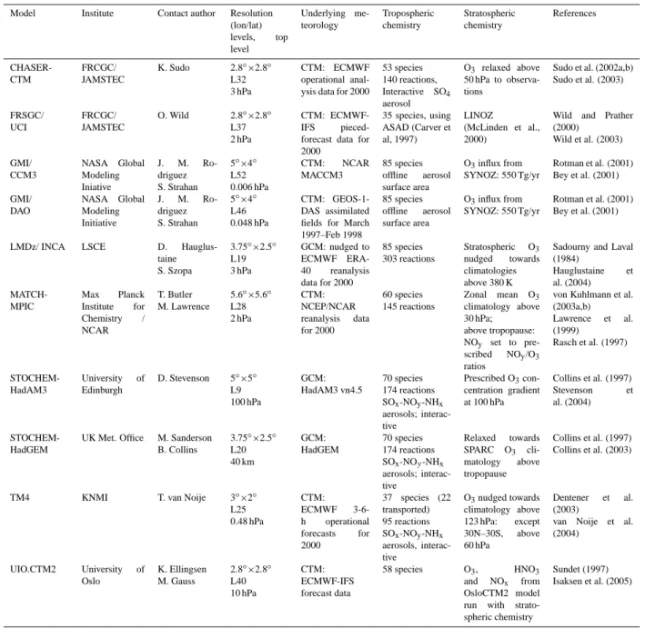
Table 1. Participating models. The models are listed alphabetically by name. The horizontal resolution is given in degrees latitude × longitude.
Model Institute Contact author Resolution (lon/lat) levels, top level Underlying me-teorology Tropospheric chemistry Stratospheric chemistry References CHASER-CTM FRCGC/ JAMSTEC K. Sudo 2.8◦×2.8◦ L32 3 hPa CTM: ECMWF operational anal-ysis data for 2000
53 species 140 reactions, Interactive SO4 aerosol O3 relaxed above 50 hPa to observa-tions
Sudo et al. (2002a,b) Sudo et al. (2003) FRSGC/ UCI FRCGC/ JAMSTEC O. Wild 2.8◦×2.8◦ L37 2 hPa CTM: ECMWF-IFS pieced-forecast data for 2000 35 species, using ASAD (Carver et al, 1997) LINOZ (McLinden et al., 2000)
Wild and Prather (2000) Wild et al. (2003) GMI/ CCM3 NASA Global Modeling Iniative J. M. Ro-driguez S. Strahan 5◦×4◦ L52 0.006 hPa CTM: NCAR MACCM3 85 species offline aerosol surface area O3influx from SYNOZ: 550 Tg/yr Rotman et al. (2001) Bey et al. (2001) GMI/ DAO NASA Global Modeling Initiative J. M. Ro-driguez S. Strahan 5◦×4◦ L46 0.048 hPa CTM: GEOS-1-DAS assimilated fields for March 1997–Feb 1998 85 species offline aerosol surface area O3influx from SYNOZ: 550 Tg/yr Rotman et al. (2001) Bey et al. (2001)
LMDz/ INCA LSCE D. Hauglus-taine S. Szopa 3.75◦×2.5◦ L19 3 hPa GCM: nudged to ECMWF ERA-40 reanalysis data for 2000 85 species 303 reactions Stratospheric O3 nudged towards climatologies above 380 K
Sadourny and Laval (1984) Hauglustaine et al. (2004) MATCH-MPIC Max Planck Institute for Chemistry / NCAR T. Butler M. Lawrence 5.6◦×5.6◦ L28 2 hPa CTM: NCEP/NCAR reanalysis data for 2000 60 species 145 reactions Zonal mean O3 climatology above 30 hPa; above tropopause: NOy set to pre-scribed NOy/O3 ratios
von Kuhlmann et al. (2003a,b) Lawrence et al. (1999) Rasch et al. (1997) STOCHEM-HadAM3 University of Edinburgh D. Stevenson 5◦×5◦ L9 100 hPa GCM: HadAM3 vn4.5 70 species 174 reactions SOx-NOy-NHx aerosols; interac-tive Prescribed O3 con-centration gradient at 100 hPa Collins et al. (1997) Stevenson et al. (2004) STOCHEM-HadGEM
UK Met. Office M. Sanderson B. Collins 3.75◦×2.5◦ L20 40 km GCM: HadGEM 70 species 174 reactions SOx-NOy-NHx aerosols; interac-tive Relaxed towards SPARC O3 cli-matology above tropopause Collins et al. (1997) Collins et al. (2003)
TM4 KNMI T. van Noije 3◦×2◦
L25 0.48 hPa CTM: ECMWF 3-6-h operational forecasts for 2000 37 species (22 transported) 95 reactions SOx-NOy-NHx aerosols, interac-tive O3nudged towards climatology above 123 hPa: except 30N–30S, above 60 hPa Dentener et al. (2003)
van Noije et al. (2004) UIO.CTM2 University of Oslo K. Ellingsen M. Gauss 2.8◦×2.8◦ L40 10 hPa CTM: ECMWF-IFS forecast data 58 species O3, HNO3 and NOx from OsloCTM2 model run with strato-spheric chemistry
Sundet (1997) Isaksen et al. (2005)
2006a,b; Shindell et al., 2006, van Noije et al., 2006) as part of the European Union project ACCENT (Atmospheric Composition Change: the European NeTwork of excellence; http://www.accent-network.org).
The models and model simulations, together with the method to analyse the results are described in Sect. 2. The
models’ ability to simulate O3, NOx and SO2 over the
re-mote ocean is evaluated in Sect. 3.1. Large-scale chemistry
effects on NO2and O3distributions due to NOxemissions
from ships are discussed in Sect. 3.2 for present-day
condi-tions and in Sect. 3.3 for 2030, while impacts of SO2
emis-sions from ships on sulphate distributions are discussed in Sect. 3.4. In Sect. 3.5 radiative forcings (RFs) from
tro-pospheric O3 calculated with the help of an offline
radia-tion scheme are summarised and RFs due to carbon
diox-ide (CO2), CH4, and sulphate are roughly estimated.
Sec-tion 4 discusses the impact of volatile organic compounds (VOC) and carbon monoxide (CO) emissions from ships and possible uncertainties in the presented results mainly stem-ming from the emission inventory itself, the neglect of plume
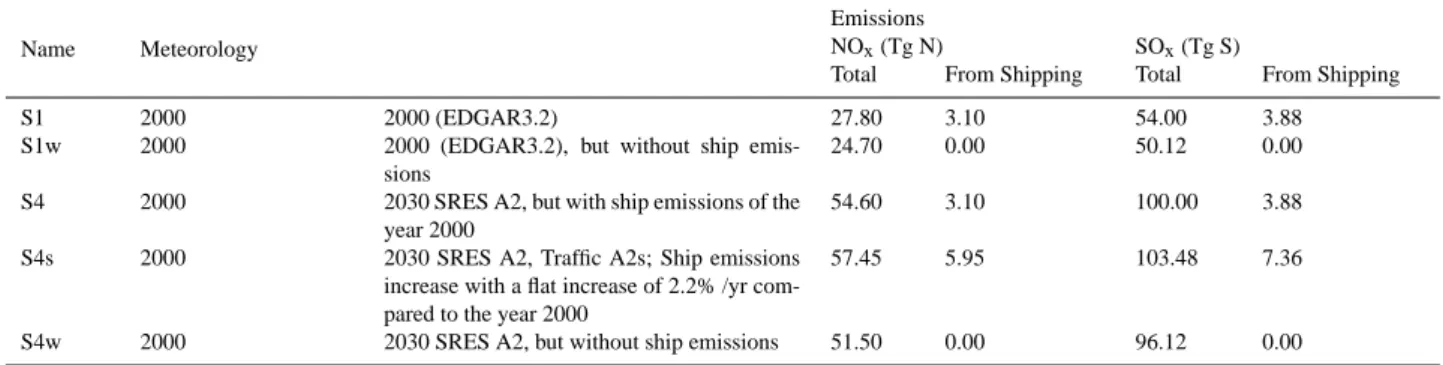
Table 2. Specified global annual anthropogenic (not including biomass burning emissions) surface emission totals for each scenario.
Name Meteorology
Emissions
NOx(Tg N) SOx(Tg S)
Total From Shipping Total From Shipping
S1 2000 2000 (EDGAR3.2) 27.80 3.10 54.00 3.88
S1w 2000 2000 (EDGAR3.2), but without ship
emis-sions
24.70 0.00 50.12 0.00
S4 2000 2030 SRES A2, but with ship emissions of the
year 2000
54.60 3.10 100.00 3.88
S4s 2000 2030 SRES A2, Traffic A2s; Ship emissions
increase with a flat increase of 2.2% /yr com-pared to the year 2000
57.45 5.95 103.48 7.36
S4w 2000 2030 SRES A2, but without ship emissions 51.50 0.00 96.12 0.00
chemistry and assumptions in the future scenarios for back-ground as well as ship emissions. Section 5 closes with a summary and conclusions.
2 Models and model simulations
2.1 Participating Models
Ten global atmospheric chemistry models have participated in this model inter-comparison. Seven of the ten models are Chemistry-Transport Models (CTMs) driven by meteoro-logical assimilation fields and three models are atmospheric General Circulation Models (GCMs). Two of the GCMs are driven with the dynamical fields calculated by the GCM in climatological mode, but the fully coupled mode (interaction between changes in radiatively active gases and radiation) has been switched off in the simulations of this study. The other GCM runs in nudged mode, where winds and temper-ature fields are assimilated towards meteorological analyses. Therefore, changes in the chemical fields do not influence the radiation and hence the meteorology in any of the model simulations used here, and for a given model each scenario is driven by identical meteorology. The main characteristics of the ten models are summarised in Table 1 and the models are described in detail in the cited literature.
The horizontal resolution ranges from 5.6◦×5.6◦
(MATCH-MPIC) to 2.8◦×2.8◦ (CHASER-CTM,
FRSGC/UCI, UIO.CTM2) and 3◦×2◦ (TM4). The
vertical resolution varies in terms of number of vertical layers and upper boundary and ranges from 9 layers with a model top at 100 hPa (STOCHEM-HadAM3) to 52 layers with a model top at 0.006 hPa (GMI/CCM3).
All models use detailed tropospheric chemistry schemes even though notable differences exist between the models, e.g. in the hydrocarbon chemistry. Of the ten models, four included the tropospheric sulphur cycle (CHASER-CTM, STOCHEM-HadAM3, STOCHEM-HadGEM, and TM4). These models include anthropogenic and natural sulphur sources, and account for oxidation in the gas phase by OH,
and in the aqueous phase (in cloud droplets) by H2O2 and
O3. Sulphate aerosol is predominantly removed by
wet-deposition processes. Models also differ in the parameter-isation of sub-grid scale convection, the representation of cloud and hydrological processes, dry and wet deposition, and boundary layer mixing and a variety of different advec-tion schemes are used.
Differences in the main characteristics as listed above will
lead to differences in the modelled response to NOxand SO2
emissions from shipping, even if near-identical forcings (e.g., sea surface temperatures, natural and anthropogenic emis-sions, and meteorology) are used. A more detailed discussion of the sources of differences between the models is included in Stevenson et al. (2006).
2.2 Model Simulations
Two of the five simulations that have been defined as part of the wider PHOTOCOMP-ACCENT-IPCC study have been used in this work: a year 2000 base case (S1) and a year 2030 emissions case (S4) following the IPCC (Intergovern-mental Panel on Climate Change) SRES (Special Report on Emission Scenarios) A2 scenario (IPCC, 2000). Full details on the emissions used in the S1 and S4 simulations are sum-marised in Stevenson et al. (2006) and only the key aspects for this study are given here. All models used the same an-thropogenic and biomass burning emissions, but variable
nat-ural emissions. For example, for NOx, natural sources from
soils and lightning differ between the models, but this has
little impact over the oceans. For SO2, natural sources from
volcanoes and oceanic DMS differ. The latter has some
im-pact on absolute values of SO2over the oceans, but little
im-pact on changes due to ships. The differences in natural emis-sions are not thought to be a major source of inter-model dif-ferences in the results presented here. To retain consistency with all other emissions, ship emissions in the year 2000 (S1) are based on the EDGAR3.2 dataset (Olivier et al., 2001) at
a spatial resolution of 1◦latitude×1◦longitude. The global
distribution of ship emissions in EDGAR3.2 is based on the world’s main shipping routes and traffic intensities (Times
180°W 180°W 120°W 120°W 60°W 60°W 0° 0° 60°E 60°E 120°E 120°E 180° 180° 60°S 60°S 0° 0° 60°N 60°N 2000 180°W 180°W 120°W 120°W 60°W 60°W 0° 0° 60°E 60°E 120°E 120°E 180° 180° 60°S 60°S 0° 0° 60°N 60°N 2030 0.02 0.05 0.10 0.20 0.50 1.00 2.00 5.00 g(N)/(m2 yr)
Fig. 1. Annual surface NOxemissions including industry and power generation, traffic, domestic heating, and biomass burning (average
1997–2002 (van der Werf, 2004) in g(N)/(m2yr). The left plot shows the emissions used as input for the model experiment S1 (year 2000,
38.0 Tg(N)/yr total), the right plot the emissions for experiment S4s (year 2030, 67.6 Tg(N)/yr total).
Books, 1992; IMO, 1992). EDGAR3.2 includes data for 1995, which have been scaled to 2000 values assuming a
growth rate of 1.5%/yr, resulting in annual NOx and SO2
emissions of 3.10 Tg(N) and 3.88 Tg(S), respectively, sim-ilar to the emission totals published by Corbett et al. (1999). Table 2 summarises the global annual anthropogenic surface
emission and ship emission totals for NOx and SO2. In
the 2000 simulation (S1), ship emissions account for about 11.2% of all anthropogenic surface nitrogen oxide emissions and for about 7.2% of all anthropogenic sulphur emissions. Other emissions from ships such as CO, particulate matter,
CH4and VOC were not included in this inventory and were
therefore not considered in the reference simulations. The ef-fect of CO and VOC emissions from ships is quantified with the help of sensitivity simulations carried out with a single model (MATCH-MPIC) in Sect. 4.1.2.
As noted in Stevenson et al. (2006) in the S4 simulation emissions from ships were included at year 2000 levels by mistake. All other anthropogenic sources (except biomass burning emissions, which remain fixed at year 2000 levels) vary according to A2 broadly representing a pessimistic fu-ture situation. The simulation S4 is used here to assess the impact of ship emissions under different background levels. An additional model simulation for 2030 (S4s) has been de-signed to assess the impact of shipping if emission growth re-mains unabated. Ship emissions in S4s are based on a “Con-stant Growth Scenario” (CGS) in which emission factors are unchanged and emissions increase with an annual growth rate of 2.2% between 2000 and 2030. In the S4s scenario
emissions from shipping increase to 5.95 Tg(N) for NOxand
7.36 Tg(S) for SO2in 2030. As an example, the global
dis-tributions of surface NOxemissions for the years 2000 (S1)
and 2030 (S4s) are displayed in Fig. 1. Vessel traffic distribu-tions are assumed to stay the same for all model simuladistribu-tions presented here.
To assess the impact of ship emissions on chemistry and
climate in 2000 and 2030, two sensitivity simulations have been defined that use identical conditions to S1 or S4/S4s except that ship emissions are excluded. The year 2000 and 2030 experiments without ship emissions are denoted as S1w and S4w.
All 2030 model experiments (S4, S4s and S4w) are driven by the same meteorological data as the 2000 simulations (S1 and S1w). Global methane mixing ratios have been specified across the model domain (1760 ppbv in 2000 and 2163 ppbv in 2030) to save time spinning up the models and to help con-strain the results (for details see Stevenson et al., 2006). Nine of the ten models performed single year simulations with spin-ups of at least 3 months and one model (STOCHEM-HadGEM) performed a four year simulation. For the multi-annual simulations the results have been averaged over all four years to reduce the effects of inter-annual variability.
2.3 Model Analyses
Each model provided output for 3-D monthly mean NOx,
O3and sulphate mixing ratios as well as the mass of each
grid-box on the native model grid for all five simulations. As models used a variety of vertical co-ordinate systems and resolutions, the output has been converted to the same com-mon vertical grid as used in Stevenson et al. (2006). Model results are interpolated to the 19 hybrid (sigma-pressure) lev-els of the Met Office HadAM3 model where up to 14 of these levels span the troposphere. Results were also
inter-polated to a common horizontal resolution of 5◦×5◦. To
calculate the ensemble mean on the common grid the sim-ulated fields have been masked at the chemical tropopause
(O3=150 ppbv) similar to the method applied in Stevenson
et al. (2006). For the 2000 simulations (S1 and S1w) we
ap-ply a consistent mask by using the O3 field from the S1w
simulation for each model and all species. For the 2030
sim-ulations (S4, S4s, and S4w) the S4w O3field is used to mask
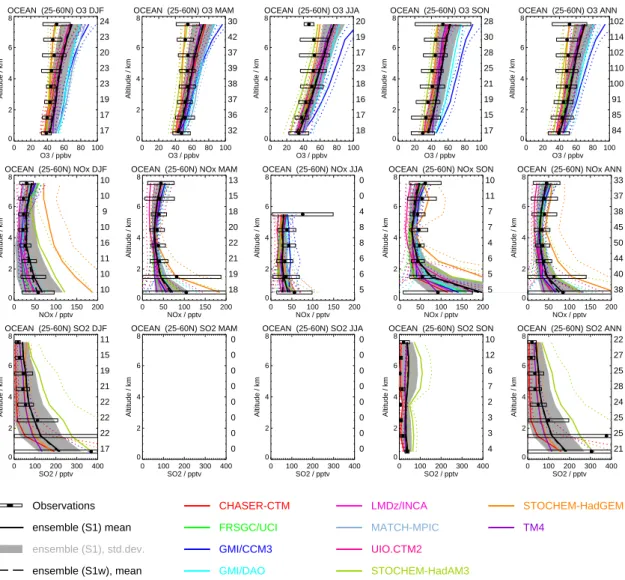
OCEAN (25-60N) O3 DJF 0 20 40 60 80 100 O3 / ppbv 0 2 4 6 8 Altitude / km 17 17 19 23 23 20 23 24 OCEAN (25-60N) O3 MAM 0 20 40 60 80 100 O3 / ppbv 0 2 4 6 8 Altitude / km 32 36 37 38 39 37 42 30 OCEAN (25-60N) O3 JJA 0 20 40 60 80 100 O3 / ppbv 0 2 4 6 8 Altitude / km 18 17 16 18 23 17 19 20 OCEAN (25-60N) O3 SON 0 20 40 60 80 100 O3 / ppbv 0 2 4 6 8 Altitude / km 17 15 19 21 25 28 30 28 OCEAN (25-60N) O3 ANN 0 20 40 60 80 100 O3 / ppbv 0 2 4 6 8 Altitude / km 84 85 91 100 110 102 114 102 OCEAN (25-60N) NOx DJF 0 50 100 150 200 NOx / pptv 0 2 4 6 8 Altitude / km 10 10 11 16 10 9 10 10
OCEAN (25-60N) NOx MAM
0 50 100 150 200 NOx / pptv 0 2 4 6 8 Altitude / km 18 19 21 22 20 18 15 13
OCEAN (25-60N) NOx JJA
0 50 100 150 200 NOx / pptv 0 2 4 6 8 Altitude / km 5 6 6 8 8 4 0 0
OCEAN (25-60N) NOx SON
0 50 100 150 200 NOx / pptv 0 2 4 6 8 Altitude / km 5 5 6 4 7 7 11 10
OCEAN (25-60N) NOx ANN
0 50 100 150 200 NOx / pptv 0 2 4 6 8 Altitude / km 38 40 44 50 45 38 37 33 OCEAN (25-60N) SO2 DJF 0 100 200 300 400 SO2 / pptv 0 2 4 6 8 Altitude / km 17 22 22 22 21 19 15 11
OCEAN (25-60N) SO2 MAM
0 100 200 300 400 SO2 / pptv 0 2 4 6 8 Altitude / km 0 0 0 0 0 0 0 0
OCEAN (25-60N) SO2 JJA
0 100 200 300 400 SO2 / pptv 0 2 4 6 8 Altitude / km 0 0 0 0 0 0 0 0
OCEAN (25-60N) SO2 SON
0 100 200 300 400 SO2 / pptv 0 2 4 6 8 Altitude / km 4 3 3 2 7 6 12 10
OCEAN (25-60N) SO2 ANN
0 100 200 300 400 SO2 / pptv 0 2 4 6 8 Altitude / km 21 25 25 24 28 25 27 22 Observations
__
ensemble (S1) mean ensemble (S1), std.dev._ _
ensemble (S1w), mean__
CHASER-CTM__
FRSGC/UCI__
GMI/CCM3__
GMI/DAO__
LMDz/INCA__
MATCH-MPIC__
UIO.CTM2__
STOCHEM-HadAM3__
STOCHEM-HadGEM__
TM4Fig. 2. Seasonal and annual means of O3(upper row, ppbv), NOx(middle row, pptv) and SO2(lower row, pptv) for the Northern Hemisphere
(25◦–60◦N) oceanic regions obtained from a compilation of observations (Emmons et al., 2000 plus updates) and calculated by the models
(S1 simulation). The mean values of the individual models are shown with solid coloured lines and the standard deviation with dotted coloured lines. The ensemble mean (all models) is drawn as dashed black line for the S1w simulation and as solid black line for the S1 simulation, the intermodel standard deviation for S1 as grey shaded areas, and the observations as filled black circles (mean) and white rectangles (standard deviation).
model results were masked in the same way (O3=150 ppbv)
but summed on their native grids, to avoid the introduction of errors associated with the interpolation (Sect. 3.3.2). The
impact of ship emissions on NOx, O3and sulphate
distribu-tions is assessed by calculating the difference between the reference simulation (S1 for 2000; S4 or S4s for 2030) and the ensemble mean of the no-ships scenario (S1w for 2000; S4w for 2030). For the calculation of instantaneous
tropo-spheric O3forcings the differences in O3fields between
sen-sitivity and reference simulations on the common grid were used (Sect. 3.5).
3 Results
3.1 Comparison of model results with observations
The models have been evaluated in accompanying
stud-ies. For example, O3fields have been compared to
ozone-sonde measurements (Stevenson et al., 2006), NO2columns
have been compared to three state-of-the-art retrievals from measurements of the Global Ozone Monitoring Experiment (GOME) (van Noije et al., 2006), CO has been compared to near-global observations from the MOPITT instrument and local surface measurements (Shindell et al., 2006), deposi-tion budgets have been compared to nearly all informadeposi-tion on wet and dry deposition available worldwide (Dentener
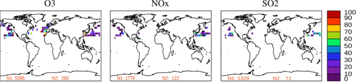
O3 NOx SO2 N1: 5395 N2: 260 N1: 1776 N2: 122 0 10 20 30 40 50 60 70 80 90 100 N1: 1329 N2: 71
Fig. 3. Geographical distribution of the number of observations in the Emmons et al. (2000) plus updates data set for O3, NOx, and SO2
in the Northern Hemisphere (25◦–60◦N) oceanic regions in the altitude range 0–3 km. N1 gives the total number of individual observations
and N2 the total number of 5◦×5◦grid boxes that include at least one observation.
et al., 2006b), and finally modelled surface O3 fields have
been compared to observations from various measurement sites (Dentener et al., 2006a). In all these studies, the en-semble mean was among the best when comparing to mea-surements. In this study we build on the model evaluation work listed above as well as on the individual evaluation of the models and make the assumption that the models produce reasonable simulations of the key chemical species. We use the ensemble mean to assess large-scale chemistry effects re-sulting from ship emissions for the present day and in the future.
In addition to the above mentioned studies, we evaluate
here the models’ ability to simulate O3, NOx and SO2 in
the lower troposphere (<3 km) as well as tropospheric NO2
columns over the ocean by comparing the results from the S1 present-day reference simulations of the individual mod-els to aircraft measurements (Emmons et al., 2000; Singh et al., 2006) and to satellite data from SCIAMACHY (Richter et al., 2004).
Tropospheric data from a number of aircraft campaigns
have been gridded onto a 5◦ longitude by 5◦ latitude grid
by Emmons et al. (2000), with additional data from more re-cent campaigns (see http://gctm.acd.ucar.edu/data), up to and including TRACE-P in 2001 (we subsequently refer to this data as “Emmons et al. (2000) plus updates”). We compare
data over the Northern Hemisphere (25◦–60◦N) oceanic
re-gions in Fig. 2. Most models reproduce the observed annual
and seasonal O3 means in the lower troposphere (<3 km).
Two models (GMI/CCM3 and GMI/DAO) simulate O3
val-ues larger than observed in autumn and winter, and
MATCH-MPIC overestimates observed O3 in winter. The oceanic
25◦–60◦N means in observations and models shown in Fig. 2
are averages over only those grid boxes that include obser-vations for the particular species (see Fig. 3). To compare model results with observations in the Pacific and Atlantic, we use data collected during the INTEX-NA campaign in July/August 2004 in addition (see http://www-air.larc.nasa. gov/; Singh et al., 2006). The good agreement between
mod-elled and observed O3in July holds for both the Pacific and
the Atlantic (Fig. 4).
In winter and autumn, the two STOCHEM models, both
using the same chemistry scheme, simulate the highest NOx
values among all models (Fig. 2). An additional analysis
showed that in these models in these seasons, high NOx
plumes from land-based anthropogenic sources were extend-ing sufficiently far out to sea to affect the nearest oceanic data comparison points. In addition, the treatment of
hetero-geneous NOxloss in the STOCHEM models is very simple,
and may be leading to unrealistically long NOxlifetimes in
winter and autumn. For all other models the simulated NOx
and NO2(not shown) lies within one standard deviation (1σ )
of the observational mean in all seasons with values above the observational mean in autumn and below in all other sea-sons as well as in the annual mean (Fig. 2). Nearly all
ob-servations for NOx over the Northern Hemisphere oceanic
regions below 3 km in the Emmons et al. (2000) plus up-dates data set are made over the Pacific (Fig. 3). Compared to
the INTEX-NA campaign, the simulated NO2lies within 1σ
of the observational mean over the Atlantic and the Pacific (Fig. 4). This overall reasonable agreement between models
and observations for NOxand NO2differs from the findings
of Kasibhatla et al. (2000) and Davis et al. (2001), who
found that their models overpredicted NOx in the Atlantic
and Pacific marine boundary layer. These authors used sim-ilar ship emissions, but compared with somewhat different observational data. Kasibhatla et al. (2000) used NARE
cam-paign data from the North Atlantic (37◦–50◦N; 35◦–50◦W)
in September 1997 and Davis et al. (2001) used data from five campaigns over the North Pacific.
SO2in the four models that included a sulphur cycle
gen-erally lie within 1σ of the observations in Fig. 2, but there is little data outside the winter season, and the standard devia-tions in the marine boundary layer are large, making it diffi-cult to assess the models. One of the models (STOCHEM-HadAM3) is consistently high, particularly in the free tropo-sphere – this is probably related to the relatively large
mag-nitude and elevated source of volcanic SO2 in this model.
Standard deviations are smaller in the summertime INTEX-NA data set over the Pacific (Fig. 4). All models significantly
underestimate observed SO2in July, in agreement with
pre-vious findings (Davis et al., 2001).
1 2
Fig. 4. Observations from the INTEX-NA campaign from 1 July to 15 August 2004 (Singh et al., 2006) compared to the July mean of the
S1 model simulations for O3(left), NO2(middle), and SO2(right) over the Atlantic (upper row, 60◦W–36◦W, 28◦N–53◦N) and the Pacific
(lower row, 140◦W–126◦W, 34◦N–45◦N). The ensemble mean for S1 (all models) is shown as solid black line and for S1w as dashed black
line. The intermodel standard deviation for the S1 ensemble mean is shown as grey shaded areas, and the observations as filled black circles (mean) and black error bars (standard deviation).
that ship plume chemistry may partly explain the
discrep-ancy between observed and simulated NOx. While the
ne-glect of ship plume chemistry in global models might con-tribute to differences between observations and models, we show here that the selection of data the models are com-pared to is also very important: if we reduce the Emmons et al. (2000) plus updates and the INTEX-NA data set and
only compare the model results for NOxwith the data used in
Davis et al. (2001) we can reproduce their results. However, if we use the entire observational data set (Fig. 2), which is more widespread and therefore more robust (up to 32 cam-paigns between 1983 and 2001, including the five Pacific
datasets, but not including the Atlantic NARE data) we find
good agreement with observed NOx. In addition, differences
in the modelled and observed NOx and SO2fields can not
be fully attributed to ship emissions. In particular, the com-parison with the Emmons et al. (2000) plus updates and the INTEX-NA data sets leads to only small differences between the S1 and the S1w ensemble mean (Figs. 2 and 4), so that the shipping signal cannot be properly evaluated. Therefore,
it remains unclear whether the underestimation of SO2 in
the marine boundary layer in the models is due to the ship emission inventory or due to the underestimation of another source (e.g. DMS), overestimation of a sink (e.g. oxidation),
30°E 30°E 45°E 45°E 60°E 60°E 75°E 75°E 90°E 90°E 105°E 105°E 120°E 120°E 0° 0° 10°N 10°N 20°N 20°N 30°N 30°N 40°N 40°N SCIAMACHY 0.0 2.5 5.0 7.5 10.0 12.5 15.0 0.5°x0.5° tropospheric NO2 (VC) in 1014 molec/cm2 30°E 30°E 45°E 45°E 60°E 60°E 75°E 75°E 90°E 90°E 105°E 105°E 120°E 120°E 0° 0° 10°N 10°N 20°N 20°N 30°N 30°N 40°N 40°N 30°E 30°E 45°E 45°E 60°E 60°E 75°E 75°E 90°E 90°E 105°E 105°E 120°E 120°E 0° 0° 10°N 10°N 20°N 20°N 30°N 30°N 40°N 40°N
model ensemble mean, S1
30°E 30°E 45°E 45°E 60°E 60°E 75°E 75°E 90°E 90°E 105°E 105°E 120°E 120°E 0° 0° 10°N 10°N 20°N 20°N 30°N 30°N 40°N 40°N
Fig. 5. NOxsignature of shipping in the Indian Ocean (5◦S to 40◦N and 25◦E to 125◦E). Left: Tropospheric NO2columns derived from
SCIAMACHY data from August 2002 to April 2004 (Richter et al., 2004). Right: Ensemble mean NO2tropospheric columns at 10.30 local
time for 2000. The ensemble mean comprises 8 out of the 10 models. Individual model results and SCIAMACHY data were interpolated to
a common grid (0.5◦×0.5◦).
errors associated with simulating specific events (e.g. hor-izontal/vertical transport and mixing), or a combination of several factors. More measurements are needed before final conclusions on the quality of the models to simulate the ship emission response can be made (see also Sect. 5).
Another approach to evaluate the shipping response in models is the use of satellite data. Recently, enhanced
tro-pospheric NO2 columns have been observed over the Red
Sea and along the main shipping lane to the southern tip of India, to Indonesia and north towards China and Japan (Beirle et al., 2004; Richter et al., 2004). Here we
inter-compare the tropospheric NO2columns derived from
SCIA-MACHY nadir measurements from August 2002 to April 2004 (Richter et al., 2004) to the models’ ensemble mean in 2000 (S1 simulation). The ensemble mean in Fig. 5 consists
of the eight models that provided tropospheric NO2columns
at 10:30 a.m. local time, which is close to the overpass time of the ERS-2 satellite. The two STOCHEM models provided output only as 24 h mean, and are not included. To com-pare the model data to the satellite measurements, individual model results and SCIAMACHY data were interpolated to a
common grid (0.5◦×0.5◦). The models simulate similar
tro-pospheric NO2columns over the remote ocean as observed
by SCIAMACHY and also reproduce the overall pattern of the geographical distribution reasonably well. However, al-though the shipping signal is clearly visible in the satellite data it is not resolved by the models, because the
intercom-parison of modelled and observed NO2columns is
compli-cated by several factors. First of all, the spatial resolution
of the SCIAMACHY measurements (30×60 km2) is much
higher than that of the global models (typically 5◦×5◦)
lead-ing to higher NO2values in the localized plumes from ship
emissions. Secondly, in the particular scene shown in Fig. 5, shipping routes are rather close to land. Given the low resolu-tion of the models, the grid boxes close to the coast are
dom-inated by NOxemissions from land sources which are much
stronger than emissions from shipping. Thus, the shipping signal cannot be identified in the coarse resolution model data in this region. From this point of view, an intercom-parison over the remote ocean (e.g. over the Atlantic) with satellite data far away from any land source would be prefer-able. However, up to now, no statistically significant satel-lite data on ship emissions are available for remote oceans. This is mainly due to the distributed nature of the emissions which leads to dilution and makes it difficult to distinguish the shipping signal from the effect of long-range transport from the US towards Europe. Increasing ship emission in the future should make detection possible, in particular if data from an instrument with good spatial coverage such as OMI or GOME-2 is used in combination with model calculations of the contribution of long range transport. However, unam-biguous identification and quantification will always be more difficult than in the special case between India and Indonesia with its unique emission pattern.
3.2 Large-scale chemistry effects of NOxship emissions in
2000
To examine the range of results given by the individual mod-els compared to the ensemble mean, Fig. 6 shows differences
in annually averaged zonal mean O3versus height between
the 2000 base case simulation (S1) and the model simula-tion without shipping (S1w) for each model and the ensem-ble mean. Standard deviations are shown in addition in-dicating regions of large intermodel variability. All mod-els show the maximum contributions from ships in zonal
annual mean near-surface O3 in northern mid-latitudes
be-tween 10◦N and 55◦N, where most of the global ship
emis-sions are released into the atmosphere (see Fig. 1). A rapid
decrease of the impact on O3 distributions with height is
simulated. There are notable differences in the magnitude of the response to ship emissions between the individual models which can be attributed to differences in the main
-0.1 0 0.1 0.2 0.3 0.4 0.5 0.6 0.7 0.8 0.9 1 1.1 1.2 1.3 1.4 1.5 1.6 1.7 1.8 1.9 90S 60S 30S 0 30N 60N 90N 1.0 0.9 0.8 0.7 0.6 0.5 0.4 0.3 0.2
0.1 (a) S1-S1w CHASER-CTM AZM O3
Hybrid vertical level
-0.1 0 0.1 0.2 0.3 0.4 0.5 0.6 0.7 0.8 0.9 1 1.1 1.2 1.3 1.4 1.5 1.6 1.7 1.8 1.9 90S 60S 30S 0 30N 60N 90N 1.0 0.9 0.8 0.7 0.6 0.5 0.4 0.3 0.2 0.1 (b) S1-S1w FRSGC/UCI AZM O3
Hybrid vertical level
-0.1 0 0.1 0.2 0.3 0.4 0.5 0.6 0.7 0.8 0.9 1 1.1 1.2 1.3 1.4 1.5 1.6 1.7 1.8 1.9 90S 60S 30S 0 30N 60N 90N 1.0 0.9 0.8 0.7 0.6 0.5 0.4 0.3 0.2 0.1 (c) S1-S1w GMI/CCM3 AZM O3
Hybrid vertical level
-0.1 0 0.1 0.2 0.3 0.4 0.5 0.6 0.7 0.8 0.9 1 1.1 1.2 1.3 1.4 1.5 1.6 1.7 1.8 1.9 90S 60S 30S 0 30N 60N 90N 1.0 0.9 0.8 0.7 0.6 0.5 0.4 0.3 0.2 0.1 (d) S1-S1w GMI/DAO AZM O3
Hybrid vertical level
-0.1 0 0.1 0.2 0.3 0.4 0.5 0.6 0.7 0.8 0.9 1 1.1 1.2 1.3 1.4 1.5 1.6 1.7 1.8 1.9 90S 60S 30S 0 30N 60N 90N 1.0 0.9 0.8 0.7 0.6 0.5 0.4 0.3 0.2
0.1 (e) S1-S1w LMDZ/INCA AZM O3
Hybrid vertical level
-0.1 0 0.1 0.2 0.3 0.4 0.5 0.6 0.7 0.8 0.9 1 1.1 1.2 1.3 1.4 1.5 1.6 1.7 1.8 1.9 90S 60S 30S 0 30N 60N 90N 1.0 0.9 0.8 0.7 0.6 0.5 0.4 0.3 0.2 0.1 (f) S1-S1w MATCH-MPIC AZM O3
Hybrid vertical level
-0.1 0 0.1 0.2 0.3 0.4 0.5 0.6 0.7 0.8 0.9 1 1.1 1.2 1.3 1.4 1.5 1.6 1.7 1.8 1.9 90S 60S 30S 0 30N 60N 90N 1.0 0.9 0.8 0.7 0.6 0.5 0.4 0.3 0.2 0.1 (g) S1-S1w STOCHEM_HadAM3 AZM O3
Hybrid vertical level
-0.1 0 0.1 0.2 0.3 0.4 0.5 0.6 0.7 0.8 0.9 1 1.1 1.2 1.3 1.4 1.5 1.6 1.7 1.8 1.9 90S 60S 30S 0 30N 60N 90N 1.0 0.9 0.8 0.7 0.6 0.5 0.4 0.3 0.2 0.1 (h) S1-S1w STOCHEM_HadGEM AZM O3
Hybrid vertical level
-0.1 0 0.1 0.2 0.3 0.4 0.5 0.6 0.7 0.8 0.9 1 1.1 1.2 1.3 1.4 1.5 1.6 1.7 1.8 1.9 90S 60S 30S 0 30N 60N 90N 1.0 0.9 0.8 0.7 0.6 0.5 0.4 0.3 0.2 0.1 (i) S1-S1w TM4 AZM O3
Hybrid vertical level
-0.1 0 0.1 0.2 0.3 0.4 0.5 0.6 0.7 0.8 0.9 1 1.1 1.2 1.3 1.4 1.5 1.6 1.7 1.8 1.9 90S 60S 30S 0 30N 60N 90N 1.0 0.9 0.8 0.7 0.6 0.5 0.4 0.3 0.2 0.1 (j) S1-S1w UIO.CTM2 AZM O3
Hybrid vertical level
-0.1 0 0.1 0.2 0.3 0.4 0.5 0.6 0.7 0.8 0.9 1 1.1 1.2 1.3 1.4 1.5 1.6 1.7 1.8 1.9 90S 60S 30S 0 30N 60N 90N 1.0 0.9 0.8 0.7 0.6 0.5 0.4 0.3 0.2 0.1
(k) S1-S1w Ensemble Mean AZM O3 / ppbv
Hybrid vertical level
0 0.02 0.04 0.06 0.08 0.1 0.12 0.14 0.16 0.18 0.2 0.22 0.24 0.26 0.28 0.3 0.32 0.34 0.36 0.38 0.4 90S 60S 30S 0 30N 60N 90N 1.0 0.9 0.8 0.7 0.6 0.5 0.4 0.3 0.2 0.1
(l) S1-S1w Standard Deviation AZM O3 / ppbv
Fig. 6. Modelled zonal annual mean O3change (ppbv) between case S1 (year 2000) and S1w (year 2000 without ship emissions): (a–j)
individual models (k) ensemble mean (all 10 models) and (l) intermodel standard deviations. Individual model results were interpolated to a
common grid (5◦×5◦×19 levels) and masked at the chemical tropopause (O3=150 ppbv).
characteristics of the models (see Sect. 2.1). The two
mod-els that show the strongest response of O3to ship emissions
are the UIO.CTM2 and the STOCHEM-HadAM3 models. The models with the weakest response are the LMDz/INCA-CTM and the TM4 models. Previous studies reported that the
production of O3depends on the resolution of the model with
models having higher resolution simulating less O3
produc-tion than those with a coarser resoluproduc-tion (e.g. Esler, 2003; Wild and Prather, 2006). However, there are large differ-ences in the responses of the UIO.CTM2, CHASER and FRSGC/UCI models, all running at the highest resolution
used here (2.8◦×2.8◦), while the MATCH-MPIC model
run-ning at the coarsest horizontal resolution (5.6◦×5.6◦) has a
low O3response. It is therefore clear that factors other than
resolution play an important role in explaining the differ-ences (see Sect. 2.1). The ensemble mean shows the largest
increase in near-surface zonal mean O3 due to ships of up
to 1.3 ppbv in northern mid-latitudes with intermodel dif-ferences around 20% (Fig. 6k,l). In the free troposphere at latitudes further north changes still reach 1 ppbv with
in-termodel differences of around 0.16 ppbv (16%). In the
Southern Hemisphere no significant changes in zonal mean
O3distribution are simulated by all models. We conclude
that the range of results given by the individual models
in-dicates uncertainties of the presented ensemble means of the order of 20% near the surface and slightly lower in the free troposphere. The high standard deviations in the tropical tropopause layer are caused by a single model (CHASER). The main conclusions in the subsequent sections are based on the models’ ensemble mean.
Due to the short lifetime of NO2 in the boundary layer,
near-surface changes in NO2due to ship emissions (S1-S1w)
follow closely the main shipping routes, but the dispersion is a few hundred kilometres, which is partly due to coarse resolutions of the models, but also real transport (Fig. 7). Maximum changes of 2.3 ppbv are found over the Baltic Sea in both months. In the English Channel and along the west
coast of Europe (from Ireland to Morocco) NO2changes are
also significant (around 0.5 ppbv). Enhanced NO2levels up
to 0.2 ppbv are also simulated over large areas of the At-lantic and e.g. in the Red Sea and along the main shipping lane to the southern tip of India, to Indonesia and north to-wards China and Japan as well as in the Gulf of Mexico. In
July NO2changes over the Baltic and over the Atlantic are
smaller than in January and cover a smaller area, as the
life-time of NOxin the summer months is shorter due to higher
chemical activity. Relative changes in NO2strongly depend
Fig. 7. Modelled ensemble mean near-surface NO2and O3change between case S1 (year 2000) and S1w (year 2000 without ship emissions)
in January (left) and July (right). (a–b): absolute changes in near-surface NO2; (c–d): relative changes in near-surface NO2; (e–f) absolute
changes in near-surface O3; (g–h): relative changes in near-surface O3.
though absolute NO2changes over the Baltic and the North
Sea are large, relative changes are less pronounced because
of high background NO2levels. The largest relative changes
of up to 80% in January and 96% in July are found over the remote Atlantic and along the major shipping lanes, where
background levels are small and NOxemissions from ships
are the dominant source (see Fig. 1).
Substantial differences are simulated between the
near-surface January and July ensemble mean O3 changes
de-spite the fact that there are no seasonal variations in the ship emission inventory (Fig. 7, lower panels). The reason for
the difference is that during winter additional NOxemissions
from shipping can lead to O3titration in the highly polluted
regions over the continents, whereas in summer the
addi-tional NOx leads to O3 production. O3 concentrations in
January show a decrease of around 1 ppbv with maximum decreases of up to 2.8 ppbv over the Baltic. The changes in July over this region are rather small but positive. The
largest increases in January are found southward of 30◦N,
where the available solar radiation is sufficient for O3
pro-duction to outweigh direct removal of NO. Most pronounced increases of 3.3 ppbv are simulated over the Indian Ocean and along the main shipping lane west of the coast of
South-ern Africa. The simulated large decrease in O3over a large
area in Europe in winter, which has not been reported in e.g. the Endresen et al. (2003) study, might be due to high vessel traffic densities in particular over the Baltic Sea in the inven-tory used here. Vessel traffic densities derived from differ-ent sources such as AMVER (Automated Mutual-assistance Vessel Rescue system) or the Purple Finder (PF) data set (available at http://www.purplefinder.com) report fewer ob-servations there (Endresen et al., 2003), see further
discus-sion in Sect. 4.1.1. In July, the geographical pattern in O3
changes is similar to the pattern in Lawrence and Crutzen (1999) showing most pronounced changes over wide areas of the Atlantic up to 12 ppbv (approx. 35%) and over the
0 0.1 0.2 0.3 0.4 0.5 0.6 0.7 0.8 0.9 1 1.1 1.2 1.3 1.4 1.5 1.6 1.7 1.8 1.9 2 90S 60S 30S 0 30N 60N 90N 1.0 0.9 0.8 0.7 0.6 0.5 0.4 0.3 0.2 0.1
(a) S1-S1w Ensemble Mean AZM O3 / ppbv
Hybrid vertical level
-5 -2 -1 0 1 2 3 4 5 6 7 8 9 180 120W 60W 0 60E 120E 180 90S 60S 30S EQ 30N 60N 90N
(b) S1-S1w Ensemble Mean ANS O3 / ppbv
0 0.15 0.3 0.45 0.6 0.75 0.9 1.05 1.2 1.35 1.5 1.65 1.8 180 120W 60W 0 60E 120E 180 90S 60S 30S EQ 30N 60N 90N
(c) S1-S1w Ensemble Mean ATC O3 / DU
0 0.1 0.2 0.3 0.4 0.5 0.6 0.7 0.8 0.9 1 1.1 1.2 1.3 1.4 1.5 1.6 1.7 1.8 1.9 2 90S 60S 30S 0 30N 60N 90N 1.0 0.9 0.8 0.7 0.6 0.5 0.4 0.3 0.2 0.1
(d) S4-S4w Ensemble Mean AZM O3 / ppbv
Hybrid vertical level
-5 -2 -1 0 1 2 3 4 5 6 7 8 9 180 120W 60W 0 60E 120E 180 90S 60S 30S EQ 30N 60N 90N
(e) S4-S4w Ensemble Mean ANS O3 / ppbv
0 0.15 0.3 0.45 0.6 0.75 0.9 1.05 1.2 1.35 1.5 1.65 1.8 180 120W 60W 0 60E 120E 180 90S 60S 30S EQ 30N 60N 90N
(f) S4-S4w Ensemble Mean ATC O3 / DU
0 0.1 0.2 0.3 0.4 0.5 0.6 0.7 0.8 0.9 1 1.1 1.2 1.3 1.4 1.5 1.6 1.7 1.8 1.9 2 90S 60S 30S 0 30N 60N 90N 1.0 0.9 0.8 0.7 0.6 0.5 0.4 0.3 0.2 0.1
(g) S4s-S4w Ensemble Mean AZM O3 / ppbv
Hybrid vertical level -5 -2 -1 0 1 2 3 4 5 6 7 8 9 180 120W 60W 0 60E 120E 180 90S 60S 30S EQ 30N 60N 90N
(h) S4s-S4w Ensemble Mean ANS O3 / ppbv
0 0.15 0.3 0.45 0.6 0.75 0.9 1.05 1.2 1.35 1.5 1.65 1.8 180 120W 60W 0 60E 120E 180 90S 60S 30S EQ 30N 60N 90N
(i) S4s-S4w Ensemble Mean ATC O3 / DU
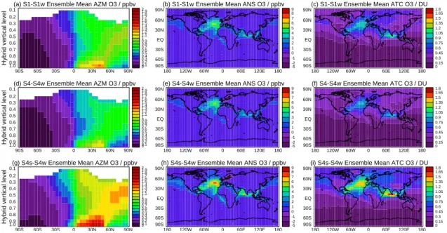
Fig. 8. Modelled ensemble mean O3change between (a–c) case S1 (year 2000) and S1w (year 2000 without ship emissions), (d–f) case S4
(year 2030) and S4w (year 2030 without ship emissions), and (g–i) case S4s (year 2030) and S4w. Figures 8a, 8d, and 8g are zonal mean
changes (ppbv), Figs. 8b, 8e, and 8h are near-surface O3changes (ppbv) and Figs. 8c, 8f, and 8i are tropospheric O3column changes (DU).
Western and Northern Pacific up to 5 ppbv (approx. 25%). Changes of the order of 5 ppbv (approx. 10%) are also sim-ulated over the Indian Ocean. The simsim-ulated changes over the Atlantic and the Indian Ocean are in good agreement with results reported in Endresen et al. (2003), but smaller over the Pacific. Differences between the two studies are likely related to the difference in vessel traffic densities (see
Sect. 4.1.1). Due to the longer lifetime of O3 compared
to NO2 in the boundary layer, O3changes are less strictly
confined to the main shipping lanes, and thus affect larger
areas. Non-linear effects of O3photochemistry are
signifi-cant. For example, over the Baltic and the North Sea, where
background NO2levels are relatively high, changes in O3are
comparatively small, whereas they are substantial over more remote areas.
3.3 Large-scale chemistry effects of NOxship emissions in
2030
3.3.1 Ozone distributions
Figure 8 shows modelled ensemble mean O3changes due to
ship emissions for the year 2000 (S1-S1w) and for two dif-ferent scenarios in 2030 (S4-S4w; S4s-S4w). As vessel traf-fic densities are the same in all model simulations the 2030 results mainly show a scaling of the 2000 results, but
non-linearity effects also play a role. O3changes versus height in
2000 (Fig. 8a) have already been discussed in Sect. 3.1. The
largest O3response is found near the surface between 10◦–
55◦N, and rapidly decreases with altitude. Keeping
sions from shipping at 2000 levels but with all other emis-sions increasing, the pattern in zonal mean changes remains the same but the impact is slightly less than in 2000 due to
lower O3production rates under the influence of higher
back-ground of NOxconcentrations (Fig. 8d; S4-S4w). Under the
S4s scenario near-surface O3changes of about 1.7 ppbv are
simulated in the zonal mean between 10◦–55◦N, and even
in the free troposphere changes in O3reach up to 1.3 ppbv
(Fig. 8g). Changes in the annual mean near-surface level reach 5.5 ppbv over the Atlantic (Fig. 8b) and increase up to 7.4 ppbv in the S4s scenario in 2030 (Fig. 8h). Over
North-ern Europe where there are high levels of NOx, the increase
in NOxfrom shipping decreases, rather than increases, O3
levels. This is due to reduction in oxidant levels as OH is
removed by the reaction NO2+ OH -> HNO3, and in winter
to direct titration of O3by NO2. The effect is stronger in the
2030 scenarios due to the increased background level of NOx
in Northern Europe, with shipping decreasing O3by 3 ppbv
in the S4s scenario.
The most pronounced changes in tropospheric O3columns
are found over the Indian Ocean (1.16 DU in 2000 and 1.72 DU in 2030), related to the higher tropopause there and to
more effective transport of O3 from the boundary into the
upper troposphere. A second peak is simulated over the At-lantic (Figs. 8c,f,i).
1
Figure 9. Global total change in annual mean tropospheric NO burden (left) and O burden 2
Fig. 9. Global total change in annual mean tropospheric NOxburden (left) and O3burden (right) due to ship emissions (S4-S4w and
S4s-S4w) in each individual model (coloured lines) and the ensemble mean (black line). Inter-model standard deviations are shown as black bars.
3.3.2 Linearities in NOx and O3 burden response to ship
emissions
Changes in annual mean NOxand O3burdens are calculated
for the two 2030 scenarios (S4-S4w; S4s-S4w) as described in Sect. 2.3 for four different regions (global mean, Atlantic Ocean, Baltic Sea, and Indian Ocean). A linear regression
is performed for the changes in NOxand O3burdens due to
shipping over the scenarios S4-S4w, S4s-S4w and the
ori-gin (zero NOxship emissions / zero changes in NOxand O3
burdens). The changes in global tropospheric NOx burden
associated with these two scenarios show a fairly linear
rela-tionship for all models (Fig. 9, left), and a doubling of NOx
emissions approximately results into a doubling of the mean
NOxburden.
For O3the correlation is also broadly linear (Fig. 9, right).
Only small saturation effects are visible as the O3burden for
the low emission scenario (3.10 Tg(N)) lies slightly above the multi-regression line whereas the one for the high emission scenario (5.95 Tg(N)) lies slightly below the multi-regression
line for all models. This is to be expected due to
non-linearities in the O3 chemistry. In contrast to the relatively
small degree of saturation computed here, Labrador et al. (2004) computed a substantial saturation effect for lightning
NOxemissions as they were increased from 0 to 20 Tg(N)/yr,
with the saturation already becoming clearly evident between 5 and 10 Tg(N)/yr. Although there are only three data points
available here (0, 3.1 and 5.95 Tg(N)/yr), there is evidence
in these results that the ship NOxeffect is only weakly
sub-ject to saturation in its current magnitude range, and that sat-uration cannot be expected to help mitigate the effects of
near-future increases. Overall, similar to NOx burdens, a
doubling in NOxship emissions results in approximately a
doubling in O3 burdens in the ensemble mean. Note that,
whereas the majority of the models (eight out of ten) show
similar response, the two STOCHEM models simulate NOx
burden changes around a factor of 3 (STOCHEM-HadAM3) or 6 (STOCHEM-HadGEM) higher than the other models, which explains the large standard deviations of the ensemble
mean NOxburden. As discussed in Sect. 3.1, this can mainly
be attributed to high NOx plumes from land-based
anthro-pogenic sources and to the long NOxlifetimes in winter and
autumn in these two models. For the annual O3burdens the
two STOCHEM models show similar results compared to all
other models, and the inter-model standard deviations for O3
are small (<15%).
Similar to the global annual burdens, eight out of the ten
models show similar response in the seasonal cycle of NOx
and O3 burden changes for the S4s-S4w scenario over the
Atlantic Ocean, the Baltic Sea, the Indian Ocean and
glob-ally (Fig. 10). As expected, the seasonal cycle in both NOx
and O3is most pronounced in the Baltic Sea (northern
1
Figure 10. Seasonal variation in tropospheric NO (left column) and O (middle column) 2
Fig. 10. Seasonal variation in tropospheric NOx(left column) and O3(middle column) burden due to shipping for the scenario S4s-S4w
in different regions: Atlantic Ocean (85◦W–5◦W; 15◦N–60◦N), Baltic Sea (10◦E–30◦E; 54◦N–66◦N), Indian Ocean (50◦E–100◦E;
0◦N–25◦N) and global.
cycle over the Indian Ocean is relatively small. Again the two STOCHEM models show significantly higher changes in
NOxburdens in winter and autumn in northern mid-latitude
regions (Atlantic and Baltic Sea). The change in ensemble
mean O3burdens reaches peak values of about 0.8 Tg over
the Atlantic in August, 0.4 Tg over the Indian Ocean in Oc-tober, and 0.04 Tg over the Baltic Sea in June. The global
change in NOxburden due to ship emissions as simulated by
the ensemble mean in the S4s scenario is enhanced by 25 Gg
in summer. The global O3burden is enhanced by about 4 Tg
with peak changes in October and smallest changes in Jan-uary.
3.4 Large-scale chemistry effects of SO2ship emissions in
2000 and 2030
A subset of four models (CHASER, STOCHEM-HadAM3, STOCHEM-HadGEM, and TM4) included the tropospheric sulphur cycle. The ensemble mean of these four models has been applied to quantify changes due to shipping in sul-phate distributions now and in the future (Fig. 11). Maxi-mum changes due to shipping in the ensemble mean zonal
mean sulphate (SO4) distribution are located in the
bound-ary layer of the northern mid-latitudes around 40◦N. These
-4 0 3 6 9 12 15 18 21 24 27 30 33 36 39 42 45 48 51 54 60 90S 60S 30S 0 30N 60N 90N 1.0 0.9 0.8 0.7 0.6 0.5 0.4 0.3 0.2
0.1 (a) S1-S1w Ensemble Mean AZM SO4 / pptv
Hybrid vertical level -90 0 30 60 90 120 150 180 210 240 270 300 330 180 120W 60W 0 60E 120E 180 90S 60S 30S EQ 30N 60N
90N (b) S1-S1w Ensemble Mean ANS SO4 / pptv
-0.15 0 0.15 0.3 0.45 0.6 0.75 0.9 1.05 1.2 1.35 1.5 1.65 180 120W 60W 0 60E 120E 180 90S 60S 30S EQ 30N 60N 90N
(c) S1-S1w Ensemble Mean ATC SO4 [mg/m2]
-4 0 3 6 9 12 15 18 21 24 27 30 33 36 39 42 45 48 51 54 60 90S 60S 30S 0 30N 60N 90N 1.0 0.9 0.8 0.7 0.6 0.5 0.4 0.3 0.2
0.1 (d) S4-S4w Ensemble Mean AZM SO4 / pptv
Hybrid vertical level -90 0 30 60 90 120 150 180 210 240 270 300 330 180 120W 60W 0 60E 120E 180 90S 60S 30S EQ 30N 60N
90N (e) S4-S4w Ensemble Mean ANS SO4 / pptv
-0.15 0 0.15 0.3 0.45 0.6 0.75 0.9 1.05 1.2 1.35 1.5 1.65 180 120W 60W 0 60E 120E 180 90S 60S 30S EQ 30N 60N 90N
(f) S4-S4w Ensemble Mean ATC SO4 [mg/m2]
-4 0 3 6 9 12 15 18 21 24 27 30 33 36 39 42 45 48 51 54 60 90S 60S 30S 0 30N 60N 90N 1.0 0.9 0.8 0.7 0.6 0.5 0.4 0.3 0.2
0.1 (g) S4s-S4w Ensemble Mean AZM SO4 / pptv
Hybrid vertical level -90 0 30 60 90 120 150 180 210 240 270 300 330 180 120W 60W 0 60E 120E 180 90S 60S 30S EQ 30N 60N
90N (h) S4s-S4w Ensemble Mean ANS SO4 / pptv
-0.15 0 0.15 0.3 0.45 0.6 0.75 0.9 1.05 1.2 1.35 1.5 1.65 180 120W 60W 0 60E 120E 180 90S 60S 30S EQ 30N 60N 90N
(i) S4s-S4w Ensemble Mean ATC SO4 [mg/m2]
Fig. 11. Modelled ensemble mean tropospheric sulphate changes between (a–c) case S1 (year 2000) and S1w (year 2000 without ship emissions), (d–f) case S4 (year 2030) and S4w (year 2030 without ship emissions), and (g-i) case S4s (year 2030) and S4w. Figures 11a, 11d, and 11g are zonal mean changes (pptv), Figs. 11b, 11e, and 11h are near-surface sulphate changes (pptv) and Figs. 11c, 11f, and 11i
are tropospheric sulphate column changes (mg/m2). Individual model results were interpolated to a common grid (5◦×5◦×19 levels) and
masked at the chemical tropopause (O3=150 ppbv). The ensemble mean comprises four models.
Table 3. O3, SO4, CO2, and CH4radiative forcings due to shipping in 2000 and 2030. The RF resulting from the indirect aerosol effect
is not included but is expected to be negative and larger in magnitude than the direct sulphate effects estimated here (Capaldo et al., 1999). Ozone forcings include inter-model standard deviations, based on the ensemble of 10 models. Other forcings are rough central estimates with larger, less well constrained uncertainties, see Sect. 3.5.
O3mW/m2 SO4(direct) mW/m2 CH4mW/m2 CO2mW/m2
2000 (S1-S1w) 9.8±2.0 –14 –14 26
2030 (S4-S4w) 7.9±1.4 –13 –13 24
2030 (S4s-S4w) 13.6±2.3 –26 –21 46
and 50 pptv in the year 2030 (S4s-S4w). With increasing
height, the changes in SO4decrease continuously to about 3–
5 pptv (2000) and 6–9 pptv (2030) in the upper troposphere. In the lowermost boundary layer over the Atlantic Ocean at the west coast of Europe and over the Baltic Sea, maximum annual sulphate changes amount to about 200 pptv in 2000 and 300 pptv in 2030. The geographical pattern shows the main shipping routes over the Atlantic Ocean between Eu-rope and North America and over the Red Sea and the Indian Ocean between the Arabian Peninsula and India. In all other
parts of the world, changes in sulphate due to SO2emissions
from shipping remain low in general. Globally, shipping con-tributes with 4.5% to sulphate increases until 2030 under the A2/CGS.
3.5 Radiative Forcing
O3distributions from all scenarios and all models were used
as input for an offline radiation scheme (Edwards and Slingo, 1996), with all other parameters held constant, broadly
repre-senting the present-day atmosphere. In the stratosphere, O3
was overwritten by a climatology, so the changes discussed here are purely tropospheric. The calculations include the radiative effects of clouds. Comparing instantaneous short-wave and long-short-wave radiative fluxes at the tropopause
be-tween scenarios yields O3radiative forcings (see Stevenson
et al. (1998) for more details on the method). In order to
make the O3forcings directly comparable to other forcings,
stratospheric temperatures, which respond on timescales of a month or so to radiative perturbations, need to be adjusted until there is no change in stratospheric heating rates, the so-called “fixed dynamical heating” approximation. Stevenson
Fig. 12. Ensemble mean for instantaneous tropospheric O3forcing (a) plus standard deviations (b) in mW/m2.
et al. (1998) found that this relaxation of stratospheric
tem-peratures resulted in a 22% reduction in the O3forcing
com-pared to the instantaneous value and we apply this as a glob-ally constant correction. Figure 12a shows maps of
multi-model ensemble mean annual mean instantaneous O3
radia-tive forcings for the 2030 high emissions case (S4s) relaradia-tive to the scenario without ships (S4w). Similar distributions were found for the other scenarios. The peak forcing
oc-curs over the Indian Ocean, the site of the largest column O3
changes (Fig. 8), but also a region with relatively high sur-face temperatures, and a high, cold tropopause. A secondary peak occurs over the Caribbean for similar reasons. Further north over the Atlantic the forcing is less, despite a
signifi-cant O3change, reflecting the smaller surface-to-tropopause
temperature contrast and increasing cloudiness.
Figure 12b shows the inter-model standard deviation, which is typically 15–25%. The ensemble mean forcings and standard deviations for the three cases (S1-S1w, S4-S4w and S4s-S4w), applying a 22% reduction to account for strato-spheric temperature adjustment, are 9.8±2.0, 7.9±1.4 and
13.6±2.3 mW/m2, respectively. The influence of ship
emis-sions on the O3forcing slightly reduces as the background
O3levels rise, but the relationship between ship NOx
emis-sions and resultant O3forcing is close to linear. Comparing
with the total O3 forcing between 2000 and 2030, as
dis-cussed in Stevenson et al. (2006), the contribution from ships
in the S4s case to the global projected tropospheric O3
forc-ing is 4%.
Ship NOx emissions also affect the radiatively active gas
methane, by increasing OH and reducing the methane life-time. Five models (CHASER-CTM, FRSGC/UCI, LMDz-INCA, STOCHEM-HadAM3 and TM4) provided methane destruction fluxes for each scenario, and these were used
to calculate whole atmosphere CH4 lifetimes, as described
in Stevenson et al. (2006). For four of the five models,
changes in lifetime between scenarios were very consistent (within 4% of each other), but STOCHEM-HadAM3 was nearly twice as sensitive, and is thus considered an outlier. Here we use ensemble mean results from the four models
to assess ship impacts on CH4lifetime. For present-day, ship
NOxshortens the CH4lifetime by 0.13 yr (1.56±0.05%)
(S1-S1w); in 2030 the same ship NOxperturbation reduces the
lifetime by 0.10 yr (1.14±0.02%) (S4-S4w), again illustrat-ing the slightly lower sensitivity when background levels are higher. Following the A2/CGS the methane lifetime is re-duced by an additional 0.07 yr (0.77±0.02%) in 2030
(S4s-S4). Ship NOxtherefore introduces a negative radiative
forc-ing by reducforc-ing the build-up of methane. We make a first-order estimate of the methane radiative forcing by linearly scaling the methane lifetime changes, assuming a feedback factor of 1.4 (IPCC, 2001) to infer a change in methane mix-ing ratio, and then calculate global mean forcmix-ing usmix-ing the
value of 0.37 W/m2ppb−1for a globally uniform methane
change (Schimel et al., 1996). Estimated methane forcings are given in Table 3.
The various contributions to the radiative forcing from
shipping also include radiative forcing due to CO2 and
sul-phate changes. The corresponding radiative forcing of CO2
is estimated from the fraction of the ship emission totals in the year 2000 (136.7 Tg(C)/yr, Endresen et al. (2003)) to the
total annual CO2emissions in 2000 (7970 Tg(C)/yr, IPCC
(2001), scenario A2). This fraction (1.7%) is used to scale
the RF resulting from all CO2 sources (1.51 W/m2, IPCC
(2001), scenario A2, ISAM reference case) linearly,
result-ing in a RF of 26 mW/m2 due to shipping. The same
ap-proach is used to estimate CO2RF for the year 2030, with
annual emissions of 14,720 Tg(C)/yr for all sources (IPCC
(2001), scenario A2) and a total CO2RF of 2.59 W/m2(IPCC
(2001), scenario A2, ISAM reference case). The emissions from shipping are assumed to increase at an annual rate of 2.2% since 2000, resulting in 262.6 Tg(C)/yr in 2030. For the simulation S4, shipping contributes with 0.9% to the total
an-nual CO2emissions, for S4s with 1.8%. This results in CO2
RF of about 24 mW/m2(S4-S4w) and 46 mW/m2(S4s-S4w)
due to shipping in 2030. However, since CO2has a long
av-erage lifetime, the time integral of ship emissions would be needed to estimate a more accurate number for RF.
Direct sulphate forcings are calculated from the change
in total SO4 burdens due to shipping. The relative change
of the SO4burdens is used to scale the total direct radiative
forcing of sulphate particles given by IPCC (2001) (scenario