Development of a wearable blood pressure monitor using adaptive calibration of peripheral pulse transit time measurements

TS INSTRUTE ,OLOGYr

2008

RIES

CALIBRATION OF PERIPHERAL PULSE TRANSIT TIME MEASUREMENTS

by

•M;iASSACHt S.EqT" DEVIN BARNETT MCCOMBIE

Bachelor of Science in Bioengineering University of California, San Diego, 2000

OF 17:.'.0H"HN

SEP

18

LIBRA

Master of Science in Mechanical Engineering Massachusetts Institute of Technology, 2004

Master of Science in Electrical Engineering and Computer Science Massachusetts Institute of Technology, 2004

SUBMITTED TO THE DEPARTMENT OF MECHANICAL ENGINEERING

IN PARTIAL FULFILLMENT OF THE REQUIREMENTS FOR THE DEGREE OF

DOCTOR OF PHILOSOPHY

AT THE

MASSACHUSETTS INSTITUTE OF TECHNOLOGY

JUNE 2008

C 2008 Massachusetts Institute of Technology. All rights reserved.

Signature of Author... ...

Certified By ...

. ...

Department of Mechanical Engineering May 19, 2008

Y H. Harry Asada

Ford Professor of Mechanical Engineering Thesis Supervisor

Accepted by... -- ....--- ...

Lallit Anand Chairman, Department Committee on Graduate Students

DEVELOPMENT OF A WEARABLE BLOOD PRESSURE MONITOR USING ADAPTIVE CALIBRATION OF PERIPHERAL PULSE TRANSIT TIME MEASUREMENTS

by

DEVIN BARNETT MCCOMBIE

Submitted to the Department of Mechanical Engineering on May 19, 2008 in partial fulfillment of the requirements

for the Degree of Doctor of Philosophy

ABSTRACT

The ability to continuously monitor a patient's blood pressure long-term (for hours, days, or weeks) using a wearable device as unobtrusive as a wristwatch or piece of jewelry, could revolutionize the study, diagnosis, and treatment of hypertension, heart failure, and other cardiovascular disorders. Today's familiar blood pressure cuffs are used to diagnose and manage the hypertensive disorders which afflict 65 million Americans. But these existing devices only permit single 'snap-shot' measurements, while true arterial blood pressure fluctuates minute-by-minute, from night-to-day, etc. There is ample evidence that more intense blood pressure monitoring offers better clinical information. Moreover, the existing blood pressure devices are a chore: they are obtrusive, finicky, and uncomfortable.

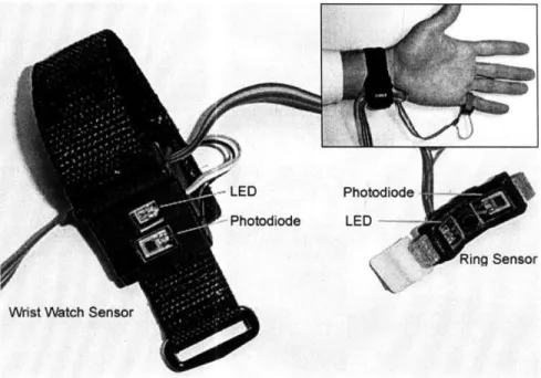
This thesis presents the design and development of a novel non-invasive BP monitor. The device provides beat-by-beat mean arterial blood pressure (MAP) estimates using adaptive calibration of the measured transit time of a propagating arterial pressure wave. The device employs unique wearable sensor architecture to estimate peripheral pulse transit time measurements. This architecture is comprised of two in-line photoplethysmograph sensors one in the form of a wristwatch measuring the volumetric pulsation in the ulnar artery and one in the form of a ring measuring the volumetric pulsation of the digital artery at the base of the little finger. Use of this architecture eliminates problems associated with the traditional method of estimating pulse transit time using the electrocardiogram (EKG). Additionally, by co-locating the two sensors on the same appendage not only are we able to account for the effect of hydrostatic pressure variation in our pulse transit time (PTT) measurements using an imbedded height sensor, but by actively altering the height of the two sensors relative to the heart we can achieve real-time identification of the calibration equation mapping PTT to MAP. Such real-time calibration of PTT measurements obviates the need for obtrusive cuff-based blood pressure monitors and offers the potential to recursively update the calibration equation as the patient's cardiovascular state evolves throughout the duration of the measurement period. Adaptive PTT calibration through natural patient motion has never previously been explored and offers the potential to achieve the longstanding goal of a truly imperceptible, wearable home BP monitor.

This thesis describes the design and development of the sensor hardware used in the wearable device. Based on both theoretical study and experimental observations a device model has been developed to allow estimation of mean arterial blood pressure using the pulse transit

times measured with our sensors. Additionally, this thesis presents the adaptive calibration methodology and the novel system identification algorithms that were used to parameterize our device model using natural human motion. Finally, this thesis demonstrates the potential of these innovative concepts through human subject testing and data analysis.

Thesis Committee: Chair

H. Harry Asada, Ph.D.

Ford Professor of Mechanical Engineering Roger G. Mark, M.D. Ph.D.

Distinguished Professor in Health Sciences and Technology, Professor of Electrical Engineering Andrew Reisner, M.D.

Visiting Scientist in Health Sciences and Technology and Attending Physician at Massachusetts General Hospital in the Department of Emergency Medicine

Warren Seering, Ph.D.

ACKNOWLEDGMENTS

I owe a great deal of thanks to a lot of people because without their support and friendship I could never have completed this thesis. In addition to furthering my professional development which culminated with the completion of my doctoral degree, my years at MIT have been a time of significant personal growth and I will always be thankful for all the opportunities that life as a graduate student here afforded me.

I would like to thank Professor H. Harry Asada my thesis advisor, whose guidance and financial support fostered my development as a researcher and engineer.

I would like to thank Dr. Andrew Reisner who initially championed the idea behind my thesis research and whose knowledge of medicine and cardiovascular monitoring provided me with numerous insights and inspiration.

I would like to thank Professor Roger Mark whose initial skepticism, tough questions, and medical insight proved an invaluable asset towards the development of my work.

I would like to thank Professor Warren Seering for his contributions to my thesis work as a member of my thesis committee.

I want to offer a big thank you to Dr. Timothy Davis for all of his advice and insight both of which served as priceless assets in the completion of this thesis.

Thanks to all the students of the d'Arbeloff Lab both past and present who became my good friends, opened my eyes to different perspectives, and made those long hours in the lab a little easier. Thanks to all of you for offering me a friendly ear when I needed it.

A special thanks to all my friends in the Cambridge Surf Crew, you all have become like family to me over the years and proven to me that a person can be both a successful student and still be a dedicated surfing, skiing, and snowboarding hellman. You all helped me to get through MIT "my way".

Also I would like to thank all the MIT sand volleyballers, I will truly miss summer time in graduate school.

Most importantly, I would like to thank my wife Lisa who has been my biggest supporter throughout the years. You have helped me get through both good times and bad, and never stopped believing in me. I am a very lucky man.

I would also like to thank my family for their support and encouragement throughout the years. And for helping me to believe that I could accomplish anything I set my mind to do.

I dedicate this thesis to the memory of my grandmother, Rowena McCombie who was a graduate of the University of California, Berkeley and who had a life long love of books and

TABLE OF CONTENTS

CHAPTER 1 INTRODUCTION 11

1.1 Wearable blood pressure monitoring 11

1.2 History & limitations of blood pressure estimation with pulse wave velocity 12 1.3 Adaptive calibration of peripheral pulse transit time 14

1.4 Thesis summary & organization 16

CHAPTER 2 DEVELOPMENT OF A PERIPHERAL PULSE TRANSIT TIME

17 DEVICE MODEL

2.1 Anatomy of the peripheral pulse transit path 17

2.2 Arterial pulse wave propagation 19

2.3 Arterial blood pressure & pulse wave velocity 21

2.4 A Lumped Parameter Model 32

CHAPTER 3 INSTRUMENTATION DESIGN & DEVELOPMENT 35

3.1 The photoplethysmograph signal 35

3.2 Sensor measurement site selection 38

3.3 Sensor housing design 44

3.4 Imbedded height measurement sensor 46

CHAPTER 4 PULSE TRANSIT TIME ESTIMATION 49

4.1 Pulse transit time estimation using blood pressure waveforms 49 4.2 Pulse transit time estimation using photoplethysmograph waveforms 50 4.3 Potential pulse transit time estimation techniques 56

CHAPTER 5 ADAPTIVE HEIGHT CALIBRATION (AHC) 61

5.1 Relative height variation & pulse transit time 61

5.2 Principal equations 63

5.3 Adaptive system identification 67

5.4 Adaptive height calibration implementation 69

CHAPTER 6 AHC HUMAN SUBJECT TESTING 73

6.1 Experimental protocol 73

6.3 Evaluating Correlation Between Model Parameters 79

6.4 Data screening 84

CHAPTER 7 MODELING THE EFFECTS OF SENSOR CONTACT PRESSURE ON

87

MEASURED PULSE TRANSIT TIME

7.1 Understanding the influence of sensor contact force 87 7.2 External pressure dependent phase delay in the PPG 94

7.3 External pressure dependent pulse wave velocity 98

CHAPTER 8 FULL PTT CALIBRATION USING EXTERNAL ARTERIAL

113

PRESSURE VARIATION

8.1 External arterial pressure as a calibration tool 113 8.2 Transmural pressure estimation using relative height variation 114

8.3 Full calibration of a lumped parameter model 116

8.4 Identification ofyo using a wristwatch PPG sensor and ring PPG sensor 124

8.5 Implementation of the full calibration method 126

8.6 Sensitivity and Error Analysis 128

CHAPTER 9 FULL CALIBRATION HUMAN SUBJECT TESTING 135

9.1 Wrist Posture external pressure change 135

9.2 Experimental protocol 136

9.3 Transmural pressure estimation 138

9.4 Experimental results 140

CHAPTER 10 DISCUSSION 145

10.1 Improving the calibration routine 145

10.2 External pressure dependent correlation between PTT & height 147

CHAPTER 11 CONCLUSION 153

11.1 Summary of accomplishments 153

11.2 Future work 155

LIST OF FIGURES

Figure 1-1. Height based calibration of a non-invasive blood pressure sensor

Figure 1-2. Novel peripheral pulse transit time measurement device with dual in-line PPG sensors

Figure 2-1. Common arterial anatomy of the left hand

Figure 2-2. A comparison of the vessel area and the pulse wave velocity predicted by the Langewouters model & Hughes model

Figure 2-3. Hysteresis observed between blood pressure and volume in one cardiac cycle of a PPG waveform

Figure 2-4. Evaluating hysteresis between BP & PTT: experimental observation of intra-vascular pressure loading and unloading on pulse transit time measurements Figure 3-1. Operating principle of the PPG sensor applied to the digital artery of the

finger

Figure 3-2. The measured PPG voltage signal is inversely proportional to the underlying arterial pressure waveform.

Figure 3-3. Potential PPG sensor site locations

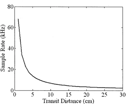
Figure 3-4. Required PPG sensor sample rate as a function of transit distance. Figure 3-5. Estimated pulse transit time error measured between the ulnar artery and

digital artery PPG sensors

Figure 3-6. Blood pressure estimation error as a function of the transit distance between the in-line PPG sensors

Figure 3-7. Key design elements used to develop a PPG sensor to measure arterial volume change

Figure 3-8. Timeline depicting milestones in prototype device design and testing Figure 3-9. Diagram and variables used in single accelerometer arm height estimation Figure 3-10. Comparison between height measurements made using a single 3-axis

accelerometer imbedded in the wrist sensor and a manometer

Figure 4-1. Estimated pulse transit time depends on the technique used to identify the arrival time of the PPG waveform

Figure 4-2. Model depicting the pressure dependent behavior of the compliance of the arterial wall

Figure 4-3. Variation in the arterial pressure volume relationship due to external loading Figure 4-4. Wrist PPG waveform data measured given an increase in sensor housing

pressure during each successive stage

15 16 18 25 27 28 36 37 38 40 42 43 44 43 47 48 51 53 54 55

Figure 4-5. Figure 4-6. Figure Figure Figure 4-7. 5-1. 5-2. Figure 5-3. Figure Figure Figure 5-4. 5-5. 5-6.

The effect of a multi-stage increase in external pressure on the shape of the wrist PPG waveform

Pulse arrival time estimation using the waveform threshold averaging technique

Pulse arrival time estimation using onset minimization

Observed alteration in pulse transit time caused by relative height variation Block diagram depicting the dynamic relationship between transmural arterial pressure and a measured non-invasive sensor signal

Transformation of a linear system with zero-mean output into an equivalent system with a zero-mean input using a linear filter

Block diagram depicting the adaptive height calibration algorithm

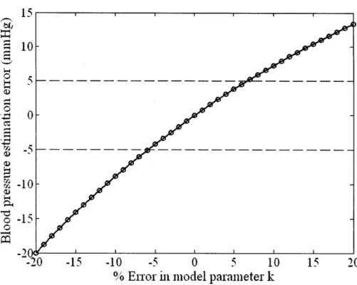
Blood pressure estimation error as a function of error in model parameter, k Relationship between model parameter error and calibration period length Figure 6-1. Sensor attachment configuration used in the adaptive height calibration tests Figure 6-2. Photo of a test subject during the initial phase of the AHC experimental

protocol

Figure 6-3. Experimental pressure variation measured at the wrist sensor during a human subject test

Figure 6-4. Histogram depicting the age distribution of the AHC test subject population Figure 6-5. Percent error between the model parameter k identified with AHC and k

identified with Finapres BP measurements

Figure 6-6. Sample human subject test result depicting the difference between PTT BP & Finapres BP

Figure 6-7. Sample of the actual and estimated contribution to the measured PTT caused by unknown blood pressure variation throughout the calibration period Figure 6-8. Variation in the identified model parameters, k and yO over a 9 hour period Figure 6-9. Model parameter variation observed in human subject data collected on two

consecutive days

Figure 6-10. Pulse transit time error may result from measurements made from PPG waveforms with a low signal to noise ratio

Figure 6-11. Pulse transit time error may result from signal abnormalities in the onset of the PPG waveform

Figure 7-1. Experimental variation in external wrist sensor pressure using a change in hand posture

Figure 7-2. Experimental variation in external wrist sensor pressure using direct pressure 91 on sensor housing

Figure 7-3. Measurement site anatomy subject to a sensor contact force, Fc 93 Figure 7-4. Block diagram displaying the dynamic relationship between arterial pressure, 94

external pressure, and the measured PPG signal

Figure 7-5. Voigt model used to describe the dynamic behavior of the arterial pressure- 96 volume relationship

Figure 7-6. Sketch of the pressure dependent arterial stiffness 97 Figure 7-7. Sketch of the distributed external pressure along the arterial transit path 99

observed by our in-line PPG sensors

Figure 7-8. Experimental configuration used during stage 1 of the Finger Band Test 100 along with the distributed external pressure along the arterial transit path

Figure 7-9. Example finger PPG data set measured before and after band removal during 102 the Finger Band Test

Figure 7-10. Pulse transit time estimates for a male subject derived form the EKG and 104 finger PPG before and after direct wrist sensor pressurization

Figure 7-11. The measured finger PPG signal before and after direct wrist sensor 105 pressurization

Figure 7-12. The measured wrist PPG signal before and after direct wrist sensor 105 pressurization

Figure 7-13. Multi-stage variation in external wrist sensor pressure using direct pressure 107 applied to the wrist sensor housing

Figure 7-14. Pulse transit time and PPG magnitudes fro a healthy male subject in response 108 to a multi-stage increase in external wrist sensor pressure

Figure 7-15. Distributed pulse wave velocity along the arterial transit path observed by 109 our in-line PPG sensors

Figure 7-16. Block diagram of the lumped parameter device model that includes the 111 effects of sensor contact pressure

Figure 8-1. External arterial pressure variation as a means to calibrate pulse transit time 113 Figure 8-2. Typical intra-arterial and extra-arterial pressure values fro a patient wearing 116

our PPG sensors

Figure 8-3. Pulse wave propagation through an artery under a uniform external pressure 117 Figure 8-4. Pulse wave propagation through an artery under two external pressures 119 Figure 8-5. Pulse wave propagation through an artery under three external pressures 122 Figure 8-6. Bi-stable sensor strap used to alter the pressure exerted on the ulnar artery by 127

Figure 8-7. Figure 8-8. Figure 8-9. Figure 9-1. Figure 9-2. Figure 9-3. Figure 9-4. Figure 9-5. Figure 9-6. Figure 10-1. Figure 10-2.

Full calibration routine combines relative height variation and external pressure variation

Calibration curves for diastolic pressure and mean arterial pressure Mean arterial pressure error due to variance in the identified model

parameters as a function of the calibration period

A change in external wrist pressure can be implemented using an alteration in hand posture

Hydrostatic pressure variation and the two external pressures implemented during the three-stage human subject tests

PPG magnitude estimated as the difference between the maximum and the minimum values of the PPG waveform during each cardiac cycle

Transmural pressure estimation using the maximum PPG magnitude and the measured height

Bland-Altman plot comparing the mean arterial blood pressure estimated by the adaptively calibrated PTT algorithm and the Omron cuff.

A comparison of beat-to-beat mean arterial blood pressure estimated using adaptively calibrated PTT and mean Finapres BP

Future calibration routines should separate height variation and estimation of the effects of external pressure change

The effect of external sensor pressure on the magnitude and estimated arrival time of various blood pressure waveform features in the wrist PPG

waveform

Figure 10-3. Picture of wrist sensor housing with a thin contact width Figure 10-4.

Figure 10-5.

Pulse transit time estimated from the wrist PPG waveform and EKG during multi-stage progressive increases in external wrist sensor pressure

The variation in PPG magnitude and pulse transit time are dependent on arterial compliance

Figure 11-1. Cyclic design and development process for a wearable BP monitor

128 130 134 135 137 138 139 142 143 146 148 149 150 151 155

CHAPTER

1

INTRODUCTION

1.1

WEARABLE BLOOD PRESSURE MONITORING

Hypertension or chronic high blood pressure is a major health issue in the United States. It is estimated that between 25%-50% of all adult Americans suffer from this condition [1,2].

Just as feedback from a scale helps people attempting weight loss to adhere to their diet and exercise regimen, patients suffering from hypertension are more likely to adhere to their doctor prescribed treatment when they regularly monitor their blood pressure.

Leading home blood pressure monitors work based on the principle of oscillometry and require an inflatable cuff to measure arterial blood pressure (BP). These cuff based devices permit episodic "snap-shot" measurements of arterial blood pressure while the patient is suspended in a stationary position. Although useful, a single snap-shot measurement of the time varying blood pressure, which fluctuates minute-by-minute, and from night-to-day is incapable of encapsulating the dynamic state of the cardiovascular system. Moreover, the existing BP devices are a chore: they are cumbersome, finicky [3,4], and uncomfortable [5].

Wearable blood pressure monitoring technologies may be able to overcome the drawbacks of existing home BP monitors, (burdensome stationary measurement periods and monitors providing limited snap-shot measurements). There are three levels of potential benefits to wearable blood pressure monitoring. First, extend the proven benefits of today's standard BP cuffs by making home BP monitoring less of a burden. Regular monitoring as a source of feedback has been shown to improve patient compliance with prescribed treatments [6,7]. Second, extend the benefits of intensive 24-hour ambulatory BP monitoring protocols to more patients, and more days per year, allowing better stratification of a patient's risk and tailoring of their prescribed treatment [8,9]. Third, exceed the benefits of intensive 24-hour ambulatory BP monitoring by measuring BP more frequently than every 15 minutes.

In order for a wearable BP device to realize these potential benefits it must meet a number of requirements. The monitoring device must operate unobtrusively and it must be compact, lightweight, and low power. Additionally, it must be capable of providing accurate measurements throughout its use and across changing cardiovascular states, thus the device must

have a means of self calibration. Finally, the wearable device must be able to provide continuous measurements while being worn by the patient.

A number of non-invasive blood pressure (NIBP) measurement methods exist, however none of the existing methods meet all the requirements listed above. A major short-coming of many of these non-invasive BP devices is their use of an obtrusive actuated cuff during device calibration and BP measurement. These actuated devices whether pneumatic or mechanical are not only obtrusive, requiring uncomfortable arterial compression for every measurement, but the actuators also significantly increase the power consumption of the devices. Leading NIBP methods in this category include sphygmomanometry, oscillometry, tonometry, and the volume clamp method of Penaz [10].

An alternative NIBP measurement method exists that is capable of estimating blood pressure without any actuators. This method estimates BP using calibrated pulse wave velocity measurements [10]. This passive method not only eliminates the need for an actuated cuff during measurement but also has the capability of providing continuous beat-to-beat BP estimates. As such, calibrated pulse wave velocity has the potential to satisfy the requirements of wearable monitoring and allow doctors and patients to finally realize the potential benefits of a wearable device. However, pulse wave velocity is not without its shortcomings and several key limitations must be addressed in order to utilize it in a wearable monitor.

1.2

HISTORY

&

LIMITATIONS OF BLOOD PRESSURE ESTIMATION

USING PULSE WAVE VELOCITY

The study of pulse wave velocity (PWV), the speed at which a pressure pulse is transmitted from the heart through the arterial tree has a long history. The relationship describing the propagation of pressure waves in an elastic tube e.g. a blood vessel, was first described separately by Moens and Korteweg in 1871 [11]. Their seminal work was later confirmed and extended by Bramwell and Hill in 1923 [11]. The utility of pulse wave velocity as a surrogate measure to estimate arterial blood pressure has been the subject of research since the 1960's. Since then there has been extensive academic and commercial effort to use this as a monitoring modality. Yet the accuracy of PWV based BP monitors has been suboptimal e.g. [12]. Per

Chen, "No one has succeeded in realizing a reliable blood pressure monitor when only the pulse wave velocity or pulse arrival time is used [13]."

The difficulties associated with using pulse wave velocity to estimate BP can be divided into two general categories, (1) inaccurate measurement of PWV using non-invasive sensors and (2) employing static calibration equations to map the PWV measurements to BP.

Existing blood pressure estimation methods based on pulse wave velocity rely on measurement of pulse transit time (PTT), the time required for the pressure pulse to travel between two different locations along the arterial tree, and either implicit or explicit measurement of pulse transit distance (Ax). Their relationship is given in (1.1).

Ax

pwv - _(1.1)

ptt

The vast majority of existing PWV devices define and measure the pulse transit time, as the time elapsed between the apex of the R wave of the electrocardiogram (ECG) and the arrival of the photoplethysmograph (PPG) waveform signal in the finger tip. However, the ECG has been shown to be a problematic marker when used to indicate the onset of the pressure pulse as it emanates from the left ventricle because of variations in the electromechanical delay in the heart

[37]. These undetectable variations in the delay will cause variations in the measured PTT that

are unrelated to arterial blood pressure and thus act as sources of BP estimation error.

Other alternative PTT estimation methods have also proved problematic. The difference in pulse arrival times measured between two PPG waveforms placed at distinct locations on the body, e.g. the finger and the toe, or the finger and the ear have been investigated as a potential proxy metric for BP estimation. Although the difference in pulse transit time measured from these two sensor architectures demonstrated some correlation with changes in systolic (peak) BP the difference did not exhibit a correlation with changes in diastolic (minimum) BP [12,14,15] and limit this measure's utility.

Hydrostatic pressure variations caused by postural changes or elevation change in the extremity where PPG measurements are derived have been shown to influence the measured PTT [15]. If not accounted for, the influence of hydrostatic pressure on measured PTT can serve as a source of error in estimating central BP and may make BP estimates using ECG and PPG unreliable in any position except supine [16].

Pulse wave velocity devices also suffer from a difficulty to accurately measure the pulse transit distance between the two sensor locations. Although the transit distance can be lumped into model parameters identified during initial device calibration it is difficult to keep this distance constant [18] and this imprecision creates another source of error in BP estimation using PTT alone.

Although the use of the ECG and the effects of postural variation may serve as sources of BP estimation error, perhaps the most significant limitation to current PWV technologies is caused by the use of a static calibration equation to map PTT measurements to BP given the dynamic properties of the arterial walls.

Leading pulse wave velocity blood pressure monitors require a calibration equation relating PTT to BP to be identified and parameterized for an individual prior to using the device to estimate BP. This calibration equation is generally identified using a set of training data in which blood pressure measurements from an actuated device (e.g. a cuff-based sphygmomanometer or oscillometer) are collected simultaneously with pulse transit time measurements [17]. Once the parameters of this calibration equation have been determined they are assumed to remain constant throughout the estimation period. However, the relationship between PWV and BP is a function of the patient's vascular physiology (e.g. arterial stiffness) which can be altered by changes in vascular smooth muscle tone [18]. Therefore, the equation relating PTT to BP for any individual is dynamic and changes in conjunction with changes to the patient's cardiovascular state. Thus, accurate estimation of BP using PTT requires that a device update parameters in a dynamic calibration equation across changing physiologic states. Currently, there are no PWV devices that allow adaptive, on-line calibration of PTT to BP.

1.3

ADAPTIVE CALIBRATION OF PERIPHERAL PULSE TRANSIT TIME

Intravascular blood pressure is not only a function of the volume of fluid passing within the vessel lumen due to the contracting heart but it is also a function of gravity. The earth's

gravitational field creates a pressure difference (AP) along the arterial tree by acting on the columns of blood in the vessels [18], thus the arterial pressure in the foot is much higher than the pressure in the aorta when a person is standing upright. The magnitude of this effect is described by equation (1.2) where p is the blood density, g is the gravitational acceleration constant, and Ah the relative height of the fluid column formed between the heart and measurement site.

AP(t) = pgAh(t) (1.2)

Gravity's effect on arterial blood pressure can be exploited in order to calibrate a wearable sensor. Placement of a wearable blood pressure sensor at a peripheral location such as on the wrist or finger allows adjustment of the intravascular pressure at the sensor's measurement point by moving the sensor to different heights relative to the height of the heart. The change in intravascular pressure at the measurement site is equal to the pressure change predicted by (1.2) and can be directly estimated using measurements of the sensor's height relative to the heart as depicted in Figure 1-1. A comparison of changes in intravascular hydrostatic pressure to the observed changes in the sensor's output permits calibration of the non-invasive measured parameter, or height based calibration.

Height based calibration was originally utilized by Shaltis and Asada [19] in a modified form of oscillometry. In their method they proved that the external sensor contact pressure acting on the artery at the measurement site could be reduced and maintained below mean arterial pressure and the maximum PPG pulsation amplitude could still be identified using height variation. However, their method still required a cumbersome, lengthy calibration procedure, an actuated pressure sensor stage, and did not allow continuous BP estimation.

The full potential of this novel height based calibration tool can only be realized when this technique is combined with an innovative device based on a passive NIBP principle and with sophisticated signal processing algorithms that provide a means to adaptively calibrate the device using a patient's natural motion. A combination of this set of enabling technologies could truly deliver an unobtrusive, self-calibrating BP monitor [20].

1.4

In this thesis I will describe the development of this set of enabling technologies. I will describe a novel method for estimating arterial blood pressure based on pulse wave velocity. This new method will employ a unique sensor architecture that is comprised of two in-line PPG sensors to estimate pulse transit time, one located above the ulnar artery at the wrist and one located along the base of the little finger above the digital artery (Figure 1-2). Use of this architecture will eliminate problems associated with estimating PTT from the ECG and because of their close proximity will simplify measuring the pulse transit distance. Additionally, by co-locating the two sensors along the same appendage not only will we be able to account for the effect of hydrostatic pressure variation on our measurements, but by actively altering the height of the two sensors relative to the heart, height based calibration can be used along with novel signal processing techniques to adaptively identify the calibration equation mapping PTT to BP. This thesis details the development of an in-line PPG based device model relating PTT to BP, the design of the novel PTT device, potential methods for estimating PTT with the PPG waveforms are evaluated, it presents the system identification algorithms used to identify device model parameters using natural motion, and presents initial human subject test results obtained using the novel device and identification algorithms.

-LED

r- Photodiode

Photodio~e

LED n

Wrist Watch Sensor

Figure 1-2. Novel peripheral pulse transit time measurement device with dual in-line PPG sensors

Soli

CHAPTER

2

DEVELOPMENT OF A PERIPHERAL PULSE

TRANSIT TIME DEVICE MODEL

The goal of this chapter of the thesis is to describe the development of a lumped parameter model governing pulse wave velocity in the peripheral arteries monitored by our in-line PPG sensors. The model must characterize the relationship between the measured pulse transit time, the arterial blood pressure, and the pressure change produced by relative height variation.

The development of this model begins by understanding the anatomy of the arteries that form the transit path between the two sensors. Based on a number of assumptions a one-dimensional wave model will be developed to describe the velocity of a pressure pulse in an elastic vessel. The validity of the assumptions used to develop this one-dimensional model will be explored in the context of the peripheral arterial anatomy and the pulse wave velocity model will be augmented to characterize the important features of the arteries that form the transit path. Finally, a lumped parameter model that will be utilized by our device to estimate arterial blood pressure from measured pulse transit time will be presented.

2.1

ANATOMY OF THE PERIPHERAL PULSE TRANSIT PATH

Operation of our novel BP monitor utilizes PTT derived from PPG waveforms recorded from the ulnar artery (PPG 1) at the wrist and from the common palmar digital artery on the outside of the little finger (PPG 2) as shown in Figure 2-1.

As the left ventricle ejects blood from the heart a pressure pulse wave is transmitted along the arterial tree propagating towards our two PPG measurement sites in the left hand. The path of the pulse wave begins in the ascending aorta, propagating next along the aortic arch, continuing into the left subclavian artery, then along the axillary artery, and into the brachial artery of the upper arm. The brachial artery splits just below the elbow joint into two branches, the ulnar and radial arteries. The pressure pulse wave propagates through both of these arteries into the arteries of the hand.

I

I !

ARER PP

Figure 2-1. Common arterial anatomy of the left hand

The arteries in the hand form a complex network of inter-connected vessels that provide redundant paths along which the pulse wave can propagate and blood can flow. The most common configuration of the arterial network of the hand found in nearly 80% of the population

[21] is shown in Figure 2-1.

The primary paths of blood flow and wave propagation for the various arteries in the hand are displayed in Figure 2-1 using color coding. Arteries displayed in red are primarily supplied by the ulnar artery. The ulnar artery primarily supplies blood to the little finger. In this path blood flows from the ulnar artery into both the common palmar digital artery on the outside of the little finger and into the superficial palmar arch, after passing into the superficial palmar arch blood flows into the common palmar arteries and then into the proper palmar digital arteries in the fingers. Arteries displayed in purple are primarily supplied by the radial artery. The radial artery is the primary blood supply for the thumb, index, middle, and ring fingers. After passing through the radial artery blood flows both into the deep palmar arch and into the princeps pollicis artery supplying the thumb and also into the radial indicis artery supplying the index finger.

Blood supplied to the deep palmar arch flows into the common palmar arteries and then into the proper palmar digital arteries in the fingers.

The primary wave propagation path observed by our device measures the transit time as a pulse wave propagates along the ulnar artery into the common palmar artery on the outside of the little finger. This path consists of one major arterial bifurcation as the ulnar artery branches into the palmar digital artery and also continues into the superficial palmar arch.

Although other anatomical configurations of the arterial network in the hand do exist [21], none of the most common configurations alter the propagation path of our device. However, we should be aware that in a very small minority of the population this propagation path may exhibit some variation.

2.2

ARTERIAL PULSE WAVE PROPAGATION

The framework for understanding the relationship between arterial pulse wave velocity and blood pressure begins with an analysis of wave propagation in a circular, cylindrical, fluid-filled

tube given a number of simplifying assumptions [11,22], these assumptions are listed below.

Tube Assumptions: Fluid Assumptions:

* Infinitely long * Homogeneous

* Straight * Incompressible

* Isolated * Nonviscous

* Elastic

* Negligible mass

The continuity equation for the fluid in an elastic tube with cross-sectional area A(z, t) having an average flow velocity in the axial direction U(z, t) is given in (2.1).

aA a

-+ -(UA)= O (2.1)

at az

The definition of cross-sectional area in a circular tube can be used to transform (2.1) into an expression involving tube diameter, D(z, t) as given in (2.2).

D2 a UD)= 0 _(2.2)

at az

Using the product rule the partial derivatives in the expression in (2.2) can be expanded into the expression given by (2.3).

D

O D 2 U

2D + U2D -+D 2 =0 (2.3)

at

az

az

Assuming the wave amplitude is small and the wavelength is long compared to the diameter of

aD

the tube the slope of the tube, <<1 and this term in (2.3) can be neglected resulting in the

az

expression given by (2.4).

+ =0 (2.4)

D at 6z

The equation of motion for the fluid in the tube with density p and internal tube pressure

Pi is given in (2.5).

aU

au 1 P~

+- + - = 0 (2.5)

at

az

p az

Under the assumption that the fluid velocity U is small the second term in (2.5) can be neglected and the expression reduced to the equation given by (2.6).

a U 1 BP

+

=0

(2.6)

at p

az

Equations (2.4) and (2.6) along with a constitutive equation for the tube wall, describing the relationship between transmural pressure, Ptm and tube diameter D, form the basic set of equations used to model wave propagation in an elastic tube.

Continuation of the analysis requires an assumption regarding the tube wall's constitutive model. Based on the theory of thin shells [22] the dynamics of the model can be eliminated by neglecting the mass of the tube and ignoring any partial derivatives leaving a simplified algebraic relationship as given by (2.7).

D = fcn (P, (z,t)) (2.7)

Given this algebraic model the chain rule can be used to expand the partial time derivative of diameter in terms of the transmural pressure as given by (2.8).

aD dD dPt

aD

dD-

The expression in (2.8) can be substituted into (2.4) leaving a simplified continuity equation as

tm+

at

2

dD

.z

The transmural pressure acting across the tube wall is defined as the difference between the internal pressure Pi, and external pressure Pex as given in (2.10).

P,, = P, - P. (2.10)

Substituting the definition of transmural pressure into the partial time derivative term in (2.9) and under the assumption that the external pressure is constant simplifies the continuity equation further as given by (2.11).

8

+

_{D dm}

_PU

_U

₌

at 2 dD 8z

Although alternative models describing the relationship presented in equation (2.7) will be considered in Section 2.3 the remainder of this analysis assumes that the elastic tube is thin walled and the wall material is a linear elastic solid that obeys Hooke's law. The circumferential strain e, in a tube wall experiencing small changes in the inner tube diameter D is given by (2.12).

dD

(2.12) D

The wall strain induces a change in incremental tension dT, across the wall as given by (2.13) where E is the Young's modulus of the wall and h is the wall thickness.

dD

dT = hEe = hE dD _(2.13)

D

An equilibrium condition requires the tension in the wall be balanced by a change in the transmural pressure acting across the wall this balance is given by (2.14).

dD

2hE = DdPt (2.14)

D

This balance leads to the useful expression given by (2.15).

dPt dtm 2hE2hE

(2.15)

dD D'

The expression in (2.15) can be substituted into the continuity equation given in (2.11) deriving a new expression which is given in (2.16).

8P1 ₊ hE 8U_{hE =0 (2.16)}

at

D

The final wave equation describing pressure propagation in the tube can be developed by taking the partial derivative of equation (2.6) with respect to the axial coordinate z, and by taking the partial derivative of equation (2.16) with respect to time and then equating the mixed partial

derivatives to combine these equations as given by (2.17).

z

0

(2.17)

az

_hE

_at

The expression in (2.17) is an example of the well known wave equation (2.18).

,z

-(

-

=

0

_(2.18)

az

at

The definition of wave speed c, in the elastic tube is given in (2.19). This expression is the famous Moens-Korteweg equation.

c = (2.19)

pD

An alternative expression for the velocity of wave propagation (c) in an elastic tube can be developed from the Moen-Korteweg equation [11] or based on the analysis of sound wave propagation in air which was first studied by Isaac Newton. Newton's equation is given in (2.20) where B is the bulk modulus and p the density of the fluid.

c =C (2.20)

Substituting the definition of the bulk modulus into (2.20) for a tube with cross-sectional area A, and unit length provides an alternative equation for wave propagation in an elastic tube as given

in (2.21).

C Ad Pm (2.21)

2.3

BLOOD PRESSURE

&

ARTERIAL PULSE WAVE VELOCITY

Although the derivation presented in section 2.2 provides a framework for studying arterial pulse wave propagation it relies on a number of assumptions that are clearly violated by the vessels of the arterial system. In fact, these vessels are finite in length which results in wave

reflection; they demonstrate viscoelastic behavior including hysteresis, stress relaxation, and creep that suggests the need for a dynamic model, and exhibit pressure dependent non-linear elasticity, a characteristic exploited for non-invasive pressure estimation using pulse wave velocity. Additionally, blood is a viscous, non-Newtonian fluid, these fluid properties along with the damping characteristics of the viscoelastic vessel wall may cause attenuation of the pressure pulse as it propagates along the arterial path.

In this section the effects that these non-ideal behaviors have on wave propagation in the ulnar and common digital arteries will be considered and operating conditions given for when these behaviors can be neglected.

Perhaps the most important behavior of the arteries that must be reflected in our model is the non-linear relationship that exists between arterial blood pressure and the elasticity of the arterial wall. The stress-strain relationship of the arterial wall is a complex three-dimensional function. However, this function can be simplified and reduced down to two dimensions by considering only mean stresses in the vessel wall and by neglecting any transverse shear stresses [39]. The following discussion is based on the use of a two dimensional model given these assumptions.

The static elastic modulus (E), of the arterial wall in both human and canine arterial segments has been experimentally studied both in vivo and in vitro [23,26,27,28]. Based on these studies two leading empirical relationships have been presented to described the pressure dependence of the static elastic modulus.

Langewouters [28] developed a three parameter arctangent model to describe the relationship between arterial cross-sectional area (A) and transmural pressure (Ptm) in the abdominal and thoracic aorta of humans as given in (2.22) where Am is the maximal vessel area,

Po is the pressure at maximum compliance, and P1 is the pressure when the compliance is equal to half its maximum value.

A(Ptm) = + arctan (2.22)

This equation is based on the observation that the incremental Young's modulus increases with pressure according to a second order polynomial function as given in (2.23).

1 dP +C

E = -

dP

cP

Experimental results presented by Gizdulich [27] characterizing the pressure-volume relationship in the arteries of the forearm show that the model described by (2.22) can be used to represent the relationship between pressure and cross sectional area in these arteries. Experimental results by Langewouters [26] characterizing the pressure-diameter relationship in the arteries of the finger, also qualitatively demonstrated the behavior predicted by these equations.

The relationship in (2.22) can be combined with the definition of pulse wave velocity given by equation (2.21) to provide an expression for arterial pulse wave velocity as given by

(2.24).

1 1 1 P-Po dP

c

- - + - arctan

m

(2.24)

p 2 1 P dA(Ptm)

Although, none of the aforementioned authors provided a comparison between actual pulse wave velocity measurements in these arteries and pulse wave velocity values predicted using the model described in (2.24), they do provide empirical observations about the static elastic modulus of the arteries monitored by our device and they provide insight regarding the behavior of pulse wave velocity at zero transmural pressure in these arteries.

A popular and more tractable alternative expression for the static elastic modulus (E) of the arterial wall was developed by Hughes et al [23] based on experimental observations of the canine thoracic and abdominal aorta both in vivo and in vitro. In their experimental procedure the arterial diameter and wall thickness were measured using intravascular ultrasound and pulse wave velocity was measured using two catheter tip pressure sensors spaced a known distance apart. Their observations suggested an empirical relationship for the elastic modulus of the form given by (2.25).

E = E0 exp(aPm) (2.25)

Hughes showed that the elastic modulus values derived from the canine aorta demonstrated a correlation coefficient in excess of 0.95 with values predicted using the model in (2.25) when estimated with mean distending pressure measurements.

Hughes derived the expression for elastic modulus of the in vivo aorta based on the Moens-Korteweg equation given by (2.19). The two equations can be combined to describe a relationship between pulse wave velocity and arterial blood pressure [11 ] as given by (2.26).

c = hE° _exp(aP,,)

(2.26)

This equation suggests that arterial pulse wave velocity increases exponentially with an increase in transmural pressure. However, this exponential relationship is only valid for transmural pressure values equal to or greater than zero and may not provide physiologically meaningful pulse wave velocity predictions for transmural pressures below zero.

Although the Hughes model was not derived from peripheral arteries as was the Langewouters model, the two models predict very similar behavior in regards to the pressure cross-sectional vessel area relationship of the artery and the pressure pulse wave velocity relationship of the arterial wall as shown in Figure 2-2. Since both models describe similar behavior, the Hughes model which provides a more tractable mathematical expression than the Langewouters model will be used to characterize the static elastic modulus of the peripheral arteries in our lumped parameter model. However, predictions made with the Hughes model may not be valid for extremely negative transmural pressure values.

Cross-sectional Area

Pulse wave velocity

Figure 2-2. A comparison of the vessel area and the pulse wave velocity predicted by the Langewouters Model & the Hughes Model

- Langewouters Model --- Hughes Model h1 "-4 ri2 wl dI) -100 -50 0 50 100 Pressure (nunHg) lU 9 8 - 7 C)45 4 3 -100 -50 0 50 100 Pressure (nuniHg) x 10.4

·-,,

In addition to the exponential pressure dependence of the elastic modulus, both the wall thickness h, and inner vessel diameter D, are pressure dependent terms. However, their ratio

(h/D) can be shown to be relatively constant across a wide physiologic range of transmural

pressures. The diameter, D in (2.26) refers to the inner diameter of the vessel, which we will now refer to as Di. The wall thickness can be defined in terms of the inner vessel diameter and the outer vessel diameter Do as given in (2.27).

h = DO - D, (2.27)

Substitution of this expression into the ratio (h/D) yields the equation given in (2.28).

h - -D =(D - 1 _(2.28)

D D,

D,

The effect that transmural pressure has on the ratio of outer vessel diameter to inner vessel diameter may be examined given the assumption that the vessel wall volume remains constant as the vessel diameters change throughout the physiologic blood pressure range [39]. The definition of vessel wall volume (V,) for a unit length of vessel is given in (2.29).

Vw = 4(D2 - D2 ) (2.29)

Using equation (2.29) a comparison can be made between vessel diameters at time t1 and vessel diameters at a different time t2 as given in (2.30).

S(t) D(t))= (t) - D(t 2)) (2.30)

4

4

According to published data [11] the internal radial pulsation of the aorta during its transition between diastolic pressure and systolic pressure (-50 mmHg) is between 3-4%. The arterial walls of peripheral arteries such as the ulnar artery and common digital artery are less compliant than the aortic wall [22] therefore we would expect the internal radial pulsation in these arteries to be even smaller. Given the non-linear behavior of the arterial wall a liberal estimate of the total radial pulsation in these arteries as transmural pressure varies across the operating range of our device is approximately 10%. Under this assumption a relationship can be defined between the minimum inner vessel diameter (Di,mi,) and maximum inner vessel diameter

(Di,max) as given in (2.31).

Substituting this expression into equation (2.30) and equating the vessel wall volume at the maximum and minimum diameters allows derivation of an expression for the maximum outer vessel diameter as given in (2.32).

D

Using a mean value for ulnar artery diameter (Dmi = 2.5mm) [21] and assuming an ulnar artery wall diameter-thickness ratio of 12 (D/h = 12) for the minimum diameter similar to the radial

artery [29] using (2.31) and (2.32) we can calculate the outer to inner diameter ratios as given in (2.33). The percent change between the two ratios is less than one percent.

Dp D

D'ma = 1.07 o,mif

=

Therefore this ratio may be assumed constant with respect to transmural pressure with very little loss in accuracy using the model described in (2.26).

Along with nonlinear elasticity, the arterial wall demonstrates viscoelastic behaviors including hysteresis, and stress relaxation. This suggests that a dynamic equation is required to characterize the behavior of the arterial wall. Hysteresis is observed in the pressure-volume relationship in the artery. Therefore the arterial pressure and its corresponding arterial volume depend on whether the arterial pressure is increasing or whether it is decreasing. The plot in Figure 2-3 depicts the hysteresis that is observed between the arterial blood pressure, measured with a Finapres BP monitor, and the measured volumetric PPG signal during one cardiac cycle. The sample frequency was 1 kHz.

-V.YO -0y98 1.02 a -1.04 -1 A0 S 10 2 14 --80 100 120 140 160 Blood Pressurse (mnHg)

Figure 2-3. Hysteresis observed between blood pressure and volume in one cardiac cycle of a PPG waveform

ading doading --Jl_ .Vv, J .u

The pulse wave speed equation given in (2.21) shows that PWV is dependent on arterial volume, therefore this equation suggests that the relationship between pulse wave velocity and pressure may exhibit hysteresis and a dynamic equation may be necessary to characterize the magnitude of its effects on our pressure dependent pulse wave velocity as we load and unload the artery using height variation. The effect of this loading and unloading in the pressure-pulse wave velocity relationship was determined experimentally. Pulse wave velocity measurements were taken using our in-line PPG device while diastolic blood pressure was measured simultaneously using the Finapres blood pressure monitor attached to the index finger. During the experiment the height of the sensor measurement points were adjusted by raising and lowering the arm to

alter intravascular hydrostatic pressure. A typical result of these experiments is given in Figure

2-4. Although the figure depicts some variation in PTT due to the inherent transit time

measurement error using our in-line PPG sensors, hysteresis was not observed between the measured pulse transit time and diastolic blood pressure as the artery was loaded and unloaded. These experimental results suggests that the dynamic behavior of the arterial wall may be neglected when characterizing the behavior of pulse transit time induced by the loading and unloading of the wall as intravascular arterial pressure is altered by height variation during device calibration.

4

3.5

2t0

80

100

120

Diastolic Pressure (mmHg)

Figure 2-4. Evaluating hysteresis between BP & PTT: experimental observation of intra-vascular pressure loading and unloading on pulse transit time measurements.

·

loading

unloading

Sx

xo 20

In addition to hysteresis, the viscoelastic arterial wall also exhibits the phenomenon of stress relaxation. Therefore any stress imposed in the arterial wall under a constant strain will diminish over time. The result of this behavior is that changes in intravascular volume produced by altering the height of the sensor measurement point may remain constant but the instantaneous arterial pressure may diminish over time if the height is held constant. Since we have shown that the wall thickness - vessel diameter ratio in our model may be considered to be relatively constant over wide pressure ranges stress relaxation should not be a large issue. Despite the assumed insensitivity in our model, the effects of stress relaxation in the arteries underlying our sensors may be considered in the design of a height variation protocol used to identify the parameters of our device model.

To understand the impact of stress relaxation, a stress relaxation model describing the stress T, in the arterial wall in response to a step change in strain [39] is given in (2.34) where 7_{(e) is a function of strain or wall stretch ratio X.}

T(t, 2)= G(t)* T(e) (A) (2.34)

The normalized relaxation function G(t) in (2.34) is defined as given in (2.35). This function with constants 91 and d has been shown to be a useful approximation for times less than 100 seconds.

G(t)= 91 log(t)

+

d

(2.35)

Since the stress in the arterial wall is directly proportional to the transmural pressure acting across it the stress variables T and 7<e) can be replaced with corresponding transmural pressure terms Pt, and P.(e) as given in equation (2.36).

P,m (t, 2) = (w log(t)+ d)Ptm(e) (2) (2.36)

Based on experimental observation [39] the decay of the normalized relaxation function requires on the order of 100 seconds. Thus the effect of these slow dynamics may be neglected in our parameter identification by choosing a height variation frequency that is an order of magnitude faster than this time period (T-10-15 seconds).

Based on the previous analysis our device model will assume that the dynamics of the viscoelastic arterial wall are negligible.

In addition to neglecting the viscoelastic properties of the arterial wall, derivation of the Moens-Korteweg equation (2.19) assumes that the fluid in the tube is an inviscid liquid however

arterial wave propagation occurs in vessels filled with blood which is a non-Newtonian viscous fluid. The one dimensional wave model and the Moens-Korteweg equation remain valid representations of wave propagation in arteries where the Reynolds number and Womersley number are large. Under these assumptions boundary layer theory can be used to conform to the no-slip condition on the vessel wall imposed by a viscous liquid and still allow the ideal fluid assumption of our previous derivations. The definition of Reynolds number along with approximate values for the ulnar artery and common digital artery are given in (2.37a) and

(2.37b) respectively. Note that flow velocity U is assumed to be the mean velocity during the

cardiac cycle and that viscosity of blood is not fixed rather it is dependent on hematocrit (% of blood volume occupied by red blood cells) and shear rate.

Re _Re D

m

_ 1060 0.20 - - m

pUD

m

Re

-)14).950

dP 3.4 x 10-4Pa. s

The definition of Womersley number along with approximate values for the ulnar artery and common digital artery are given in (2.38a) and (2.38b) respectively.

. . 211'

a =D =

rad kg

a __ se )(06 m6.6 (2.38b)

Sa=1000

3.4

10

Pa.s

According to Fung [21] as the Reynolds number and/or Womersley number approach 1 or drop below 1 viscosity must be taken into account. Based on the values presented above for these dimensionless parameters it appears that the ideal fluid assumption is valid in these arteries. However, there is not a clear distinction or threshold between when the ideal fluid theory is valid and when viscous effects begin to play a role and some consideration should be

made to understand the potential errors that neglecting their effects could have on our pulse wave propagation model.

In addition to the viscous effects of the fluid, energy dissipation will also occur in the propagating wave due to the viscoelastic arterial wall [21]. The potential results of these two sources of energy dissipation are a reduction in pressure magnitude along the length of the vessel such that intravascular pressure along the length of the artery between the two sensors is not

BP.

constant a # 0 and/or a deceleration of the propagating pulse wave as it travels along the artery such that wave speed is not constant in the arterial segment between the two sensors. Because of the short transit distance between the two pulse waveform sensors in our device and the minimal dissipation predicted by the values in equations (2.37) and (2.38) these phenomenon will be neglected in our pulse wave speed model.

The final assumption that must be removed from equation (2.19) when considering arterial wave propagation is that the vessels are finite in length. This finite length results in pressure pulse wave reflection at locations having an impedance mismatch such as the arterioles. Therefore intravascular pressure at any point P is a result of the superposition of incident pressure waves PIN, and reflected pressure waves PRE as given in (2.39).

P = PI + PR (2.39)

A central problem associated with wave reflection is that the measured pulse waveform at any location along the artery is the result of an interference pattern created by the superposition of incident and reflected pressure waves as they propagate throughout the arterial tree. Therefore, a specific waveform feature e.g. maximum value, in the measured waveform is not representative of either the incident or reflected waveform alone. The two primary implications of this phenomenon are that the pulse transit time and pulse wave velocity estimated from two measured waveforms could represent an apparent pulse wave velocity (c') not the actual pulse wave velocity (c) described in (2.26) and this apparent pulse wave velocity would be frequency dependent.

A simple solution to this problem is to calculate pulse transit time measurements using only the wave front or leading edge of the waveform prior to the arrival of any reflected waves at the measurement site. The wave front velocity during this initial period is representative of the actual pulse wave velocity that is governed only by the properties of the arterial wall and has

pressure dependence described by the expression in (2.26). This solution assumes that the reflected and re-reflected waves have been attenuated to a negligible magnitude at the onset of the new pulse wave at our measurement site. Implementation of this method will be described further in chapter 4. An interesting aspect of our device is that due to the peripheral location of our sensor the time difference between incident waveform onset and arrival of the reflected pressure wave will be very brief. Assuming a reflection site in the finger tip (-5 cm) and a pulse wave velocity of 7 m/s, this time difference may be as brief as 7 milliseconds for the waveform measured by the ring PPG sensor.

2.4

A LUMPED PARAMETER MODEL

Based on the equations and analysis presented in the preceding sections a very simple pulse wave velocity model can be developed for our device. The pulse wave velocity through the arterial segment monitored by our device will be represented using the symbol 'pwv'. The expression in equation (2.26) can be simplified using the assumption that the pulse wave velocity at zero pressure (pwvo) is constant as given in equation (2.40).

pwv(Pm( = 0) = h = pwvo (2.40)

The expression in (2.26) can be further simplified by defining the constant parameter k as given in (2.41).

k = (2.41)

2

The expressions in equations (2.40) and (2.41) can be combined with (2.26) to form a lumped parameter model for pulse wave velocity in the peripheral arteries as given in (2.42).

pwv(t) = pwvo exp (k -Pm (t)) (2.42)

The relationship between pulse wave velocity and the pulse transit time (denoted using the symbol 'ptt') across an arterial segment of length Az is given in equation (2.43).

Az

ptt(t) = (2.43)

pwv(t)

The expression in (2.42) can be transformed into an expression using equation (2.43) to form a lumped parameter model between pulse transit time and transmural pressure as given in equation