Evaluation of the real contact area in three-body dry friction by micro-thermal analysis

HAL Id: insu-00447732

https://hal-insu.archives-ouvertes.fr/insu-00447732

HAL is a multi-disciplinary open access archive for the deposit and dissemination of sci-entific research documents, whether they are pub-lished or not. The documents may come from teaching and research institutions in France or abroad, or from public or private research centers.

L’archive ouverte pluridisciplinaire HAL, est destinée au dépôt et à la diffusion de documents scientifiques de niveau recherche, publiés ou non, émanant des établissements d’enseignement et de recherche français ou étrangers, des laboratoires publics ou privés.

Evaluation of the real contact area in three-body dry

friction by micro-thermal analysis

Philippe Stempflé, Olivier Pantalé, Toufik Djilali, Xavier Bourrat, Jamal

Takadoum

To cite this version:

Philippe Stempflé, Olivier Pantalé, Toufik Djilali, Xavier Bourrat, Jamal Takadoum. Evalua-tion of the real contact area in three-body dry fricEvalua-tion by micro-thermal analysis. 36th Leeds-Lyon Symposium Special Issue: Multi-facets of Tribology, Sep 2009, Leeds-Lyon, France. pp.1794-1805, �10.1016/j.triboint.2009.12.001�. �insu-00447732�

Evaluation of the real contact area in three-body dry friction by

micro-thermal analysis

Philippe Stempfléa, Olivier Pantaléb, Toufik Djilalib, Richard Kouitat Njiwac, Xavier Bourratd, Jamal Takadouma

aInstitut FEMTO-ST (UMR CNRS 6174 – Université de Franche Comté – CNRS – ENSMM

– UTBM), ENSMM, 26 chemin de l’Epitaphe, F-25030 Besançon Cedex, France

b Université de Toulouse, INP/ENIT, Laboratoire Génie de Production, 47 avenue d’Azereix,

F-65013 Tarbes, France

cInstitut Jean Lamour (MMNPS) – Dpt. SIMM – CNRS (UMR 7198) – INPL – Nancy

Université, Ecole des Mines, Parc de Saurupt, F-54042 Nancy Cedex, France

d Université d’Orléans, CNRS/INSU, Francois Rabelais Université de Tours ISTO, 1A Rue

de la Férollerie, F-54071 Orléans cedex 2, France

Abstract

Many tribological properties and wear mechanisms occurring on the micro-and nanoscale are strongly controlled by the so-called real contact area (Ar) which is a small fraction of the

nominal or apparent contact area (Aa). The determination of Ar is often based on either (i) a

geometrical approach describing the real geometry of contacting surfaces or (ii) a mechanical approach involving contact mechanics and physical-mechanical properties. In addition some experimental methods have also been attempted but they generally do not take into account the presence of third body at the interface—i.e. the wear debris trapped within the contact. In this paper we propose an experimental approach to estimate the dynamic real contact area from the operating parameters (Fn, v, T) and the tribological responses (μ, Ft) in presence of

third body. A scanning thermal microscope (SThM) is used for determining both the thermal conductivity of the third body and the relationship between the contact temperature and the thermal power really dissipated at the micro-asperity level. These results are combined with a thermal model of the macro-tribocontact for computing the real contact area and the real contact pressure. Validation of these results is carried out using a classical Greenwood Williamson model and finite element models built from the real AFM maps.

Keywords: Scanning thermal microscopy; Friction; Third body; Greenwood–Williamson approach

1. Introduction

Many tribological properties—such as friction and wear—greatly depend on the so-called real area of contact which is known to be only a small fraction of the apparent area of contact[1], [2], [3], [4] and [5]. In the absence of good measurement methods of the real contact area, the contact area is generally calculated using various models, built from different basic contact geometries, according to suitable hypotheses about the contact [6], [7], [8] and [9]. Thus, when the surfaces are assumed smooth—i.e. when the real contact area is the same as the apparent contact area—the hertzian's model[10] and the Mindlin's model[11] are respectively used in the case of the elastic contact when the shearing force within the contact is or is not negligible [12] and [13]. The JKR[14] and DMT[15] approaches are more suitable when the

adhesive forces are no longer negligible. However, practical surfaces are generally non-smooth because they always possess some degree of roughness [16] and [17]. Hence a real area of contact occurs between the asperities of surfaces in contact [3], [4], [5], [8] and [18] which is responsible of some tribological phenomena like elemental wear processes [19], [20], [21] and [22] or thermal-induced effects [23], [24], [25], [26] and [27]. From these observations, theories [3], [4], [5], [28], [29], [30], [31] and [32] have been developed considering in the same time the topography (mean radius curvature of the asperity summits and standard deviation of the summit heights [3] and [28], surface roughness power spectra [9], [16] and [31], fractal model [30] and [33]), the deformation constants (Young's modulus, hardness, yield stress…), the contact forces (load, friction and internal adhesive force), and the deformation regime of the asperities (i.e. elastic [3], [5] and [34], elasto-plastic [35], [36], [37] and [38], or fully plastic [39] and [40]). However, these theories are often difficult to apply in practice. First, they clearly depend on the deformation regime usually unknown at the scale of the real contact area. Second, some of the topographical parameters are rather

subjective and difficult to extract from the surface roughness (e.g. mean radius curvature of the asperity summits). Besides, in practice, a third body—i.e. the wear debris trapped within the contact—modifies continuously the power dissipated by friction through a dynamic real contact area [41] , [42] and [43]. Thus, in addition to the above theories, experimental methods have also been attempted using electrical resistance [44] and [45], optical methods and interferometry [46], adhesion and separation of sticky surfaces, phase contrast, total reflectance [47], or acoustic transmission [8].

The aim of this paper is to propose an experimental procedure to estimate the real contact area from the operating parameters (Fn, v, T) and the tribological responses—i.e. the power

dissipated by friction—in presence of third body. A scanning thermal microscope (SThM) [48], [49], [50], [51], [52] and [53] is used for determining both the thermal conductivity of the third body [54], [55], [56], [57], [58], [59] and [60] and the relationship between the contact temperature and the thermal power dissipated at the micro-asperity level within the interface [53], [61], [62] and [63]. These results are combined with a surface conjunction temperature theory[64]—commonly used for computing the mean surface temperature and the flash temperature values—in order to compute the real contact area in function of both the tribological parameters and the heat transfer regime involved during the tests. Validation of these results is carried out using both (i) the classical Greenwood Williamson model [3], [18] and [31] and (ii) an ABAQUS finite element model built from the real AFM maps [65] in order to take into account the presence of third body within the contact.

2. Theoretical background and modelling

It is well known that the dissipated power by friction—i.e. μ.Fn.v—at the frictional interface is

balanced almost completely by heat conduction away from the interface [66] and [67], either into the contacting solids or by radiation or convection to the surroundings [68] (Fig. 1a and b). Generally only a small fraction of frictional energy—less than 5% [69]—is consumed or stored in the material as microstructural changes and defects (dislocations, phase

Fig. 1. : (a) Schematic cross section of the friction surface; (b) illustration of the energy dissipation in a tribological system by heat, wear and change of material [68]; (c) structure of sheet nacre.

Since the works of Blok [70] and [71], Jaeger [72] and Archard [73], the surface conjunction temperature theory is commonly used for computing the mean surface temperature Tfmean—

corresponding to the average temperature across a frictionally heated smooth surface—and the localized flash temperature Tfmax—corresponding to the maximum friction-induced

temperature of the tips of interacting asperities—in function of both the tribological parameters (μ, Fn, v), the thermal and mechanical properties of materials (the thermal

conductivity K and diffusivity χ, the hardness H or the yield stress σy…), the dimension of the

contact and, the heat transfer regime involved during the tribological tests. This theory generally expresses the mean/max surface temperature as a function of the real contact area. In a mutual way, an estimate of the latter could be therefore obtained by measuring the contact temperature Tf. Thus,

(1) Ar=f(μ,Fn,v,K,χ,Tf)

with f an algebraic equation which varies on the whole range of surface velocities. The Peclet number L—a non-dimensional measure of the speed at which the heat source moves across the surface—is then introduced as a criterion allowing the differentiation between various speed regimes:

(2)

where v is the velocity [m s−1], b is the contact dimension [m] (e.g. the half width of the contact square for square contacts) and χ=K/ρσ, the thermal diffusivity [m2 s−1]. K is the thermal conductivity [W m−1 K−1], ρ the density [kg m−3] and, σ the specific heat [J kg−1 K−1]. The various expressions of f as a function of L were compiled by Stachowiak and Batchelor [64]. Of course more complicated and accurate models have emerged from these pioneers’

works but they only bring some refinements and are often non reversible [64]. In (1), μ, Fn,

and v are provided by the tribological tests while K and Tf can be accurately assessed using a

SThM which is a scanning probe microscope where the AFM tip is replaced by a

thermoresistance controlling the thermal power injected within the contact on the microscale. The SThM generally provides various types of results:

• The curves (Fig. 2a and b): the μDTA (micro-differential thermal analysis) curve (Fig 2a) displays the power level necessary to keep the heating rate constant. The power is measured relatively to a reference probe after calibration [74] and [75] . This curve reveals the relationship between the contact temperature and the dissipated power. The μTMA (micro-thermomechanical analysis) curve (Fig 2b) simultaneously displays the change in the vertical displacement of the cantilever as a function of the contact temperature. This response reveals the thermal expansion effects, the melting point or the thermal-induced failures.

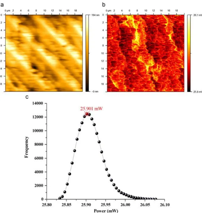
• The maps (Fig 3a–c): the scanning thermal microscope is also an AFM [62] and [63]. Thus, in addition to the classical topographic views (Fig 3a), the SThM can simultaneously draw a thermal contrast map (Fig 3b) revealing the variation of the local thermal conductivity. Hence, this latter displays the power level necessary to keep the surface temperature constant. Thus, as in the roughness analysis for the topographical maps, statistical thermal parameters—like the thermal power distribution curve can be plotted from these latter maps (Fig 3c). After an accurate calibration, we will use this approach for determining the relationship between the contact temperature and the power dissipated on the microscale.

Fig. 2. : SThM curves: (a) μDTA plot: dissipated power vs. contact temperature and (b) μTMA plot: cantilever displacement vs. contact temperature.

Fig. 3. : SThM maps at 300 °C: (a) the topographic view (height contrast) and (b) the thermal contrast map revealing the variation of the local thermal conductivity; (c) the corresponding thermal power distribution curve given the mean value and the standard deviation.

The relationship between the real tribocontact and the SThM tip is schematised in the Fig. 4: the macro-scale tribocontact can be modelled by many micro-asperities at the micro-scale level and connected to the surface roughness (Fig 4a). The real contact area appears to be the sum of the micro-contact areas. Hence, the SThM probe properly simulates the thermal dissipation at the local micro-asperity [27] and [48]. Let us see the various components of the thermal dissipation of the SThM probe as reported by [76], [77] , [78] and [79] and displayed on the Fig. 4b: the initial power Pel injected into the thermoresistance is divided in three

components: the conduction within the wire Qw, the convection in air Qconv (about 6% Pel) and

the heat transfer to the sample Qs. This latter can be also decomposed in the:

• conduction in air Q1=Qcond/air (≅2.5×10−6 WK−1);

• solid–solid conduction Q3=Qsol/sol (depending on K);

• radiation Qrad (negligible).

Fig. 4. : Relationship between the real tribocontact and SThM tip: (a) the tribocontact has many micro-asperities connected to the surface roughness; (b) each asperity is like the SThM tip where the various dissipative components can be identified.

Thus, it clearly appears that the dissipative components (Qconv, Q1, Q2, Q3) reported for the

SThM tip will be also present on the macro-scale distributed on each micro-asperity [45] and [80]. Hence, it is not necessary to dissociate each component of Qs: we assume Qs=Pel−Qconv

where Qconv can be assessed for each temperature when the tip is in the air (Section 3.4).

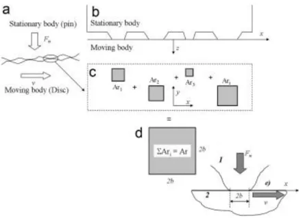
The thermal macrocontact model is described in Fig 5 as a simplification of the Vick et al.'s model [23], [24] and [25] in order to demonstrate the feasibility of our approach. Thus we suppose that the macrocontact is constituted from small square areas Ari (Fig. 5b and c). The

sum of these latter is equal to the real contact area Ar (Fig. 5d). Our goal is to extract the value

of Ar by combining the SThM approach and relation (1). Thus, it should be possible to use the

above surface conjunction temperature theory with the real contact area Ar instead of the

nominal contact area Aa as it is usually done (Fig 5e). In order to accurately estimate the

expected real contact area Ar, we can assume in first approximation that each junction is in a

state of incipient plastic flow. Thus with H=7.8 GPa for our materials (see Section 3.1). This area corresponds to a square (Fig 5d) of about 30 μm×30 μm which is in the same order of magnitude than a SThM image size (Fig 3b). Thus, thermal results of the SThM tests should be significant compared to the thermal phenomena observed on the scale of the macrocontact. Of course, in our approach the crucial point is the calibration of the SThM [54], [55], [56], [74] and [75] . It will be detailed in Section 3.

Fig. 5. : Model of the thermal macro-contact.

In summary:

• Since most of the frictional energy is dissipated as heat, the thermal dissipated power can be determined from the tribological tests by:

(3)Pthermal≈0.95Pfriction≈0.95·μFnv

• The relationship between (i) the thermal dissipated power and the mean/max surface temperature and (ii) the thermal properties of the third body can be assessed using a SThM from the thermal maps established for each temperature.

• The relationship between the real contact area (Ar) and the mean/max surfacetemperature

Tf can be computed using relation (1) with the suitable expression of f determined as a

functional of the Peclet number L.

3. Experimental details

3.1. Samples

Classical metallic samples are not really suitable for this application because they generate plastic flows in addition to the formation of third body—both simultaneously modifying the real contact area. Besides, their high thermal conductivities generate severe distortions of the contact temperature through a time-dependent heat flow. In our case, we need to use

refractory and fragile materials in order to create a third body easily quantifiable with very low thermal diffusivities. Samples are made of sheet nacre extracted from giant oyster

Pinctada maxima currently used for bioprosthetic applications [22] and [27]. This is a natural nanocomposite which has a multiscale structure including a mineral phase of calcium

by an arrangement of CaCO3 biocrystal nanograins (40 nm in size) drowned in an

―intracrystalline‖ organic matrix (4 nm thick) in order to form a microsized flat organomineral aragonite platelet. These platelets are themselves surrounded by an ―intercrystalline‖ organic matrix (40 nm thick) building up a very tough material (E: 54.42±3.27 GPa, ν: 0.25±0.03 and H: 7.82±0.95 GPa [82]). Samples are polished more or less parallel to the aragonite platelets (size: 5 μm, thickness: 400 nm, Ra: 14.5±0.6 nm) (Fig. 1c).

Thermal behaviour of sheet nacre was recently studied by Bourrat et al. [83]. They demonstrated that this material displays some characteristic thermal points allowing us to adjust the relationship between the dissipated thermal power and the surface temperature. In particular, they have shown that:

• The organic matrices begin their degradation process around 250 °C. This “melting process” generates sensor jumps on the μTMA curves (Fig 2b);

• A phase transformation from aragonite to calcite occurs just above 470°C. This phase transformation can be observed by using X-ray diffraction or cathodoluminescence [27]. According to [80] and [84] , density ρ, thermal conductivity K and specific heat σ of nacre are respectively 1850 kg m−3, 3–6 W m−1 K−1 and 1050±150 J kg−1 K−1. K is not very accurate because its value strongly varies with the orientation of the aragonite platelets [83]. Hence, we will determine its value (and the one of the third body) with the SThM using a specific procedure detailed in Section 3.4.

3.2. Tribological tests

The experimental device is a pin-on-disc tribotester manufactured by CSM Instruments (Peseux, Switzerland) [22], [27] and [82]. Tests are carried out at ambient air and room temperature in dry conditions by repeated friction of a 3.5 mm square shaped pin of nacre against the surface of a polished disc of nacre (∅44 mm) (Fig 1a). The normal load (Fn) varies

from 1 to 15 N (i.e. a mean contact pressure lying between 0.1 and 1.2 MPa). The sliding speed and length are respectively 10 mm s−1 and 100 m.

Note that the SThM measurements described below allowing the assessment of the real contact area are not made in-situ on the tribometer. When the steady state of the friction coefficient is observed the sample is removed and placed beneath the SThM in order to evaluate the thermal properties of the third body generated during the test. Thus, in our case, the real contact area actually evaluated is the one which was involved when the test was stopped—i.e. for 100 m of sliding. However, the evolutions of the ―dynamic‖ real contact area could be easily determined using discontinuous tribological tests.

3.3. Atomic force microscopy

Topography of the friction track is assessed using an AFM Dimension 3000 connected to a Nanoscope IIIa electronic controller (Veeco Digital Instruments, Santa Barbara USA) [22] and [81]. Its spatial and vertical resolutions are lower than 1 nm and the field depth is in-between 100 nm and 100 μm. Maps were achieved at high resolution (512×512 pixels) using an intermittent contact mode (so-called TappingMode™). The silicon nitride probe displays a tip rounding lower than 10 nm. The cantilever work frequency, the stiffness and amplitude are respectively: 270 kHz, 42 N m−1 and 25 nm. Depending on the size of the images (between 0.25 and 25 μm2) the scanning rates varies from 1 to 2.4 μm s−1.

AFM views of both the sample and the third body after 100 m of sliding will be used for the validation of the real contact area computation using the ABAQUS finite element code. Image analysis and topographical calculations are made using the SPM software Gwyddion

(http://gwyddion.net) and Scilab 5 (http://scilabsoft.inria.fr).

3.4. Scanning thermal microscopy

The local thermal properties of the samples are assessed with a SThM (TA Instruments μTA 2990 with a TA Instruments controller TA 5300, New Castle, DE) which is an analytical system that combines the high resolution visualization and positioning methods of scanning probe microscopy with the technology of thermal analysis [e.g. 48]. The standard AFM probe is replaced by a thermal probe made from a Wollaston wire (5 μm diameter platinum-10% rhodium wire enclosed in a silver sheath) which allows the acquisition of the surface contact area temperature, and simultaneously acts as a highly localized heater [48], [49], [50], [51], [52] and [53]. The vertical deflection of the assembly is monitored by a light pointing technique. The spring constant is 10 N m−1. The constant current setpoint and the z-setpoint are respectively 1 mA and 50 V. The probe rate is 100 μm s−1. This latter is sufficiently weak so that the heat transfer regime stays in the steady state conduction as in the tribological tests [52] and [64]. The spatial resolution and the thermal sensitivity are respectively about 100 nm and 1 °C [52]:

• Calibration of SThM—connecting the dissipated power with the surface temperature—is made using three reference polymeric samples: PAI TORLON (Tg=285 °C), PEI ULTEM1000

(Tg=215 °C), PPS (Tg=94.4 °C, Tf=281 °C) [27] and [74] .

• Thermal conductivities of the samples (nacre and third body) are determined using the procedure proposed by Ruiz et al. [54] suitable when the sample's conductivity is weak enough. This approach is based to the difference of dissipated flows when the tip is or is not in contact with the sample: Thus Qair is the heat flow rate into the tip when the tip is in

the air (i.e. corresponding to our “zero point”), and Qs=Pel−Qair is the heat flow going into

the sample when the tip is in contact. Qs is evaluated for various reference samples using

the same tip and operating conditions (same topography and ). The error bars are estimated at about 2–3% [54].

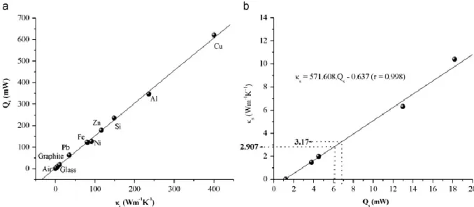
In Fig 6a, Qs=Pel−Qair is plotted as a function of κs for various materials whose thermal

conductivities are accurately known [84]. A linear least-squares fit can be plotted to deduce the thermal conductivity of the unknown samples knowing their respective Qs obtained by the

SThM mean. The enlargement of the Fig. 6b gives respectively 3.17±0.1 W m−1 K−1 for sheet nacre and 2.9±0.09 W m−1 K−1 for the third body. Note that the conductivity of the third body is very close to the one of the sheet nacre because it is formed by the same elemental

biocrystals of CaCO3[22] and [82]. The difference is attributed to a worse organisation of

Fig. 6. : SThM calibration for determining the samples thermal conductivity (a)

determination of the slope given Qs=f(κs) for various reference materials at ΔT=75 °C; (b)

assessment of the conductivity of the sheet nacre (3.17 Wm−1 K−1) and third body (2.907 W m−1K−1).

4. Results and discussion

4.1. Tribological behaviour

Fig. 7a shows the variations of the dissipated power by friction as a function of the sliding length for various normal loads computed from the evolution of the friction force—i.e. Pfriction=Ftv[68]. These curves reveal the existence of a given run-in period probably

associated with the geometric adaptation of the surfaces. Note that the dissipated power varies from 6.2 to 58 mW. Fig. 7b reports the corresponding real coefficient of friction determined after the run-in period by the slope Ft=f(Fn): 0.44±0.02. Thus, despite the structural

complexity of this couple of materials, the quite straight line reveals that their friction

behaviour seems to follow a classical Amontons–Coulomb's law. This latter is often explained by a linear relationship between the normal load (Fn) and the real contact area (Ar) [1], [2],

[8], [9] and [66]. Since 95% of the friction dissipated power is lost by the thermal way [e.g. 69]—the thermal power dissipated at the real contact area level is easily extracted from Fig 7a using relation (3).

Fig. 7. : (a) Variations of the dissipated power by friction vs. sliding length for various normal loads; (b) determination of the corresponding coefficient of friction.

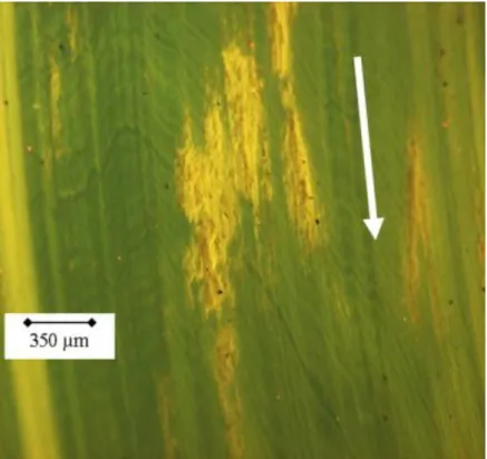
Figure 8 shows typical optical (a) and topographical (b) views of the friction track after 100 m of sliding. The track is partially covered by a third body whose elemental components have the size of the initial aragonite platelets components [22]. Although this third body was already studied in details [22], [27] and [82], it is important to note that the contact is probably made exclusively on this latter. This would explain, on the one hand, the run-in period connected to the set up of a tribolayer within the contact, and on the other hand, the perfect Amontons–Coulomb's behaviour observed after the tribolayer was built. Hence, the thermal power generated during the friction tests would be mainly dissipated through the third body as shown in Fig. 9 displaying the friction track as observed in cathodoluminescence. This technique is particularly sensitive to any modification of the crystal lattice. Thus, for the calcium carbonate, the aragonite structure (orthorhombic lattice) emits in the blue/green whereas the calcite (rhombohedric lattice) emits in the yellow. Hence, Fig. 9 reveals that the third body is mainly constituted by calcite in contrast to the uncovered parts of the friction track. Referring to the work of Bourrat et al. [83], the temperature of the aragonite-calcite phase transformation is generally close to 470 °C. Thus within our tribocontact, these high temperatures can be briefly reached at the level of the microscopic asperities because the thermal conductivities of our samples are very low. Consequently, knowing the thermal power dissipated during the tribological tests, SThM should allow us to determine the temperature levels which can be reached at the interface

Fig. 9. : Typical cathodoluminescence view of the friction track. Aragonite appears in green (dark zone) whereas calcite appears in yellow (bright zone). (For interpretation of the references to colour in this figure legend, the reader is referred to the web version of this article.)

4.2. Thermal behaviour of the third body after 100 m of sliding

SThM is used to link the surface temperature record with the thermal power dissipated at the micro-asperity level. During the imaging process the tip is in direct contact with surfaces. Changes in thermal conductivity across the surface result in a different heat flow in-between the tip and the sample. Hence, changes in this property can be acquired by measuring the power level which is necessary to maintain the tip-temperature at a constant value (Fig. 3b). Fig. 10 reports the evolution of the power level as a function of the contact temperature. The power's value is the average calculated from the thermal power distribution histogram (Fig 3c) extracted from each thermal map (Fig. 3b). This value corresponds to an average on 128×128=16 384 pixels. Error bars refer to the corresponding standard deviations. A linear relationship—with a good correlation coefficient—is clearly observed. Hence a linear fit allows us to connect the thermal power level which is necessary to maintain the mean surface temperature at a constant value. Note that this relationship is no longer linear when the temperature is less than 100 °C (see the μDTA curve in Fig 2a)—i.e. when the dissipated power is less than 5 mW. For these temperature levels the meniscus effect due to the adsorbed water on the sample is no longer negligible. Since the lowest thermal power dissipated during the friction tests is about 5.8 mW (corresponding to 2N in the Fig 7a), it is possible to refine the fit by considering only the values of temperature higher than 100 °C in order to avoid the meniscus effect. Finally the relationship given the surface temperature as a function of the thermal power dissipated during the tribological tests

is:(4)Tf(∘C)=9.1286·Pthermal(mW)+58.521According to the relations (3) and (4), Tf varies

contacts by using embedded thermocouples in the block specimen. In addition the combination of the relations (3) and (4) is in agreement with our previous results on the thermal-induced wear of sheet nacre [27], namely:

• that the minimum dissipated power by friction which is needed to degrade the organic matrix is about 24.5 mW corresponding to a loading of 6N;

• that the aragonite-calcite phase transformation can occur within the contact when the load rises above 11N as shown in the Fig. 9.

Fig. 10. : Variations of the dissipated power vs. the contact temperature as measured by SThM.

4.3. Determination of the real contact area after 100 m of sliding

As mentioned previously we use the simplest model described in the surface conjunction temperature theory—i.e. the square contact (Fig 5e). However, it is possible to use a more complicated thermal model [86], [23] and [24]. All the algebraic equations developed for each surface velocity and contact geometries are available in [64]. Due to the sliding velocity and the pin-on-disc configuration of our tribological tests, one surface (the disc) moves relatively fast with respect to the other (the pin) and a slowly moving heat source model is assumed— i.e. 10 mm s−1 and L≅5. Hence the pin contact temperature stays constant in contrast to the one of the disc which undergoes a thermal cycling. Under the pin, the classical assumptions are [64]:

• Thermal properties of the contacting bodies are independent of the temperature. However, using the above calibration procedure (Section 3.4) the conductivity could be

determined for various ΔT.

• The single area of contact is regarded as a plane source of heat which is given by the SThM power maps (see Fig 3b).

• frictional heat is uniformly generated at the area of contact (Fig 3b and c). • all heat produced is transmitted into the contacting solids via the third body.

The set of equations—giving respectively the average and the maximum flash temperature for the square contact (when b is the half width of the contact and L≅5) is reported below in function of the power dissipated by friction[64]:

(5)

(6)

(7) Ar=4b2K

and χ are respectively the thermal conductivity and the thermal diffusivity of the sample. The constants C1=4.8 and C2=7.9 are extracted for L≅5 from a specific diagram available in [64].

Hence Tfmax is more than 1.6 times Tfmean. Combining the relations (5), (6) and (7) with (4), the

respective real contact areas—computed with the assumption that the SThM thermal measure is either the mean flash temperature(5) or the maximum flash temperature(6)—can be

determined from the knowledge of Pfriction extracted from Fig. 7a. These contact area can be

then compared with the one provided by the classical Greenwood Williamson model (GW). We just point out that the latter requires the knowledge of the involved deformation regime— determined from the AFM topography and the mechanical properties of the samples—thanks to the plastic index Ψ[3]. Thus, in our case:

(8)

where R is the mean radius curvature of the asperity summits (3.96 μm), σ is the standard deviation of summit heights (11.67 nm) and E*, the reduced young modulus (65 GPa). Since the plastic index reveals a prominent elastic behaviour (ψ<0.6) the GW real contact area is then computed with the relation given by [1] and [3]:

(9)

Fig. 11 compares the evolution of the normalised real contact area Ar/Aa as a function of the

normal load for the various models. As expected the elastic GW model follows a classical linear relationship with respect to the normal load in contrast to the thermal models. Although the GW model seems to keep away enough from the thermal ones this discrepancy is not really critical if we look at the one observed between the thermal models which is only due to the difference between Tfmax and Tfmean. In any case, the normalised real contact areas display

Fig. 11. : Variations of the normalised real contact area vs. normal load as respectively computed with the thermal model and the Greenwood Williamson elastic model (Ψ=0.45). In spite of this, the GW model is known to be quite sensitive to the profilometric assessment and, in addition, it does not take into account the presence of third body in contrast to the thermal approach which integrates its effect via the power dissipated by friction. In order to avoid these drawbacks, our thermal model is also confronted to a set of finite element models. The meshes of those models are built from real AFM maps assessed respectively before sliding (1st body, size 2 μm×2 μm) and after 100 m of sliding in presence of third body (size 1 μm×1 μm).

4.4. Validation of the procedure with a finite element code

Basically, an AFM topographic map (Fig 12a) is an array of height data which can be converted to a finite element mesh suitable for numerical simulations (Fig 12b). For this purpose a specific routine was developed from the DynELA FEM library created in C++ language by Pantalé [87]. In order to limit the number of nodes and elements of the mesh, the original resolution of the AFM maps is decreased from 512×512 to 128×128 pixels. From an AFM map the C++ routine generates a meshed surface constituted by 64516 C3D8 elements (127×127×4). The opposite surface is generated from the same AFM image after a 90° rotation and a mirroring operation. Therefore the final numerical model contains 129032 C3D8 elements and 163840 nodes. Then, the two meshed surfaces are brought into contact— with an increasing normal load—by using the ABAQUS FEM Code [88] as schematised in the Fig 12c. The mechanical properties used in the simulations are extracted from [82]. Boundary conditions have also been applied on top and bottom surfaces of the model. All nodes located on bottom surface have a prescribed displacement of zero, while a vertical displacement with an increment of 0.5 nm have been prescribed for all nodes located on the top surface. The real contact area is computed for each loading increment from the number of nodes actually in contact. With this finite element approach, it is also possible to compare the real contact areas in presence or absence of third body using respectively AFM maps of the virgin surface (Fig. 13a) and AFM maps of the friction track observed after 100 m of sliding

(Fig. 13b). In this latter case, the mechanical properties of the third body are evaluated using an inverse method combining nanoindentation and numerical simulations [89].

Fig. 12. : Description of the mesh construction from an AFM map: an original AFM view (a) is transformed in a FEM mesh (b) using a specific C++ routine; The meshed surfaces are brought into contact with an increasing normal load F;(c) the apparent contact is Aa=XY and

the true real contact area is computed from the number of nodes actually in contact Ar=∑Ari

Fig. 13. : von Mises contourplot revealing the growth of the real contact area due to an increasing normal load (a) in absence of third body (1st body before sliding) and (b) in presence of third body (after 100 m of sliding).

Fig. 14 plots the evolution of the normalised real contact area as a function of the normal load for respectively (i) the thermal models, (ii) the elastic GW model and, (iii) the FE models in presence or not of third body. As shown for the GW model, the FE models also follow a linear relationships vs. normal load even in presence of third body (r=0.987). This is in good agreement with respectively the results reported by Myshkin et al. using AFM maps [12] and the perfect Amontons–Coulomb's

behaviour observed in the Section 4.1. Note that the slope of the GW model is noticeably similar (<1%) to the one of the FEM model computed in absence of third body (FEM 1st body) and really greater than the one in presence of the third body (FEM 3rd body). This confirms that the GW model is probably too sensitive to the topography to be really suitable in presence of third body which

continuously changes the topography of the friction track. Although non linear, our thermal models are nearly always included in-between the two finite element models. By comparing the real contact areas obtained respectively using (5) and (6), we find that the best choice is the one obtained when we suppose that the interface temperature is the maximum flash temperature Tfmax. (i.e. the maximum

friction-induced temperature on the tips of interacting asperities materials). Indeed this latter is very close to the FEM model which takes into account the presence of third body. Hence, the thermal model seems to be accurate enough for easily estimating the real contact area in presence of third body. Indeed this thermal approach correctly integrates the influence of the third body through the frictional dissipated power. Of course more complex thermal models should be better for modelling the linear evolution of the real contact area with the normal load.

Fig. 14. : Variations of the normalised real contact area vs. normal load as computed with the Greenwood Williamson elastic model (Ψ<0.45), the thermal models and the FE models in presence and absence of third body.

Fig. 15. : Variations of the real contact pressure vs. normal load as computed with the thermal models and the FE model in presence and absence of third body.

5. Conclusion

In this paper we have described an experimental procedure enabling to estimate the real contact area from the operating parameters (Fn, v, T) and the tribological responses in

presence of third body. A scanning thermal microscope is used for determining (i) the thermal conductivity of both the sample and the third body and, (ii) the relation between the contact temperature and the thermal power dissipated within the interface at the micro-asperity level. These results have been combined with a thermal model commonly used for computing the mean/max surface temperature values—in order to evaluate the real contact area as a function of both the tribological parameters and the heat transfer regime involved during the tests. Results are confronted with both the classical elastic Greenwood Williamson model and ABAQUS finite element models built from the real AFM maps in order to take into account the presence of third body. Results have shown that:

• SThM is a suitable tool for accurately determining the conductivity of complex third body and the surface temperature with respect to the dissipated power.

• the real contact area computed with the thermal method can be really close to the one provided by the FE method in the presence of third body if we suppose that the interface temperature is the maximum flash temperature Tfmax—corresponding to the

maximum friction-induced temperature of the tips of interacting asperities. Besides, the evolutions of the real contact area can be easily determined for various sliding lengths using discontinuous tribological tests. Thus, this approach provides a very simple method enabling to estimate the dynamic real contact area and the

corresponding real contact pressure under tribological solicitations.

• The knowledge of the real contact pressure improves our understanding of the elemental wear mechanisms on the nanoscale. Hence, this experimental approach could be used for studying the wear nanomechanims involving refractory materials in MEMS design (Si3N4, SiC, Al2O3…).

Acknowledgments

The authors are grateful to professor E. Lopez (Museum National d’Histoire Naturelle, Paris) and Dr M. Rousseau (Nancy University, Nancy) for their support and their good advices.

References

[1] C.M. Mate, Tribology on the small scale, Oxford University Press, NY (2008), 333p. [2] F.P. Bowden and D. Tabor, The friction and lubrication of solids, Clarendon Press, Oxford University Press, Oxford, UK (1986).

[3] J.A. Greenwood and J.B.P. Williamson, Contact of nominally flat surfaces. Proc R Soc London, A295 (1966), pp. 300–319.

[4] D.J. Whitehouse and J.F. Archard, The properties of random surfaces of significance in their contact. Proc R Soc London A, 316 (1970), pp. 97–121.

[5] D.J. Whitehouse and J.F. Archard, The contact surfaces having a random structure. J Phys D: Appl Phys, 6 (1973), pp. 289–304.

[6] K.L. Johnson, Contact mechanics, Cambridge University Press (1987), 452p.

[7] J. McCool, Comparison of models for the contact of rough surfaces. Wear, 107 (1986), pp. 37–60.

[8] K.C. Ludema, Friction, wear, lubrication, a textbook in tribology, CRC Press (1996), 257p.

[9] B.N.J. Persson, Sliding friction, physical principles and application, (2nd ed), Springer-Verlag, Berlin Heidelberg (2000), 511p.

[10] H.J. Hertz, On the contact of elastic solids. Reine Angew Math, 92 (1882), p. 156 [11] R.D. Mindlin, Compliance of elastic bodies in contact. J Appl Mech, 71 (1949), pp. 259–268.

[12] Myshkin NK, Kovalev A., Scharff W., Ignatiev M. The effect of adhesion on sliding friction at nanoscale. In: Bartz J., Franek F, editors. Proceedings of the third Vienna

international conference NANO-TECHNOLOGY, 2009. p. 323–7, ISBN 978-3-901657-32-0..

[13] A. Tudor and L. Seiciu, An elastic–plastic model with adhesion for the sphere-flat contact, D. Dowson, Editor, et al.The third body concept, Elsevier Science B.V. (1996), pp. 675–681.

[14] K.L. Johnson, K. Kendall and D. Roberts, Surface energy and contact of elastic solids. Proc R Soc London, A324 (1971), p. 301.

[15] B.V. Derjarguin, V.M. Muller and Y.P.T. Toporov, Effect of contact deformation on adhesion of particles. J Colloid Interface Sci, 53 (1975), p. 314.

[16] T.R. Thomas, Rough surfaces, (2nd ed), Imperial College Press (1999), 278p.

[17] N.K. Myshkin, S.A. Chizhik and V.V. Gorbunov, Nanoscale topography and tribological problems. Tribol Int, 28 1 (1995), pp. 39–43.

[18] J.A. Greenwood, Problems with surface roughness, I.L. Singer, H.M. Pollock, Editors , Fundamentals of friction: macroscopic and microscopic processes, Kluwer, Dordrecht, NL (1992), pp. 57–76.

[19] M. Brendlé, P. Diss and P.H. Stempflé, Nanoparticle detachment: a possible link between macro- and nanotribology. Tribol Lett, 9 (2000), pp. 97–104.

[20] P.H. Stempflé, G. Castelein and M. Brendlé, Influence of environment on the size of the elemental wear debris of graphite, D. Dowson, Editor, et al.Boundary and mixed lubrication: science and applications, Elsevier Science (2002), pp. 295–304.

[21] R. Colaço, Surface-damage mechanisms: from nano- and microcontacts to wear of materials, E. Gnecco, E. Meyer, Editors , Fundamentals of fiction and wear on the nanoscale, Springer-Verlag, Berlin, Heidelberg (2007) ISBN: 13 978-3-540-36806-9.

[22] P.H. Stempflé and M. Brendlé, Tribological behaviour of nacre—influence of the environment on the elementary wear processes. Tribol Int, 39 (2006), pp. 1485–1496. [23] B. Vick, M.J. Furey and K. Iskandar, Theoretical surface temperatures generated from sliding contact of pure metallic elements. Tribol Int, 33 (2000), pp. 265–271.

[24] B. Vick and M.J. Furey, A basic theoretical study of the temperature rise in sliding contact with multiple contacts. Tribol Int, 34 (2001), pp. 823–829.

[25] B. Vick and M.J. Furey, An investigation into the influence of frictionally generated surface temperatures on thermionic emission. Wear, 254 (2003), pp. 1155–1161. [26] M.J. Furey, B. Vick, H.M.R. Ghasemi and J.H. Bohn, Coalescence and breakup of temperature areas: effects on surface temperatures. Tribol Int, 40 (2007), pp. 595–600. [27] P.H. Stempflé, T. Djilali, R. Kouitat Njiwa, M. Rousseau, E. Lopez and X. Bourrat, Thermal-induced wear mechanisms of sheet nacre in dry friction. Tribol Lett, 35 (2009), pp. 97–104.

[28] J.A. Greenwood and J.M. Tripp, The elastic contact of rough spheres. Trans ASME J Appl Mech, 12 (1967), pp. 153–159.

[29] P.R. Nayak, Random process model of rough surfaces. ASME J Lubr Technol, 93 (1971), p. 398.

[30] B. Bhushan, Contact mechanics of rough surfaces in tribology: multiple asperity contact. Tribol Lett, 4 (1998), pp. 1–35.

[31] B.N.J. Persson, O. Albohr, U. Tartaglino, A.I. Volokitin and E. Tosatti, On the nature of surface roughness with application to contact mechanics, sealing, rubber friction and

adhesion. J Phys: Condens Matter, 17 (2005), pp. R1–R62.

[32] H. Zahouani and F. Sidoroff, Rough surfaces and elasto-plastic contacts. C.R. Acad Sci Paris, t.2 IV (2001), pp. 709–715.

[33] A. Majumdar and B. Bhushan, Fractal model of elastic–plastic contact between rough surfaces. J Tribol-Trans ASME, 113 (1991), p. 1.

[34] A.W. Bush, R.D. Gibson and T.R. Thomas, The elastic contact of rough surface. Wear, 35 (1975), pp. 87–111.

[35] W.R. Chang, I. Etsion and D.B.P. Bogy, An elastoplastic model for contact of rough surfaces. ASME J Tribol, 109 (1987), p. 587.

[36] Z. Liu, A. Neville and R.L. Reuben, An analytical solution for elastic and elasto-plastic contact models. Tribol Trans, 43 4 (2000), pp. 627–634.

[37] R.L. Jackson, R.S. Duvvuru, H. Meghani and M. Mahajan, An analysis of elasto-plastic sliding spherical asperity interaction. Wear, 262 (2007), pp. 210–219.

[38] R.L. Jackson and J.L. Streator, A multiscale model for contact between rough surfaces. Wear, 261 (2006), pp. 1337–1347.

[39] F. Robbe-Valloire, B. Paffoni and R. Progri, Load transmission by elastic, elastoplastic or fully plastic deformation of rough surface asperities. Mech Mater, 33 (2001), pp. 617– 633.

[40] J. Jamari and D.J. Schipper, Deformation due to contact between a rough surface and a smooth ball. Wear, 262 (2007), pp. 138–145.

[41] Berthier Y. Background on friction and wear. In: Lemaitre J., editor. Handbook of materials behaviour models failures of materials, vol. 2, 2001. p. 676–99 ISBN 0-12-443341-3..

[42] P.H. Stempflé and J. Von Stebut, Nanomechanical behaviour of the 3rd body generated in dry friction—feedback effect of the 3rd body and influence of the surrounding environment on the tribology of graphite. Wear, 260 (2006), pp. 601–614.

[43] P.H. Stempflé, F. Pollet and L. Carpentier, Influence of intergranular metallic nanoparticles on the fretting wear mechanisms of FeCrAl2O3 nanocomposites rubbing on

Ti6Al4V. Tribol Int, 41 (2008), pp. 1009–1019.

[44] R. Holm, Electrical contacts handbook, Springer-Verlag, H Gerber Pub, Berlin, Stockholm (1946).

[46] Eguchi M, Shibamiya T, Yamamoto. Analysis of area and stick-slip region of real contact using white light interferometry. In: Bartz J, Franek F, editors. Proceedings of the third Vienna international conference on NANO-TECHNOLOGY; 2009. p. 179–86. ISBN 978-3-901657-32-0..

[47] M. Sato, T. Watarai, K. Miyata, T. Inagaki and Y. Okamoto, Study on heat transfer and temperature field of rotating friction interface, D. Dowson, Editor, et al.The third body concept, Elsevier Science (1996), pp. 247–256.

[48] H.M. Pollock and A. Hammiche, Micro-thermal analysis: technique and applications. J Phys D: Appl Phys, 34 (2001), pp. R23–R53.

[49] J. Ye and A. Okada, Micro-thermal analysis for advanced silicon nitrides. J Eur Ceram Soc, 24 (2004), pp. 441–448.

[50] F.A. Guo, N. Trannoy and J. Lu, Analysis of thermal properties by scanning thermal microscopy in nanocrystallized iron surface induced by ultrasonic shot peening. Mater Sci Eng A, 369 (2004), pp. 36–42.

[51] V.V. Tsukruk, V.V. Gorbunov and N. Fuchigami, Microthermal analysis of polymeric materials. Thermochim Acta, 395 (2003), pp. 151–158.

[52] S. Gomes, N. Trannoy, P. Grossel, F. Depasse, C. Bainier and D. Charraut, D.C. scanning thermal microscopy: characterisation and interpretation of the measurement. Int J Therm Sci, 40 (2001), pp. 949–958.

[53] R. Häßler and E. zur Mühlen, An introduction to μTA™ and its application to the study of interfaces. Thermochim Acta, 361 (2000), pp. 113–120.

[54] F. Ruiz, W.D. Sun, F.H. Pollak and C. Venkatraman, Determination of the thermal conductivity of diamond-like nanocomposite films using a scanning thermal microscope. Appl Phys Lett, 73 13 (1998), pp. 1802–1804.

[55] V.V. Gorbunov, N. Fuchigami, J.L. Hazel and V.V. Tsukruk, Probing surface

microthermal properties by scanning thermal microscopy. Langmuir, 15 (1999), pp. 8340– 8343.

[56] S. Lefèvre, S. Volz, J.-B. Saulnier, C. Fuentes and N. Trannoy. Rev Sci Instrum, 74 4 (2003), pp. 2418–2423.

[57] V.M. Asnin, F.H. Pollak, J. Ramer, M. Schurman and I. Ferguson, High spatial

resolution thermal conductivity of lateral epitaxial overgrown GaN/sapphire (0001) using a scanning thermal microscope. Appl Phys Lett, 75 9 (1999), pp. 1240–1242.

[58] G.B.M. Fiege, A. Altes, R. Heiderhoff and L.J. Balk, Quantitative thermal conductivity measurements with nanometre resolution. J Phys D: Appl Phys, 32 (1999), pp. L13–L17. [59] S. Callard, G. Tallarida, A. Borghesi and L. Zanotti, Thermal conductivity of SiO2 films

[60] S. Gomès, L. David, V. Lysenko, A. Descamps, T. Nychyporuk and M. Raynaud,

Application of scanning thermal microscopy for thermal conductivity measurements on meso-porous silicon films. J Phys D: Appl Phys, 40 (2007), pp. 6677–6683.

[61] F.A. Guo, K.Y. Zhu, N. Trannoy and J. Lu, Examination of thermal properties by scanning thermal microscopy in ultrafine-grained pure titanium surface layer produced by surface mechanical attrition treatment. Thermochim Acta, 419 (2004), pp. 239–246. [62] C. Wang, The principle of micro thermal analysis using atomic force microscope. Thermochim Acta, 423 (2004), pp. 89–97.

[63] A. Hammiche, H.M. Pollock, M. Song and D.J. Hourston, Sub-surface imaging by scanning thermal microscopy. Meas Sci Technol, 7 (1996), pp. 142–150.

[64] G.W. Stachowiak and A.W. Batchelor, Engineering tribology, Butterworth-Heinemann Ltd. (2002), 744p.

[65] Myshkin NK, Petrokovets MI, Chizhik SA. Simulation of real contact in tribology. Invited papers, WTC97, London, MEP; 1997. p. 329–37..

[66] P.J. Blau, Friction science and technology, Marcel Dekker, Inc., NY (1996), 399p. [67] A. Ramalho and J.C. Miranda, The relationship between wear and dissipated energy in sliding systems. Wear, 260 (2006), pp. 361–367.

[68] D. Shakhvorostov, K. Pöhlmann and M. Scherge, An energetic approach to friction, wear and temperature. Wear, 257 (2004), pp. 124–130.

[69] R. Gras, Tribologie, Dunod, Paris (2008) 978-2-10-005607-1 .

[70] H. Blok, Theoretical study of temperature rise at surfaces of actual contact under oiliness lubricating conditions, general discussion on lubrication. Inst Mech Eng, London, 2 (1937), pp. 222–235.

[71] H. Blok, The flash temperature concept. Wear, 6 (1963), pp. 483–494.

[72] J.C. Jaeger, Moving sources of heat and the temperature at sliding contacts. Proc R Soc, N.S.W., 76 (1943), pp. 203–224.

[73] J.F. Archard, The temperature of rubbing surfaces. Wear, 2 1958/59 (1958), pp. 438– 455.

[74] μTA 2990 Operator's manual. Calibrating the μTA 2990; 2003. p. 113–29..

[75] Blaine RL, Slough CG, Price DM. Micro thermal analysis calibration, repeatability and reproducibility. In: Proceedings of the 27 conference of the North American thermal analysis society, september 20–22, Savannah, Georgia; 1999. p. 691–96..

[76] L. Shi and A. Majumdar, Thermal transport mechanisms at nanoscale point contacts. J Heat Transfer, 124 (2002), pp. 329–337.

[77] Gomès S, Trannoy N, Grossel P. DC thermal microscopy: study of the thermal exchange between a probe and a sample. Meas Sci Technol 1999;10:805–11..

[78] L. David, S. Gomès and M. Raynaud, Modelling for the thermal characterization of solid materials by DC scanning thermal microscopy. J Phys D: Appl Phys, 40 (2007), pp. 4337– 4346.

[79] F. Depasse, P.H. Grossel and S. Gomès, Theoretical investigations of DC and AC heat diffusion for submicroscopies and nanoscopies. J Phys D: Appl Phys, 36 (2003), pp. 204– 210.

[80] Z.M. Zhang, Nano/microscale heat transfer, NewMcGraw-Hill Nanoscience and Technology Series (2007), 479p.

[81] M. Rousseau, E. Lopez, P.H. Stempflé, M. Brendlé, L. Franke and A. Guette, et al. Multiscale structure of sheet nacre. Biomaterials, 26 31 (2005), pp. 6254–6262.

[82] P.H. Stempflé, O. Pantalé, R. Kouitat Njiwa, M. Rousseau, E. Lopez and X. Bourrat, Friction-induced sheet nacre fracture: effects of nanoshocks on cracks location. Int J Nanotechnol, 4 6 (2007), pp. 712–729.

[83] X. Bourrat, L. Franck, E. Lopez, M. Rousseau, P.H. Stempflé and M. Angellier, et al. Nacre biocrystal thermal behaviour. CrystalEngComm, 9 (2007), pp. 1205–1208.

[84] Brady GS, Clauser HR, Vaccari JA. Materials handbook, 14th ed. McGraw-Hill Companies, 1996. 1136p. ISBN-10:0070070849, ISBN-13:978-0070070844..

[85] J. Takadoum, Materials and surface engineering in tribology, ISTE Ltd Wiley, London (2008), 226p.

[86] J.J. Salgon, F. Robbe-Valloire, J. Blouet and J. Bransier, A mechanical and geometrical approach to thermal contact resistance. Int J Heat Mass Transfer, 40 5 (1997), pp. 1121– 1129.

[87] O. Pantalé, An object-oriented programming of an explicit dynamics code: application to impact simulation, . Adv Eng Software, 33 5 (2002), pp. 275–284 8.

[88] ABAQUS. ABAQUS-standard user manual, Version 6.8. In Hibbit, Karlsson, Sorenson (HKS) Inc (editors). 1997 Rhode Island, USA: Hibbit, Karlsson, Sorenson (HKS) Inc.. [89] P.H. Stempflé and F. Schäfer, Hybrid algorithm for identifying the nanomechanical properties of materials and thin films: application to tribological transfer films. Int J Surf Sci Eng, 1 2/3 (2007), pp. 213–238.

[90] Stempflé PH, Pantalé O, Rousseau M, Lopez E, Bourrat X. Mechanical properties of the elemental nanocomponents of nacre structure, 2010, to be published..