HAL Id: hal-01502637
https://hal-agroparistech.archives-ouvertes.fr/hal-01502637
Submitted on 26 Sep 2017
HAL is a multi-disciplinary open access
archive for the deposit and dissemination of
sci-entific research documents, whether they are
pub-lished or not. The documents may come from
teaching and research institutions in France or
abroad, or from public or private research centers.
L’archive ouverte pluridisciplinaire HAL, est
destinée au dépôt et à la diffusion de documents
scientifiques de niveau recherche, publiés ou non,
émanant des établissements d’enseignement et de
recherche français ou étrangers, des laboratoires
publics ou privés.
Distributed under a Creative Commons Attribution| 4.0 International License
poisson null hypothesis
Eric Marcon, Stephane Traissac, Gabriel Lang
To cite this version:
Eric Marcon, Stephane Traissac, Gabriel Lang. A statistical test for ripley’s K function rejection of
poisson null hypothesis. International Scholarly Research Network, ISRN Ecology, 2013, 2013 (Article
ID753475), 9 p. �10.1155/2013/753475�. �hal-01502637�
Hindawi Publishing Corporation ISRN Ecology
Volume 2013, Article ID 753475,9pages
http://dx.doi.org/10.1155/2013/753475
Research Article
A Statistical Test for Ripley’s
𝐾 Function Rejection of
Poisson Null Hypothesis
Eric Marcon,
1Stéphane Traissac,
1and Gabriel Lang
2,31AgroParisTech, UMR EcoFoG, BP 709, French Guiana, 97310 Kourou, France 2AgroParisTech, UMR 518 Math. Info. Appli., 75005 Paris, France
3INRA, UMR 518 Math. Info. Appli., 75005 Paris, France
Correspondence should be addressed to Eric Marcon; [email protected] Received 10 January 2013; Accepted 14 March 2013
Academic Editors: U. M. Azeiteiro and J.-P. Rossi
Copyright © 2013 Eric Marcon et al. This is an open access article distributed under the Creative Commons Attribution License, which permits unrestricted use, distribution, and reproduction in any medium, provided the original work is properly cited. Ripley’s𝐾 function is the classical tool to characterize the spatial structure of point patterns. It is widely used in vegetation studies. Testing its values against a null hypothesis usually relies on Monte-Carlo simulations since little is known about its distribution. We introduce a statistical test against complete spatial randomness (CSR). The test returns the𝑃 value to reject the null hypothesis of independence between point locations. It is more rigorous and faster than classical Monte-Carlo simulations. We show how to apply it to a tropical forest plot. The necessary R code is provided.
1. Introduction
The commonest tool used to characterize the spatial structure of a point set is Ripley’s 𝐾 statistic [1, 2]. It has been widely used in ecology and other scientific fields and is well referenced in handbooks [3–7]. Classically, an observed set of points is tested against a homogeneous Poisson point process taken as a null model. Since little is known about
the distribution of the𝐾 function, the test of rejection of
the null hypothesis relies on Monte-Carlo simulations. Large point patterns are difficult to deal with because computation time is roughly proportional to the square of the number of points (to calculate the distances between all pairs of points) multiplied by the number of simulations. Moreover, the test is valid for one distance but using it repeatedly for all distances
where the 𝐾 function is calculated dramatically increases
the risk to reject the null hypothesis by error [8]. Duranton
and Overman [9] provided a heuristic global test followed
by Marcon and Puech [10]. Loosmore and Ford proposed a
goodness-of-fit test to eliminate this error, but still rely on Monte-Carlo simulations.
We showed in [11] that a global test was able to return a classical𝑃 value, that is to say, the probability to erroneously reject the null model, relying on exact values of the biases
and variances of the statistics. We derived its asymptotic properties in a growing square window. We develop it in this paper so that it can be used in a rectangular window, as most applications require. We show that it can be applied to real point patterns, even with a little number of points and discuss in depth the way to employ it, so that it can be used by empirical researchers.
We first present our motivating example: a tropical forest plot where we want to elucidate the spatial structure of two species of trees. We provide the mathematical framework supporting the test. We apply it to the dataset and present the results. In the Discussion, we review the literature of previous tests to show why this one is a significant improvement and we verify that the test actually works. Finally, we provide a user guide to allow researchers to easily apply the test with the provided R [12] code.
2. Materials and Methods
2.1. Data to Analyze. We consider the distribution of two tree
species in Paracou field station, French Guiana [13]. All trees over 10 cm DBH have been plotted. We use data from a 400.6 by 522.3 meters rectangle included in the four plots of the
(a) (b)
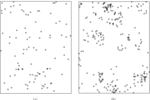
Figure 1: Map of Tachigali melinonii (94 trees, (a)) and Dicorynia guianensis (254 trees, (b)).
southern block of the experimental device. A map of trees is
inFigure 1.
Dicorynia guianensis Amsh. is a widely studied species in
French Guiana; its spatial structure has been characterized for a long time [14,15]; as a visual inspection of the map allows to guess, Dicorynia guianensis is an aggregated species.
Much less is known about Tachigali melinonii (Harms) Barneby. The species has been studied for its special biome-chanical behavior [16] or leaf trait plasticity [17]. The spatial structure of its saplings has been reported by Flores et al. [18] but the structure of adult trees is not clear.
2.2. Mathematical Framework. We consider a point pattern
in a rectangular window.𝑙1and𝑙2are the sides of the window
(width and length). 𝜌 is the intensity of the underlying
point process; estimated by the number of observed points 𝑁 divided by the area of the window. We denote by r the vector of distances(𝑟1, . . . , 𝑟𝑖, . . . , 𝑟𝑑). We omit the subscript
for readability when there is no ambiguity;𝑟 is one of the
distances, and ̂𝐾(𝑟) is the estimator of 𝐾 at distance 𝑟. Points are denoted by𝜉𝑖, and𝐼{𝑑(𝜉𝑖, 𝜉𝑗) ≤ 𝑟} is an indicator function equal to 1 when the distance between two points is less than or equal to𝑟, 0 else. Details of the calculation are not provided as we follow exactly Lang and Marcon [11] but its important steps and intuitions are presented here.
Ripley’s 𝐾 function is estimated from the data for each
distance𝑟, without correction for edge effects: ̂
𝐾 (𝑟) = 𝑙1𝑙2
𝑁 (𝑁 − 1)𝜉𝑖∑̸= 𝜉𝑗𝐼 {𝑑 (𝜉𝑖, 𝜉𝑗) ≤ 𝑟} . (1)
Assumptions are those of Ripley’s 𝐾 function: we test the
independence of locations of an observed point pattern, assumed to be a realization of a homogenous point pro-cess. Homogeneity means both stationarity (the process
in unchanged by translation) and isotropy (the process is unchanged by rotation). Thus the null hypothesis of complete spatial randomness (CSR) is that the point process is a homogenous Poisson process.
The expectation of𝐾(𝑟) under CSR is 𝜋𝑟2. Edge effects
introduce a bias in ̂𝐾(𝑟), computed for the null model: 𝐵 (𝑟) = −4𝑟33𝑙(𝑙1+𝑙2) 1𝑙2 + 𝑟4 2𝑙2 1𝑙22 . (2)
Estimated ̂𝐾(𝑟) can be corrected for the bias of the null model to test them against it. We get a vector of results of length𝑑:
̂
K= (̂𝐾 (𝑟1) − 𝐵 (𝑟1) , ̂𝐾 (𝑟2) − 𝐵 (𝑟2) , . . . , ̂𝐾 (𝑟𝑑) − 𝐵 (𝑟𝑑)) .
(3)
For a homogenous point process the vector ̂K − 𝜋r2 is
asymptotically normal, with expectation zero and the explicit
variance matrixΣ: Σ = ( Var(̂𝐾 (𝑟1)) ⋅ ⋅ ⋅ cov (̂𝐾 (𝑟1) , ̂𝐾 (𝑟𝑑)) .. . d ... cov (̂𝐾 (𝑟1) , ̂𝐾 (𝑟𝑑)) ⋅ ⋅ ⋅ Var(̂𝐾 (𝑟𝑑)) ) . (4) Consequently𝑇2 = ‖Σ−1/2(̂K − 𝜋r2)‖2follows a𝜒2law with 𝑑 degrees of freedom. Asymptotic value of the variance is reached with dozens of thousand points, so it is of little use, but normality is acceptable with very few points so the test
can be used with real data, as the exact value ofΣ can be
calculated. The exact calculation of variance and covariance is quite painful because it takes into account the edge effects, resulting in the formulas given inAppendix A.
ISRN Ecology 3
2.3. Application. The test is applied as follows: (i) compute
̂
K − 𝜋r2from the observed point pattern, following (3); (ii)
computeΣ according to the window’s size and the number of
observed points; (iii) finally compare𝑇2= ‖Σ−1/2(̂K − 𝜋r2)‖2 to a𝜒2distribution with𝑑 degrees of freedom and return the 𝑃 value.
We provide a classical plot of𝐿(𝑟) = √𝐾(𝑟)/𝜋 − 𝑟 [19]
against𝑟, computing every 5 meters up to 250 m (to illustrate the discussion). 1,000 simulations of a binomial process with the same number of points as the real data are run. At each distance𝑟, the 25 lower and greater values are eliminated to build the local 5% confidence interval. The global confidence interval is built iteratively [9,10]; simulations corresponding to extreme values (maximum or minimum) at any distance are eliminated. This process is repeated until 5% of the simulations are concerned. The extreme remaining values are plotted. Interpolation is used if the last iteration eliminates more simulations than required.
We apply our test to these two point sets, up to 150 meters following Collinet [15] who characterized the spatial structure of many species in Paracou and detected possible
dependence at this scale. The vector of distances is r =
(10, 20, . . . , 150) meters; we discuss this choice later. Finally,
we apply Loosmore and Ford’s test based on the samer and
1,000 simulations.
3. Results
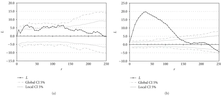
Aggregation of Dicorynia guianensis is obvious on
Figure 2(b). Our test applied with the vector of distances (10,
20,. . ., 150 meters) returns a 𝑃 value equal to zero; that is
to say, the quantile of the 𝜒2 distribution with 15 degrees
of freedom for𝑇 is so low that R returns 0. Loosmore and
Ford’s test gives the same result with a value of their statistic 𝑢1much greater than all simulations.
Figure 2(a)shows a less clear structure of Tachigali
meli-nonii. The curve leaves the local confidence interval many
times, but not the global one. Our test applied with the same distance vector (10 to 150 m) returns a𝑃 value equal to 2.5%; aggregation is significant.
Loosmore and Ford’s test applied to the same distance
range returns a𝑃 value equal to 1.7% ± 0.8% (𝑢1is ranked
984th among the 1,000 simulations).
4. Discussion
4.1. Foundations of the Test. Many methods exist to test a
point pattern against CSR [7, page 83:98], among which the
relative variance [20,21] or tests based on the nearest neigh-bors [22–24]. Tests based on the𝐾 function are particularly appealing because ̂K provides data about the relative position of points at different scales, and the function simultaneously gives useful information about the point process.
4.1.1. The Distribution of ̂𝐾(𝑟) under CSR Was Unknown. The
classical, local test consists in comparing each observed ̂𝐾(𝑟)
to the confidence interval of ̂𝐾(𝑟) obtained by Monte-Carlo
simulations of the null model (which should be a homoge-nous Poisson point process, but is usually approximated by a binomial process for simplicity, artificially reducing vari-ability). The null model is rejected at the chosen significance level, 5%, when the observed ̂𝐾(𝑟) is out of the corresponding confidence interval.
To avoid simulations, approximate confidence intervals for ̂𝐾(𝑟) were proposed by Ripley [25], refuted by Koen [26] whose errors were finally corrected by Chiu [27]. All these confidence intervals were built on simulations.
The variance of ̂𝐾(𝑟) has been investigated early (see [5, page 58]). Asymptotic variance was calculated and asymp-totic normality was proved, allowing calculating a confidence
interval for ̂𝐾(𝑟), but the exact variance remains far from
its asymptotic value for usual point sets [11]. We derived the exact variance inAppendix A.
4.1.2. Testing ̂𝐾(𝑟) along Many Values of 𝑟 Is Not Correct. In
our examples, we have 30 values of ̂𝐾(𝑟). If we draw a point pattern in a Poisson process we can expect 5% of them, that is, 1 or 2 of them, to be out of the confidence interval. As a consequence, the local significance level of the test should be decreased dramatically to have a global significance level
of 5%. Actually, ̂𝐾(𝑟) are highly correlated because 𝐾 is a
cumulative function; roughly speaking, most of ̂𝐾(𝑟) values
come from that of the previous one (see Figure 3). This
reduces the need for a correction but does not eliminate it
completely [28]. Since no quantification of the correction
is available, the local test is used, keeping in mind that the global significance level of the test is somehow higher than announced (see [7, page 456] for a discussion). Each of the local confidence interval values is correct but testing a curve made of 30 points against local confidence envelope is not [8]. To address this issue, solutions have been proposed.
Duranton and Overman [9] proposed a test consisting in
eliminating simulated ̂K vectors globally when one of their
values is an extreme one. Global confidence intervals plotted in the figures are heuristic; they do not rely on any mathemat-ical proof. They appear to be too conservative for Tachigali
melinonii.
4.1.3. Goodness-of-Fit Tests Are a Solution. Goodness-of-fit
(GoF) tests measure the discrepancy between the expected
curve of𝐾 under the null hypothesis and the actual curve.
This value can be compared to its quantiles under CSR. Loosmore and Ford’s [8] test is a GoF test, already proposed by Diggle [4]. Its quantiles are not known so the test relies on Monte-Carlo simulations. Three GoF tests have been proposed by Heinrich [29] but all of them are asymptotic so none can be used with real data. Our test is very similar to Heinrich’s𝜒2test, but as we derived the bias due to edge effects and the exact variance-covariance matrix of ̂K under CSR, we were able to compute the𝑇2statistic, which follows an𝜒2law whose quantiles are well known.
4.1.4. Graphical Interpretation of the Test. Figure 3(a)shows
𝑟 0 50 100 150 200 250 𝐿 20.0 15.0 10.0 5.0 0.0 −5.0 −10.0 −15.0 𝐿 Global CI 5% Local CI 5% (a) 𝐿 Global CI 5% Local CI 5% 𝑟 0 50 100 150 200 250 𝐿 25.0 20.0 15.0 10.0 5.0 0.0 −5.0 −10.0 (b)
Figure 2:𝐿 values for Tachigali melinonii (a) and Dicorynia guianensis (b). Distances are in meters. Confidence intervals are computed for the null hypothesis of complete spatial randomness at the 5% significance level. The local [4] and global [9] confidence intervals are calculated by Monte-Carlo simulations as explained in the text. Test𝑃 values are respectively 0 and 2.5%.
0.8 0.6 0.4 0.2 0.0 −0.2 −0.4 −0.6 4 3 2 1 0 −1 −2 −3 𝐾(2) − 𝐸(𝐾(2)) 𝐾 (2) − 𝐸(𝐾(2)) (a) 𝑇(2) 3 2 1 0 −1 −2 −3 𝑇( 5) 2 1 0 −1 −2 −3 (b)
Figure 3: (a) Plot of ̂𝐾 minus its expectation 𝜋𝑟2in two dimensions (𝑟 = 2 and 𝑟 = 5) for 500 simulations of a Poisson process of intensity 𝜌 = 5 drawn in a square window of size 10 (500 points on average). (b) Comparison of values of 𝑇(2) and 𝑇(5), after transformation. Around 25 simulations of the homogenous point process out of 500 lie out of the critical circle corresponding to𝑇2> 𝜒5%2 (2) so they are rejected by the test.
of𝑟. Each point represents a simulation of a Poisson process.
The plot should be imagined in a number of dimensions𝑑
equal to the number of𝑟 values. As 𝐾 is a cumulative function, its values are highly autocorrelated.Figure 3(a)presents the results of simulations of a Poisson point process. Some are slightly aggregated (positive values); others are dispersed
(negative values) due to stochasticity. Multiplying byΣ−1/2 yields values of T = Σ−1/2(̂K − 𝜋r2) that are independent, centered, and of variance 1 (Figure 3(b)). We denote by𝑇(𝑟)
each element ofT and 𝑇 = ‖T‖.
The circle’s radius is the square root of the 5% critical value of an𝜒2distribution with 2 degrees of freedom. Point patterns
ISRN Ecology 5
Table 1: Number of rejections of the null hypothesis (the point process is Poisson) out of 10,000 simulations of a homogenous point process in a rectangular 10 by 15 window. The significance level is 5%, so 500 simulations are expected to be rejected. The intensity varies from 1/3 to 10 so that the expected number of points varies from 50 to 1500, covering the range of usually-studied point patterns.
Expected number of points 50 100 150 300 750 1500 Number of rejections 592 587 543 537 524 543
corresponding to plots outside the circle are rejected. Thus, the test detects significant regularity of points (example not shown) as well as aggregation.
Transforming correlated ̂K values into independent T
whose squared norm follows an𝜒2distribution relies on the
exact, not asymptotic, variance matrix.
4.1.5. Correcting Edge Effects for the Null Model Is a Better Choice. Classically, edge effects are corrected when
estimat-ing𝐾. Corrections assume unseen neighbors exist beyond
the window’s limits and evaluate their number according to observed data inside the window. We prefer to calculate the bias of the null model and compare empirical, uncorrected values of𝐾 to their expected, biased values; see (3). We follow
Gignoux et al. [24] who showed that testing data against
CSR with nearest-neighbor functions was more powerful when ignoring edge effects (i.e., neither the actual point pattern nor Monte-Carlo simulations of the null hypothesis were corrected). Heuristically, correcting edge effects for each point means adding neighbors uniformly, reducing the power of the test against CSR.
4.2. Test of the Test. Although we use the exact variance
matrix, we only proved asymptotical normality. This is a common issue of statistical tests; the confidence interval of an average value calculated from 30 repeated measures is usually evaluated assuming normality, only asymptotically proved.
We evaluated the minimum number of points necessary to validate the level of the test. We simulated 10,000
realiza-tions of a Poisson point process in a10×15 rectangle window
and tested them. ̂K was calculated at distances 1, 2, 3, 4, and 5. Intensity was chosen between 1/3 and 10, so that the expected number of points ranged between 50 and 1500.
Figure 4shows the actual levels of rejections of the test
(extreme intensities only are shown for readability). When
points are few, the number of simulated patterns whose 𝑇
value is above the critical value of𝜒2at low risk levels (e.g., 1%) is a little more than the risk level. At the 5% risk level, we believe the test results are acceptable for practical purposes even with very few points. We expect 500 simulations to be rejected;Table 1shows the rejection level is always under 6%.
We also wanted to evaluate the power of the test, that is to say, its ability to reject point patterns that are not completely random but hard to detect. Grabarnik and Chiu
[30] proposed to use a mixture of Mat´ern and Strauss
processes as a counterfactual. They tested the ability different
statistics including Ripley’s 𝐾 to distinguish them from a
Poisson process. We followed them to draw a power test
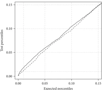
Expected percentiles 0.00 0.05 0.10 0.15 Te st p er cen tiles 0.15 0.10 0.05 0.00
Figure 4: Actual rejection levels versus expected ones: ordinates are the quantiles of simulated Poisson point patterns whose𝑃 values are below the value in abscissa. Curves are built from 10,000 simulations of homogenous Poisson point processes with different intensities (solid line: 50 points expected, dashed line: 1500 points). More simulations are rejected than should be when the number of points is low, but the discrepancy is less than 1%. With 1500 points, the quantiles of the test are very close to their expected values.
presented inAppendix B. Unsurprisingly, we find that our
test’s power is very similar to that of𝐾 in Grabarnik and
Chiu’s tests.
4.3. Choosing the Distance Vector. The choice of𝑟 values (the
vector of distances) is arbitrary. If the point process is actually
a homogenous Poisson, results are identical whatever r is.
Since it may not be, some rules should be followed; choosing the distances up to the expected range of interactions, with uniform steps, allows an “objective” analysis of the data [29], better than selecting values from the plots.
The 𝑇 statistic is the sum of contributions of 𝑇(𝑟) for
all r values. 𝑇(𝑟) are made independent by construction.
Taking into account distances above the maximum range of interaction between points limits the power of the test since a fraction of the𝑇(𝑟) values are purely stochastic. This is a normal behavior for a goodness-of-fit test. When used on the whole distance range 0–250, Loosmore and Ford’s [8] test applied to the Tachigali example loses its power and returns
a𝑃 value equal to 23.5%. In the same conditions, our test
returns a 𝑃 value equal to 6.3%; it appears to lose much
less power when noisy data (there is no interaction between points at such distances) is introduced in the analysis. We chose to investigate distances up to 150 meters because we knew this was the possible range of interest.
The last question is the number of distances considered. Too many values increase stochasticity relatively to the number of points (the number of new point pairs at each new value of𝑟 gets more variable, if not often zero), while too few values do not allow to detect all scales of the pattern. In
𝜌= 1 1.2 1.0 0.8 0.6 0.4 0.2 0.0 100 (%) 80 60 40 20 0 𝑛 = 100 (a) 100 (%) 80 60 40 20 0 𝜌= 1 1.20 1.00 0.80 0.60 0.40 0.20 0.00 𝑛 = 200 (b) 100 (%) 80 60 40 20 0 𝜌= 1 1.20 1.00 0.80 0.60 0.40 0.20 0.00 𝑛 = 300 (c) 100 (%) 80 60 40 20 0 𝜌= 2 1.20 1.00 0.80 0.60 0.40 0.20 0.00 (d) 100 (%) 80 60 40 20 0 𝜌= 2 1.20 1.00 0.80 0.60 0.40 0.20 0.00 (e) 100 (%) 80 60 40 20 0 𝜌= 2 1.20 1.00 0.80 0.60 0.40 0.20 0.00 (f) 1.20 1.00 0.80 0.60 0.40 0.20 0.00 100 (%) 80 60 40 20 0 𝜌= 3 (g) 100 (%) 80 60 40 20 0 𝜌= 3 1.20 1.00 0.80 0.60 0.40 0.20 0.00 (h) 1.20 1.00 0.80 0.60 0.40 0.20 0.00 100 (%) 80 60 40 20 0 𝜌= 3 (i) 1.20 1.00 0.80 0.60 0.40 0.20 0.00 100 (%) 80 60 40 20 0 𝜌= 4 (j) 1.20 1.00 0.80 0.60 0.40 0.20 0.00 100 (%) 80 60 40 20 0 𝜌= 4 (k) 1.20 1.00 0.80 0.60 0.40 0.20 0.00 100 (%) 80 60 40 20 0 𝜌= 4 (l)
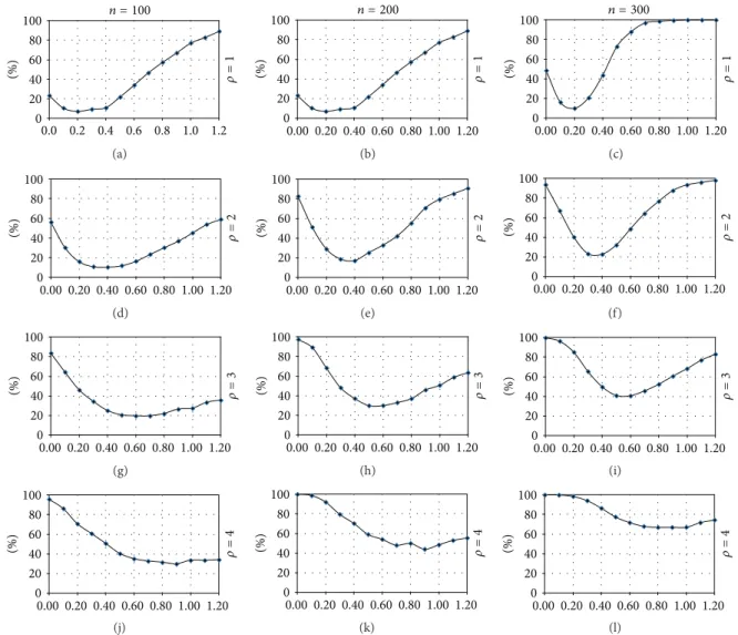
Figure 5: Power of the test against a mixture of clustered and repulsive point processes.𝑛 is the number of simulated points, 𝜌 a parameter of aggregation. Values are the ratio of simulated point patterns rejected by the test as a function of𝛽, a parameter indicating repulsion strength. See the text for complete explanations.
order to integrate all the information, steps between𝑟 values should be coherent with the processes to detect. 15 steps of 10 meters appear to be a correct way to test the structure of
Tachigali. 5-meter steps are too small considering the density
of the pattern (seeFigure 1), and 20-meter steps are too large for the process we consider.
4.4. Application of the Test: A User’s Guide. We provide a
test for a point pattern observed in a rectangular window against CSR. The code to run it with R is available as a supplementary material available online athttp://dx.doi.org/
10.1155/2013/753475. The function Ktest accepts a point
pat-tern object as defined in the spatstat package [31] and a vector of distancesr. It returns a 𝑃 value (the risk of error if CSR is rejected).
Distances should be chosen up to the range of possible interactions, with equal intervals small enough to describe correctly the pattern, but too many steps if points are few.
The maximum distance ̂𝐾(𝑟) is computed must be less than or
equal to half the width of the rectangle. This is a classical geo-metrical limitation, already faced by local edge-effect correc-tions [4] and [32, corrected up to half the length]. Rectangu-lar windows only are supported.
The test does not give information on what values ofr
are responsible for its significance. Practically, in order not to lose usual references, a graphical representation of𝐾 or,
better, its transformed function𝐿, should be provided with
local confidence intervals. If the number of points is great, the number of Monte-Carlo simulations can be reduced since these intervals are not used for the test.
5. Conclusion
Characterizing the spatial structure of a dataset representing the location of plants in an experimental plot is a common task for ecologists [33]. We provide a rigorous statistical test
to reject the null hypothesis that 𝐾 values of an observed
ISRN Ecology 7 of a homogenous Poisson point process. This test replaces
advantageously the classical Monte-Carlo one. It will rather complete it in practical applications since Monte-Carlo simu-lations provide useful local information on the point process. The test is ready to use with the provided R code to be found in the electronic appendices.
Future work includes both supporting more complex shapes, probably triangle assemblies following P´elissier and Goreaud [34], and other point processes as null hypotheses. Although it is still limited to the simplest applications, we believe this test is an important step towards more rigorous spatial statistics, based on analytical results rather than simulations.
Appendices
A. Variance and Covariance
We consider a point pattern in a rectangular window as
described in Section 2.2. 𝑟 and 𝑟 are two distances the
function is estimated at;𝑟is larger than𝑟. 𝐼(𝑁 > 1) is an indicator function equal to 1 when𝑁 > 1, 0 else. E(𝑋) is the
expectation of the random variable𝑋.
̂
𝐾(𝑟) is the estimator of Ripley’s 𝐾 function at distance 𝑟. The formulas of variance of ̂𝐾(𝑟) and covariance of ̂𝐾(𝑟) and ̂
𝐾(𝑟) are explicated here. A.1. Variance. One has
Var(̂𝐾 (𝑟)) = 2𝑙21𝑙22E (𝐼 (𝑁 > 1) 𝑁 (𝑁 − 1)) (𝑒𝑟,𝑙1,𝑙2− 𝑒2𝑟,𝑙1,𝑙2) + 4𝑙2 1𝑙22E ([𝐼 (𝑁 > 1)] (𝑁 − 2)𝑁 (𝑁 − 1) ) 𝑉 (𝑟, 𝑙1, 𝑙2) + 𝑙12𝑙22𝑒−𝜌𝑙1𝑙2(1 + 𝜌𝑙1𝑙2) × (1−𝑒−𝜌𝑙1𝑙2− 𝜌𝑙1𝑙2𝑒−𝜌𝑙1𝑙2) 𝑒2𝑟,𝑙1,𝑙2, (A.1) where 𝑒𝑟,𝑙1,𝑙2 = 𝜋𝑟2 𝑙1𝑙2 − 4𝑟3(𝑙1+𝑙2) 3𝑙1𝑙2 + 𝑟4 2𝑙2 1𝑙22, (A.2) 𝑉 (𝑟, 𝑛1, 𝑛2) = 𝑟5(𝑙1+𝑙2) 𝑙3 1𝑙32 ( 8 3𝜋 − 256 45 ) +𝑙𝑟36 1𝑙32( 11 48𝜋 − 8 9 − 16(𝑙1+𝑙2)2 𝑙1𝑙2 ) +4𝑟7(𝑙1+𝑙2) 3𝑙4 1𝑙24 − 𝑟8 4𝑙4 1𝑙42 , (A.3)
𝑒𝑟,𝑙1,𝑙2is the expectation of𝐾(𝑟) divided by the window’s area.
The main term is 𝜋𝑟2 divided by 𝑙1𝑙2 and the other terms
correspond to the bias due to edge effects.
𝜌 in (A.1) is unknown, so it is estimated by𝑁/(𝑙1𝑙2).
A.2. Covariance. One has
cov(̂𝐾 (𝑟) , ̂𝐾 (𝑟)) = 2𝑙2 1𝑙22E (𝑁 (𝑁 − 1)𝐼 (𝑁 > 1)) (𝑒𝑟,𝑙1,𝑙2− 𝑒𝑟,𝑙1,𝑙2𝑒𝑟,𝑙1,𝑙2) + 4𝑙12𝑙22E ([𝐼 (𝑁 > 1)] (𝑁 − 2) 𝑁 (𝑁 − 1) ) 𝐶 (𝑟, 𝑟, 𝑙1, 𝑙2) + 𝑙12𝑙22𝑒−𝜌𝑙1𝑙2(1 + 𝜌𝑙 1𝑙2) × (1−𝑒−𝜌𝑙1𝑙2− 𝜌𝑙 1𝑙2𝑒−𝜌𝑙1𝑙2) 𝑒𝑟,𝑙1,𝑙2𝑒𝑟,𝑙1,𝑙2, (A.4) where 𝐶 (𝑟, 𝑟, 𝑙1, 𝑙2) = (𝑙1− 2𝑟) (𝑙2− 2𝑟)𝑟 2𝑟2 𝑙3 1𝑙23 𝑏𝑟,𝑙1,𝑙2𝑏𝑟 ,𝑙 1,𝑙2 + 2 (𝑙1+ 𝑙2− 4𝑟)𝑟2𝑟3 𝑙3 1𝑙32 𝑏𝑟,𝑙1,𝑙2 × ∫1 𝑟/𝑟(𝑏𝑟,𝑙1,𝑙2− 𝑔 (𝑥 1)) 𝑑𝑥1 + 2 (𝑙1+ 𝑙2− 4𝑟)𝑟3𝑟2 𝑙3 1𝑙32 𝑏𝑟,𝑙1,𝑙2 × ∫1 0 (𝑏𝑟,𝑙1,𝑙2− 𝑔 ( 𝑟𝑥1 𝑟 )) (𝑏𝑟,𝑙1,𝑙2 −𝑔 (𝑥1)) 𝑑𝑥1 + 4𝑟2𝑟4 𝑙3 1𝑙32 ∫1 0 ∫ 1 0 [ℎ𝐴1( 𝑟𝑥 𝑟 , 𝑟) + ℎ𝐴2( 𝑟𝑥 𝑟 , 𝑟) +ℎ𝐴3(𝑟𝑥 𝑟 , 𝑟) + ℎ𝐴4( 𝑟𝑥 𝑟 , 𝑟)] × (ℎ𝐴3(𝑥, 𝑟) + ℎ𝐴4(𝑥, 𝑟)) 𝑑𝑥1𝑑𝑥2, (A.5) 𝑏𝑟,𝑙1,𝑙2 = 𝜋 − 𝑙1𝑙2 𝑟2 𝑒𝑟,𝑙1,𝑙2= − 4𝑟 (𝑙1+𝑙2) 3𝑙1𝑙2 + 𝑟2 2𝑙1𝑙2, (A.6) 𝑔 (𝑥) = 𝐼 (0 < 𝑥 < 1) (arccos 𝑥 + 𝑥√1 − 𝑥2) , (A.7) ℎ𝐴1(𝑥, 𝑟) = 𝑏𝑟,𝑙1,𝑙2𝐼 (𝑥1≥ 1) 𝐼 (𝑥2≥ 1) , ℎ𝐴2(𝑥, 𝑟) = (𝑏𝑟,𝑙1,𝑙2− 𝑔 (𝑥2)) 𝐼 (𝑥1≥ 1) 𝐼 (𝑥2< 1) + (𝑏𝑟,𝑙1,𝑙2− 𝑔 (𝑥1)) 𝐼 (𝑥2≥ 1) 𝐼 (𝑥1< 1) ,
ℎ𝐴3(𝑥, 𝑟) = (𝑏𝑟,𝑙1,𝑙2− 𝑔 (𝑥1) − 𝑔 (𝑥2))
× 𝐼 (𝑥1< 1) 𝐼 (𝑥2< 1) 𝐼 (𝑥21+ 𝑥22≥ 1) , ℎ𝐴4(𝑥, 𝑟) = (𝑏𝑟,𝑙1,𝑙2−𝜋4 + 𝑥1𝑥2−𝑔 (𝑥1) + 𝑔 (𝑥2 2))
× 𝐼 (𝑥21+ 𝑥22≤ 1) .
(A.8) E(𝐼(𝑁 > 1)/𝑁(𝑁 − 1)) and E([𝐼(𝑁 > 1)](𝑁 − 2)/𝑁(𝑁 − 1))
are estimated by1/𝑁(𝑁 − 1) and (𝑁 − 2)/𝑁(𝑁 − 1) as 𝑁
follows a Poisson law [11].
B. Power Test
Grabarnik and Chiu [30] proposed a new statistic (𝑄2) to test data against complete spatial randomness.𝑄2is of little use in practical situations because it suffers edge effects with no correction for them. We are interested here in the power test proposed by the authors. From a mathematical point of view, mixtures of a clumped and a repulsive point process are an interesting challenge for a test built to reject Poisson processes
whose𝐾 values are intermediate. From an ecological point of
view, these patterns make sense if we think of the processes responsible for, say, tree locations; aggregation is expected in regeneration processes and repulsion in competition pro-cesses. For example, Aldrich et al. [35] study the relative importance of the two processes along 60 years of the life of a forest.
We drew the same simulations as a power test. 𝑛 (100,
200, or 300) is the number of points of the simulated point
pattern in a window of area𝑛/200. Half of them are drawn
in a Mat´ern [36] process whose centers are drawn uniformly in the window (centers are not included in the point pattern) and offsprings are drawn less than 0.06 apart from centers. The number of offsprings around each center is drawn in a Poisson law of expectation𝜌 (1, 2, 3, or 4). Centers are added
until the number of offsprings reaches𝑛/2. The other half
of points is drawn in a Strauss [37] process with interaction
radius 0.06 and interaction parameter𝛽. Actually, Grabarnik
and Chiu used a Gibbs process with a fixed number of points [7] where𝛽 is the pair potential function (from 0 for no interaction to 1.2 for strong repulsion). The interaction parameter in usual presentations of the Strauss process (see [38, page 85]) is𝑒−𝛽. For each parameter set (𝑛, 𝜌, 𝛽), 10,000 point sets are drawn and tested against CSR. Results are
summarized inFigure 5.
Increasing the number of points (going right in the figure) improves the power of the test. Clustering increases with 𝜌 (going down the figure) while repulsion increases with 𝛽 (going right along curves). The result is the ratio of rejected simulations at a 5% risk level. It should be above 95% if the test was perfect but the point pattern is designed to be difficult to test, especially when parameters are all small (few clusters,
no repulsion; the process is close to Poisson) or intermediate (clustering of some points compensates repulsion of others). Grabarnik and Chiu rejected CSR when the maximum
departure of𝐾 from 𝜋𝑟2excessed that of 95% of a simulated
binomial process of𝑛 points. A comparison betweenFigure 5
and theirFigure 2shows that powers are similar, even though their test is too optimistic according to Loosmore and Ford [8].
In summary, we can see here that the tendencies observed
for the 𝐾 function’s power with Monte-Carlo simulations
remain valid. 𝐾 is not very efficient to disentangle mixed
clustered and repulsive point processes with both high𝜌 and
high𝛽 (Grabarnik and Chiu showed that Diggle’s 𝐺 is better
for that purpose) but rather powerful to detect clustering.
Acknowledgment
This work has benefited from an “Investissement d’Avenir” Grant managed by Agence Nationale de la Recherche (CEBA, ref. ANR-10-LABX-0025).
References
[1] B. D. Ripley, “The second-order analysis of stationary point processes,” Journal of Applied Probability, vol. 13, no. 2, pp. 255– 266, 1976.
[2] B. D. Ripley, “Modelling spatial patterns,” Journal of the Royal
Statistical Society B, vol. 39, no. 2, pp. 172–212, 1977.
[3] B. D. Ripley, Spatial Statistics, John Wiley & Sons, New York, NY, USA, 1981.
[4] P. J. Diggle, Statistical Analysis of Spatial Point Patterns, Aca-demic Press, London, UK, 1983.
[5] D. Stoyan, W. S. Kendall, and J. Mecke, Stochastic Geometry and
Its Applications, John Wiley & Sons, New York, NY, USA, 1987.
[6] N. A. Cressie, Statistics for Spatial Data, John Wiley & Sons, New York, NY, USA, 1993.
[7] J. Illian, A. Penttinen, H. Stoyan, and D. Stoyan, Statistical
Anal-ysis and Modelling of Spatial Point Patterns, Wiley-Interscience,
Chichester, UK, 2008.
[8] N. B. Loosmore and E. D. Ford, “Statistical inference using the G or K point pattern spatial statistics,” Ecology, vol. 87, no. 8, pp. 1925–1931, 2006.
[9] G. Duranton and H. G. Overman, “Testing for localization using micro-geographic data,” Review of Economic Studies, vol. 72, no. 4, pp. 1077–1106, 2005.
[10] E. Marcon and F. Puech, “Measures of the geographic con-centration of industries: improving distance-based methods,”
Journal of Economic Geography, vol. 10, no. 5, pp. 745–762, 2010.
[11] G. Lang and E. Marcon, “Testing randomness of spatial point patterns with the Ripley statistic,” ESAIM: Probability and
Statistics, 2013.
[12] R Development Core Team, R: A Language and Environment for
Statistical Computing, R Foundation for Statistical Computing,
Vienna, Austria, 2013.
[13] S. Gourlet-Fleury, J. M. Guehl, and O. Laroussinie, Eds., Ecology
& Management of a Neotropical Rainforest. Lessons Drawn from Paracou, a Long-Term Experimental Research Site in French Guiana, Elsevier, Paris, France, 2004.
[14] F. Goreaud, B. Courbaud, and F. Collinet, “Spatial struc-ture analysis applied to modelling of forest dynamics: a few
ISRN Ecology 9
examples,” in Proceedings of the IUFRO Workshop: Empirical
and Process-Based Models for Forest Tree and Stand Growth Simulation, A. Amaro and M. Tom´e, Eds., pp. 155–172, Novas
Tecnologias, Oeiras, Portugal, 1997.
[15] F. Collinet, Essai de regroupement des principales esp`eces
struc-turantes d’une forˆet dense humide d’apr`es leur r´epartition spatiale (forˆet de Paracou, Guyane) [Ph.D. thesis], Universit´e Claude
Bernard-Lyon I, Lyon, France, 1997.
[16] G. Jaouen, M. Fournier, and T. Almeras, “Thigmomorphogen-esis versus light in biomechanical growth strategies of saplings of two tropical rain forest tree species,” Annals of Forest Science, vol. 67, no. 2, p. 211, 2010.
[17] S. Coste, J. C. Roggy, L. Garraud, P. Heuret, E. Nicolini, and E. Dreyer, “Does ontogeny modulate irradiance-elicited plasticity of leaf traits in saplings of rain-forest tree species? A test with Dicorynia guianensis and Tachigali melinonii (Fabaceae, Caesalpinioideae),” Annals of Forest Science, vol. 66, no. 7, p. 709, 2009.
[18] O. Flores, S. Gourlet-Fleury, and N. Picard, “Local disturbance, forest structure and dispersal effects on sapling distribution of light-demanding and shade-tolerant species in a French Guianian forest,” Acta Oecologica, vol. 29, no. 2, pp. 141–154, 2006.
[19] J. E. Besag, “Comments on Ripley’s paper,” Journal of the Royal
Statistical Society B, vol. 39, no. 2, pp. 193–195, 1977.
[20] A. R. Clapham, “Over-dispersion in grassland communities and the use of statistical methods in plant ecology,” Journal of
Ecology, vol. 24, no. 1, pp. 232–251, 1936.
[21] P. G. Hoel, “On indices of dispersion,” The Annals of
Mathemat-ical Statistics, vol. 14, no. 2, pp. 155–162, 1943.
[22] P. J. Diggle, “On parameter estimation and goodness-of-fit testing for spatial point patterns,” Biometrics, vol. 35, no. 1, pp. 87–101, 1979.
[23] M. N. M. van Lieshout and A. J. Baddeley, “A nonparametric measure of spatial interaction in point patterns,” Statistica
Neerlandica, vol. 50, no. 3, pp. 344–361, 1996.
[24] J. Gignoux, C. Duby, and S. Barot, “Comparing the per-formances of Diggle’s tests of spatial randomness for small samples with and without edge-effect correction: application to ecological data,” Biometrics, vol. 55, no. 1, pp. 156–164, 1999. [25] B. D. Ripley, “Tests of ‘randomness’ for spatial point patterns,”
Journal of the Royal Statistical Society B, vol. 41, no. 3, pp. 368–
374, 1979.
[26] C. Koen, “Approximate confidence bounds for Ripley’s statistic for random points in a square,” Biometrical Journal, vol. 33, pp. 173–177, 1991.
[27] S. N. Chiu, “Correction to Koen’s critical values in testing spatial randomness,” Journal of Statistical Computation and Simulation, vol. 77, no. 11-12, pp. 1001–1004, 2007.
[28] E. Marcon and F. Puech, “Evaluating the geographic concen-tration of industries using distance-based methods,” Journal of
Economic Geography, vol. 3, no. 4, pp. 409–428, 2003.
[29] L. Heinrich, “Goodness-of-fit tests for the second moment function of a stationary multidimensional poisson process,”
Statistics, vol. 22, no. 2, pp. 245–268, 1991.
[30] P. Grabarnik and S. N. Chiu, “Goodness-of-fit test for complete spatial randomness against mixtures of regular and clustered spatial point processes,” Biometrika, vol. 89, no. 2, pp. 411–421, 2002.
[31] A. Baddeley and R. Turner, “Spatstat: an R package for analyzing spatial point patterns,” Journal of Statistical Software, vol. 12, no. 6, pp. 1–42, 2005.
[32] F. Goreaud and R. P´elissier, “On explicit formulas of edge effect correction for Ripley’s K-function,” Journal of Vegetation
Science, vol. 10, no. 3, pp. 433–438, 1999.
[33] R. Law, J. Illian, D. F. R. P. Burslem, G. Gratzer, C. V. S. Gunatilleke, and I. A. U. N. Gunatilleke, “Ecoogical information from satial patterns of plants: insights from point process theory,” Journal of Ecology, vol. 97, no. 4, pp. 616–628, 2009. [34] R. P´elissier and F. Goreaud, “A practical approach to the study
of spatial structure in simple cases of heterogeneous vegetation,”
Journal of Vegetation Science, vol. 12, no. 1, pp. 99–108, 2001.
[35] P. R. Aldrich, G. R. Parker, J. S. Ward, and C. H. Michler, “Spatial dispersion of trees in an old-growth temperate hardwood forest over 60 years of succession,” Forest Ecology and Management, vol. 180, no. 1–3, pp. 475–491, 2003.
[36] B. Mat´ern, “Spatial variation,” Meddelanden fr˚an Statens
Skogs-forskningsinstitut, vol. 49, no. 5, pp. 1–144, 1960.
[37] D. J. Strauss, “A model for clustering,” Biometrika, vol. 62, no. 2, pp. 467–475, 1975.
[38] J. Møller and R. P. Waagepetersen, Statistical Inference and
Simulation for Spatial Point Processes, vol. 100, Chapman and
Submit your manuscripts at
http://www.hindawi.com
Forestry Research
International Journal ofHindawi Publishing Corporation
http://www.hindawi.com Volume 2014 Public Health
Hindawi Publishing Corporation
http://www.hindawi.com Volume 2014
Hindawi Publishing Corporation
http://www.hindawi.com Volume 2014
Ecosystems
Journal ofHindawi Publishing Corporation
http://www.hindawi.com Volume 2014
Meteorology
Advances inEcology
Hindawi Publishing Corporation
http://www.hindawi.com Volume 2014
Marine Biology
Journal ofHindawi Publishing Corporation
http://www.hindawi.com Volume 2014
Hindawi Publishing Corporation http://www.hindawi.com
Applied &
Environmental
Soil Science
Volume 2014 Advances inHindawi Publishing Corporation
http://www.hindawi.com Volume 2014
Environmental Chemistry Atmospheric Sciences
International Journal of Hindawi Publishing Corporation
http://www.hindawi.com Volume 2014 Hindawi Publishing Corporation
http://www.hindawi.com Volume 2014
Hindawi Publishing Corporation
http://www.hindawi.com Volume 2014
International Journal of
Geophysics
Hindawi Publishing Corporationhttp://www.hindawi.com Volume 2014 Geological ResearchJournal of
Earthquakes
Journal ofHindawi Publishing Corporation
http://www.hindawi.com Volume 2014
Biodiversity
International Journal ofHindawi Publishing Corporation
http://www.hindawi.com Volume 2014
Scientifica
Hindawi Publishing Corporationhttp://www.hindawi.com Volume 2014
Oceanography
International Journal ofHindawi Publishing Corporation
http://www.hindawi.com Volume 2014
The Scientific
World Journal
Hindawi Publishing Corporation
http://www.hindawi.com Volume 2014
Journal of Computational Environmental Sciences Hindawi Publishing Corporation
http://www.hindawi.com Volume 2014
Hindawi Publishing Corporation
http://www.hindawi.com Volume 2014