HAL Id: hal-01130731
https://hal.archives-ouvertes.fr/hal-01130731
Submitted on 12 Mar 2015
HAL is a multi-disciplinary open access
archive for the deposit and dissemination of
sci-entific research documents, whether they are
pub-lished or not. The documents may come from
teaching and research institutions in France or
abroad, or from public or private research centers.
L’archive ouverte pluridisciplinaire HAL, est
destinée au dépôt et à la diffusion de documents
scientifiques de niveau recherche, publiés ou non,
émanant des établissements d’enseignement et de
recherche français ou étrangers, des laboratoires
publics ou privés.
Estimating the granularity coefficient of a Potts-Markov
random field within an MCMC algorithm
Marcelo Alejandro Pereyra, Nicolas Dobigeon, Hadj Batatia, Jean-Yves
Tourneret
To cite this version:
Marcelo Alejandro Pereyra, Nicolas Dobigeon, Hadj Batatia, Jean-Yves Tourneret. Estimating the
granularity coefficient of a Potts-Markov random field within an MCMC algorithm. IEEE Transactions
on Image Processing, Institute of Electrical and Electronics Engineers, 2013, vol. 22 (n° 6), pp.
2385-2397. �10.1109/TIP.2013.2249076�. �hal-01130731�
O
pen
A
rchive
T
OULOUSE
A
rchive
O
uverte (
OATAO
)
OATAO is an open access repository that collects the work of Toulouse researchers and
makes it freely available over the web where possible.
This is an author-deposited version published in :
http://oatao.univ-toulouse.fr/
Eprints ID : 12372
To link to this article : DOI :10.1109/TIP.2013.2249076
URL :
http://dx.doi.org/10.1109/TIP.2013.2249076
To cite this version : Pereyra, Marcelo Alejandro and Dobigeon,
Nicolas and Batatia, Hadj and Tourneret, Jean-Yves
Estimating the
granularity coefficient of a Potts-Markov random field within an
MCMC algorithm
. (2013) IEEE Transactions on Image Processing,
vol. 22 (n° 6). pp. 2385-2397. ISSN 1057-7149
Any correspondance concerning this service should be sent to the repository
administrator:
[email protected]
Estimating the Granularity Coefficient
of a Potts-Markov Random Field within
a Markov Chain Monte Carlo Algorithm
Marcelo Pereyra, Nicolas Dobigeon, Hadj Batatia and Jean-Yves Tourneret
Abstract— This paper addresses the problem of estimating the
Potts parameter β jointly with the unknown parameters of a Bayesian model within a Markov chain Monte Carlo (MCMC) algorithm. Standard MCMC methods cannot be applied to this problem because performing inference on β requires computing the intractable normalizing constant of the Potts model. In the proposed MCMC method, the estimation of β is conducted using a likelihood-free Metropolis–Hastings algorithm. Experimental results obtained for synthetic data show that estimating β jointly with the other unknown parameters leads to estimation results that are as good as those obtained with the actual value of
β. On the other hand, choosing an incorrect value of β can
degrade estimation performance significantly. To illustrate the interest of this method, the proposed algorithm is successfully applied to real bidimensional SAR and tridimensional ultrasound images.
Index Terms— Bayesian estimation, Gibbs sampler, intractable
normalizing constants, mixture model, Potts-Markov field.
I. INTRODUCTION
M
ODELING spatial correlation in images is fundamental in many image processing applications. Markov ran-dom fields (MRFs) have been recognized as efficient tools for capturing these spatial correlations [1]–[8]. One particular MRF often used for Bayesian classification and segmentation is the Potts model, which generalizes the binary Ising model to arbitrary discrete vectors. The amount of spatial correla-tion introduced by this model is controlled by the so-calledgranularity coefficient β. In most applications, this important parameter is set heuristically by cross-validation.
This paper studies the problem of estimating the Potts coefficient β jointly with the other unknown parameters of a
Manuscript received April 12, 2012; revised October 25, 2012; accepted January 26, 2013. Date of publication February 26, 2013; date of current version April 17, 2013. This work was supported in part by the CAMM4D Project, Funded by the French FUI, the Midi-Pyrenees region, and the SuSTaIN Program - EPSRC under Grant EP/D063485/1 - the Department of Mathematics of the University of Bristol, and the Hypanema ANR under Project n_ANR-12-BS03-003. The associate editor coordinating the review of this manuscript and approving it for publication was Prof. Rafael Molina.
M. Pereyra is with the School of Mathematics, University of Bristol, University Walk BS8 1TW, U.K. (e-mail: [email protected]).
N. Dobigeon, H. Batatia, and J.-Y. Tourneret are with the Univer-sity of Toulouse, IRIT/INP-ENSEEIHT/T´eSA, Toulouse 31071, France (e-mail: [email protected]; [email protected]; jean-yves. [email protected]).
standard Bayesian image classification or segmentation prob-lem. More precisely, we consider Bayesian models defined by a conditional observation model with unknown parameters and a discrete hidden label vector z whose prior distribution is a Potts model with hyperparameter β (this Bayesian model is defined in Section II). From a methodological perspective, inference on β is challenging because the distribution f (z, β) depends on the normalizing constant of the Potts model (hereafter denoted as C(β)), which is generally intractable. This problem has received some attention in the recent image processing literature, as it would lead to fully unsupervised algorithms [9]–[13].
In this work we focus on the estimation of β within a Markov chain Monte Carlo (MCMC) algorithm that handles 2D or 3D data sets [14]–[18]. MCMC methods are powerful tools to handle Bayesian inference problems for which the minimum mean square error (MMSE) or the maximum a posteriori (MAP) estimators are difficult to derive analytically. MCMC methods generate samples that are asymptotically distributed according to the joint posterior of the unknown model parameters. These samples are then used to approximate the Bayesian estimators. However, standard MCMC methods cannot be applied directly to Bayesian problems based on the Potts model. Indeed, inference on β requires computing the normalizing constant of the Potts model C(β), which is generally intractable. Specific MCMC algorithms have been designed to estimate Markov field parameters in [19], [20] and more recently in [9], [10]. A variational Bayes algorithm based on an approximation of C(β) has also been recently proposed in [11]. Maximum likelihood estimation of β within expectation-maximization (EM) algorithms has been studied in [12], [13], [21]. The strategies used in these works for avoiding the computation of C(β) are summarized below.
A. Pseudo-Likelihood Estimators
One possibility to avoid evaluating C(β) is to eliminate it from the posterior distribution of interest. More precisely, one can define a prior distribution f (β) such that the nor-malizing constant cancels out from the posterior (i.e., f (β) ∝
C(β)1R+(β), where 1R+(·)is the indicator function on R+),
resulting in the so-called pseudo-likelihood estimators [22]. Although analytically convenient this approach can result in poor estimation unless β is small [23].
B. Approximation of C(β)
Another possibility is to approximate the normalizing constant C(β). Existing approximations can be classified into three categories: based on analytical developments, on sam-pling strategies or on a combination of both. A survey of the state-of-the-art approximation methods up to 2004 has been presented in [20]. The methods considered in [20] are the mean field, the tree-structured mean field and the Bethe energy (loopy Metropolis) approximations, as well as two sampling strategies based on Langevin MCMC algorithms. It is reported in [20] that mean field type approximations, which have been successfully used within EM [24], [25] and stochastic EM algorithms [26], generally perform poorly in MCMC algorithms. More recently, exact recursive expressions have been proposed to compute C(β) analytically [11]. However, to our knowledge, these recursive methods have only been successfully applied to small problems (i.e., for MRFs of size smaller than 40×40) with reduced spatial correlation β < 0.5. Another sampling-based approximation consists in estimat-ing C(β) by Monte Carlo integration [27, Ch. 3], at the expense of very substantial computation and possibly biased estimations (bias arises from the estimation error of C(β)). Better results can be obtained by using importance sampling or path sampling methods [28]. These methods have been applied to the estimation of β within an MCMC image processing algorithm in [19]. Although more precise than Monte Carlo integration, approximating C(β) by importance sampling or path sampling still requires substantial compu-tation and is generally unfeasible for large fields. This has motivated recent works that reduce computation by combining importance sampling with analytical approximations. More precisely, approximation methods that combine importance sampling with extrapolation schemes have been proposed for the Ising model (i.e., a 2-state Potts model) in [9] and for the 3-state Potts model in [10]. However, we have found that this extrapolation technique introduces significant bias [29].
C. Auxiliary Variables and Perfect Sampling
Recent works from computational statistics have estab-lished that it is possible to avoid computing C(β) within a Metropolis-Hastings (MH) MCMC algorithm [27] by intro-ducing carefully selected auxiliary random variables [30], [31]. In the work of Moller et al. [30], an auxiliary vector w distributed according to the same distribution as the label vector z (i.e., f (z|β)) is introduced. Metropolis-Hastings algorithms that do not require computing C(β) are then proposed to sample the joint distribution f (β, w|z), which admits the exact desired posterior density f (β|z) as marginal distribution [30]. Unfortunately this method suffers from a very low acceptance ratio that degrades severely as the dimen-sion of z increases, and is therefore unsuitable for image processing applications [29]. New auxiliary variable methods with considerably better acceptance ratios have been proposed in [31] by using several auxiliary vectors and sequential Monte Carlo samplers [32]. These methods could be interesting for estimating the Potts coefficient β. However they will not be considered in this work because they require substantial
computation and are generally too costly for image processing applications. An alternative auxiliary variable method based on a one-sample estimator of the ratio C(β)/C(β∗)has been
proposed in [33] and recently been improved by using several auxiliary vectors and sequential Monte Carlo samplers in [34] (the ratio C(β)/C(β∗)arises in the MCMC algorithm defined in Section III-C). More details on the application of [33] to the estimation of the Potts coefficient β are provided in a separate technical report [29].
D. Likelihood-Free Methods
Finally, it is possible to avoid computing the normalizing constant C(β) by using likelihood-free MCMC methods [35]. These methods circumvent explicit evaluation of intractable likelihoods within an MH algorithm by using a simulation-based approximation. More precisely, akin to the auxiliary variable method [30], an auxiliary vector w distributed accord-ing to the likelihood f (z|β) is introduced. MH algorithms that do not require evaluating f (z|β) (nor C(β)) can then be considered to generate samples that are asymptotically distrib-uted according to the exact posterior distribution f (β|z) [35]. Although generally unfeasible1, these exact methods have
given rise to the approximative Bayesian computation (ABC) framework [36], which studies likelihood-free methods to gen-erate samples from approximate posterior densities fǫ(β|z) ≈ f(β|z)at a reasonable computational cost. To our knowledge these promising techniques, that are increasingly regarded as “the most satisfactory approach to intractable likelihood
problems” [36], have not yet been applied to image processing problems.
The main contribution of this paper is to propose an ABC MCMC algorithm for the joint estimation of the label vector z, the granularity coefficient β and the other unknown parameters of a Bayesian segmentation problem based on a Potts model. The estimation of β is included within an MCMC algorithm through an ABC method particularly adapted to the Potts model and to large data sets. It is shown that the estimation of β can be easily integrated to existing MCMC algorithms where β was previously assumed to be known. Applications to large 2D and 3D images illustrate the performance of the proposed method.
The remainder of the paper is organized as follows: Bayesian models considered in this work are defined in Section II. Section III describes a generic hybrid Gibbs sampler which generates samples asymptotically distributed according to the approximate posterior distribution of these Bayesian models. The estimation of β using a likelihood-free algorithm is discussed in detail in Section IV. Experiments on synthetic and real data are presented in Sections V and VI respectively. Conclusions are finally reported in Section VI.
II. BAYESIANMODEL
Let rn ∈ R+ denote the nth observation, or voxel, in a
lexicographically vectorized image r = (r1, . . . , rN)T ∈ RN.
1In spite of being theoretically correct, exact likelihood-free algorithms
suffer from several major shortcomings that make them generally impractical (see Section IV for more details).
We assume that r is made up by multiple regions, charac-terized by their own statistics. More precisely, r is assumed to be associated with K stationary classes {C1, . . . , CK} such
that the observations in the kth class are fully described by the following conditional observation model
rn|zn= k ∼ f !rn|θk
"
(1) where f !rn|θk
"
denotes a generic observation model with parameter vector θkcharacterizing the class Ck. Finally, a label
vector z = (z1, . . . , zN)T is introduced to map observations r
to classes C1, . . . , CK (i.e., zn= k if and only if rn∈ Ck).
Several works have established that a Potts model can be used to exploit the fact that the probability P[zn = k] of a
given voxel is related to the probabilities of its neighbors. The amount of spatial correlation between adjacent image pixels introduced by the Potts model is controlled by the granularity coefficient β. Existing image classification and segmentation methods have mainly studied the estimation of the class parameter vector θ = (θT1, . . . , θTK)T and the label
vector z conditionally to a known value of β. However, setting β incorrectly can degrade the estimation of θ and
z significantly. Moreover, fixing the value of β a priori is difficult because different images can have different spatial organizations. This paper considers the problem of estimating the unknown parameter vectors θ and z jointly with β from the observation vector r. This problem is formulated in a Bayesian framework which requires to define the likelihood of the observation vector r and the priors for the unknown parameters θ , z and β.
A. Likelihood
Assuming that the observations rn are independent
condi-tionally to the label vector z, the likelihood function associated with the image r is
f(r|θ , z, β) = f (r|θ , z) = K # k=1 # {n|zn=k} f(rn|θk) (2)
where f (rn|θk) is the generic probability density function
associated with the observation model introduced in (1).
B. Parameter Priors
1) Labels: It is natural to consider that there are some cor-relations between the characteristics of a given voxel and those of its neighbors. Since the seminal work of Geman [1], MRFs have become very popular to introduce spatial correlation in images [2], [7], [8], [24], [37], and [38]. MRFs assume that the distribution of a pixel conditionally to all other pixels of the image equals the distribution of this pixel conditionally to its neighbors
f (zn|z−n) = f!zn|zV (n)" (3)
where V(n) is the index set of the neighbors of the nth voxel (the neighborhoods used in this paper for 2D and 3D images are depicted in Fig. 1), z−n denotes the vector z whose nth
element has been removed and zV (n) is the sub-vector of z
composed of the elements whose indexes belong to V(n).
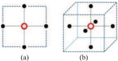
(a) (b)
Fig. 1. (a) Four-pixel and (b) six-voxel neighborhood structures. The pixel/voxels considered appear as a void red circle whereas its neighbors are depicted in full black and blue.
In the case of K classes, the random variables z1, z2, . . . , zN
take their values in the finite set {1, . . . , K }. The resulting MRF (with discrete values) is a Potts-Markov field, which generalizes the binary Ising model to arbitrary discrete vectors. In this study, 2D and 3D Potts-Markov fields will be considered as prior distributions for z. More precisely, 2D MRFs are considered for single-slice (2D) images whereas 3D MRFs are investigated for multiple-slice (3D) images. Note that Potts-Markov fields are particularly well suited for label-based segmentation as explained in [39]. By the Hammersley-Clifford theorem the corresponding prior for
zcan be expressed as follows
f(z|β) = 1 C(β)exp$8β(z) % (4) where 8β(z) = N & n=1 & n′∈V (n) βδ(zn− zn′) (5)
and where δ(·) is the Kronecker function, β is the granularity coefficient and C(β) is the partition function [37]
C(β) = &
z∈{1,...,K }n
exp$8β(z)% . (6)
As explained previously, the normalizing constant C(β) is generally intractable even for K = 2 because the number of summands in (6) grows exponentially with the size of z [40]. The hyperparameter β tunes the degree of homogeneity of each region in the image. A small value of β induces a noisy image with a large number of regions, contrary to a large value of β that leads to few and large homogeneous regions. Finally, it is interesting to note that despite not knowing C(β), drawing labels z = (z1, . . . , zN)T from the distribution (4)
can be easily achieved by using a Gibbs sampler [27].
2) Parameter Vector θ : Assuming a priori independence between the parameters θ1, . . . , θK, the joint prior for the
parameter vector θ is f (θ ) = K # k=1 f(θk) (7)
where f (θk)is the prior associated with the parameter vector
θkwhich mainly depends on the application considered. Two
examples of priors f (θ) will be investigated in Section V.
3) Granularity Coefficient β: As explained previously, fixing the value of β a priori can be difficult because different images usually have different spatial organizations. A small value of β will lead to a noisy classification and degrade the estimation of θ and z. Setting β to a too large value will also
degrade the estimation of θ and z by producing over-smoothed classification results. Following a Bayesian approach, this paper proposes to assign β an appropriate prior distribution and to estimate this coefficient jointly with (θ, z). In this work, the prior for β is a uniform distribution on (0, B)
f(β) = U(0,B)(β) (8)
where B represents the maximum possible value of β (the experiments in this work have been conducted using B = 10).
C. Posterior Distribution of(θ , z, β)
Assuming prior independence between θ and (z, β) and using Bayes theorem, the posterior distribution of (θ , z, β) can be expressed as follows
f(θ , z, β|r) ∝ f (r|θ, z) f (θ) f (z|β) f (β) (9) where ∝ means “proportional to” and where the likelihood
f(r|θ , z) has been defined in (2) and the prior distributions
f(θ), f (z|β) and f (β) in (7), (4) and (8) respectively. Unfortunately the posterior distribution (9) is generally too complex to derive the MMSE or MAP estimators of the unknown parameters θ , z and β. An interesting alternative consists in using an MCMC method that generates samples that are asymptotically distributed according to the target distribution (9) [27]. The generated samples are then used to approximate the Bayesian estimators. Despite their high computational cost, MCMC methods are increasingly used to solve difficult inference problems and have been applied successfully in several recent image processing applications (see [15], [16], [41]–[45] for examples in image filtering, dictionary learning, image reconstruction, fusion and segmen-tation). Many of these recent MCMC methods have been proposed for Bayesian models that include a Potts MRF [14], [15], [17], [18], [43]. However, these methods only studied the estimation of θ and z conditionally to a known granularity coefficient β. The main contribution of this paper is to study Bayesian algorithms for the joint estimation of θ , z and β. The next section studies a hybrid Gibbs sampler that generates samples that are asymptotically distributed according to the posterior (9). The samples are then used to estimate the granularity coefficient β, the image labels z and the model parameter vector θ . The resulting sampler can be easily adapted to existing MCMC algorithms where β was previously assumed known, and can be applied to large 2D and 3D images. It is worth mentioning that MCMC methods are not the only strategies that can be used for estimating θ , z, β. Indeed, for many problems one can use the EM algorithm, which has received much attention for mixture problems [46]. In these cases the estimation of β can be addressed using mean field approximations [24]–[26], [47].
III. HYBRIDGIBBSSAMPLER
This section studies a hybrid Metropolis-within-Gibbs sam-pler that generates samples that are asymptotically distributed according to (9). The conventional Gibbs sampler successively draws samples according to the full conditional distributions
Algorithm 1Proposed Hybrid Gibbs Sampler
associated with the distribution of interest (here the poste-rior (9)). When a conditional distribution cannot be easily sampled, one can resort to an MH move, which generates samples according to an appropriate proposal and accept or reject these generated samples with a given probability. The resulting sampler is referred to as a Metropolis-within-Gibbs sampler (see [27] for more details about MCMC methods). The sampler investigated in this section is based on the condi-tional distributions P[z|θ, β, r], f (θ |z, β, r) and f (β|θ , z, r) that are provided in the next paragraphs (see also Algorithm 1 below).
A. Conditional ProbabilityP[z|θ , β, r]
For each voxel n ∈ {1, 2, . . . , N}, the class label zn is a
discrete random variable whose conditional distribution is fully characterized by the probabilities
P$zn= k|z−n, θk, β, r% ∝ f (rn|θk, zn= k)
P$zn= k|zV (n), β
%
(10) where k = 1, . . . , K , and where it is recalled that V(n) is the index set of the neighbors of the nth voxel and K is the number of classes. These probabilities can be expressed as
P$zn= k|zV (n), θk, β, r% ∝ πn,k (11) with πn,k, exp & n′∈V (n) βδ(k − zn′) f(rn|θk, zn= k).
Once all the quantities πn,k, k = 1, . . . , K , have been
computed, they are normalized to obtain the probabilities ˜ πn,k, P $zn= k|zV (n), θk, β, r% as follows ˜ πn,k= πn,k +K k=1πn,k . (12)
Note that the probabilities of the label vector z in (12) define an MRF. Sampling from this conditional distribution can be achieved by using a Gibbs sampler [27] that draws discrete values in the finite set {1, . . . , K } with probabilities (12). More precisely, in this work z has been sampled using a 2-color parallel chromatic Gibbs sampler that loops over n ∈ {1, 2, . . . , N} following the checkerboard sequence [48].
B. Conditional Probability Density Function f(θ |z, β, r) The density f (θ|z, β, r) can be expressed as follows
f(θ |z, β, r) = f (θ |z, r) ∝ f (r|θ , z) f (θ) (13) where f (r|θ , z) and f (θ) have been defined in (2) and (7). Generating samples distributed according to (13) is strongly problem dependent. Some possibilities will be discussed in Sections V and VI. Generally, θ = (θT1, . . . , θTK)T can be
sampled coordinate-by-coordinate using the following Gibbs moves θk∼ f (θk|r, z) ∝ # {n|zn=k} f(rn|θk) f (θk), k =1, . . . , K . (14) In cases where sampling the conditional distribution (14) is too difficult, an MH move can be used resulting in a Metropolis-within-Gibbs sampler [27] (details about the generation of samples θk for the problems studied in Sections V and VI
are provided in a separate technical report [29]).
C. Conditional Probability Density Function f(β|θ, z, r) From Bayes rule, the conditional density f (β|θ, z, r) can be expressed as follows
f(β|θ, z, r) = f (β|z) ∝ f (z|β) f (β) (15) where f (z|β) and f (β) have been defined in (4) and (8) respectively. The generation of samples according to
f(β|θ, z, r)is not straightforward because f (z|β) is defined up to the unknown multiplicative constant 1/C(β) that depends on β. One could think of sampling β by using an MH move, which requires computing the acceptance ratio
ratio = min {1, ξ } (16) with ξ = f(z|β ∗) f(z|β(t −1)) f(β∗) f(β(t −1)) q(β(t −1)|β∗) q(β∗|β(t −1)) (17)
where β∗ ∼ q(β∗|β(t −1)) denotes an appropriate proposal distribution. Replacing (4) into (17), ξ can be expressed as
ξ = C(β (t −1)) C(β∗) exp$8β∗(z)% exp$8β(t−1)(z)% f(β∗) f(β(t −1)) q(β(t −1)|β∗) q(β∗|β(t −1)) (18) where β∗ denotes the proposed value of β at iteration t and β(t −1) is the previous state of the chain. Unfortunately the ratio (18) is generally intractable because of the term C(βC(β(t−1)∗)).
The next section presents a likelihood-free MH algorithm that samples β without requiring to evaluate f (z|β) and C(β).
IV. SAMPLING THEGRANULARITYCOEFFICIENT A. Likelihood-Free Metropolis–Hastings
It has been shown in [35] that it is possible to define a valid MH algorithm for posterior distributions with intractable likelihoods by introducing a carefully selected auxiliary vari-able and a tractvari-able sufficient statistic on the target density. More precisely, consider an auxiliary vector w defined in the
Algorithm 2Exact Likelihood-Free MH Step [35]
discrete state space {1, . . . , K }N of z generated according to the likelihood f (z|β), i.e.,
w ∼ f(w|β), 1
C(β)exp$8β(w)% . (19) Also, let η(z) be a tractable sufficient statistic of z, i.e.,
f(β|z) = f [β|η(z)]. Then, it is possible to generate samples that are asymptotically distributed according to the exact conditional density f (β|θ, z, r) = f (β|z) by introducing an additional rejection step based on η(z) into a standard MH move. Details about this sampler are provided in Algorithm 2. Note that the MH acceptance ratio in algorithm 2 is the product of the prior ratio f (β∗)/ f (β(t −1)) and the proposal ratio q(β(t −1)|β∗)/q(β∗|β(t −1)). The generally intractable
likelihood ratio f (z|β∗)/ f (z|β(t −1))has been replaced by the simulation and rejection steps involving the discrete auxiliary vector w. The resulting MH move still accepts candidate val-ues β∗with the correct probability (16) and has the advantage of not requiring to evaluate the ratio f (z|β∗)/ f (z|β(t −1)) explicitly [35].
Unfortunately exact likelihood-free MH algorithms have several shortcomings [36]. For instance, their acceptance ratio is generally very low because candidates β∗are only accepted if they lead to an auxiliary vector w that verifies η(z(t )) = η(w). In addition, most Bayesian models do not have known sufficient statistics. These limitations have been addressed in the ABC framework by introducing an approximate likelihood-free MH algorithm (henceforth denoted as ABC-MH) [35]. Precisely, the ABC-MH algorithm does not require the use of a sufficient statistic and is defined by a less restrictive criterion of the form ρ$η(z(t )), η(w)% < ǫ, where η is a statistic whose
choice will be discussed in Section IV-B, ρ is an arbitrary distance measure and ǫ is a tolerance parameter (note that this criterion can be applied to both discrete and continuous intractable distributions, contrary to algorithm 2 that can only be applied to discrete distributions). The resulting algorithm generates samples that are asymptotically distributed according to an approximate posterior density [35]
fǫ(β|z) ≈
&
w
whose accuracy depends on the choice of η(z) and ǫ (if η(z) is a sufficient statistic and ǫ = 0, then (20) corresponds to the exact posterior density).
In addition, note that in the exact likelihood-free MH algorithm, the auxiliary vector w has to be generated using perfect sampling [49], [50]. This constitutes a major limitation, since perfect or exact sampling techniques [49], [50] are too costly for image processing applications where the dimension of z and w can exceed one million of pixels. A convenient alternative is to replace perfect simulation by a few Gibbs moves with target density f (w|β∗) as proposed in [51]. The accuracy of this second approximation depends on the number of moves and on the initial state of the sampler. An infinite number of moves would clearly lead to perfect simulation regardless of the initialization. Inspired from [52], we propose to use z as initial state to produce a good approximation with a small number of moves. A simple explanation for this choice is that for candidates β∗close to the mode of f (β|z), the vector
zhas a high likelihood f (z|β). In other terms, using z as initial
state does not lead to perfect sampling but provides a good final approximation of f (β|z) around its mode. The accuracy of this approximation can be easily improved by increasing the number of moves at the cost of a larger computational complexity. However, several simulation results in [29], [34] have shown that the resulting ABC algorithm approximates
f(β|z)correctly even for a small number of moves.
B. Choice of η(z), ρ, and ǫ
As explained previously, ABC algorithms require defining an appropriate statistic η(z), a distance function ρ and a tolerance level ǫ. The choice of η(z) and ρ are fundamental to the success of the approximation, while the value of ǫ is generally less important [36]. Fortunately the Potts MRF, being a Gibbs random field, belongs to the exponential family and has the following one-dimensional sufficient statistic [36], [51]
η(z), N & n=1 & n′∈V (n) δ(zn− zn′) (21)
where it is recalled that V(n) is the index set of the neighbors of the nth voxel. Note that because (21) is a sufficient statistic, the approximate posterior fǫ(β|z)tends to the exact posterior
f(β|z)as ǫ → 0 [35].
The distance function ρ considered in this work is the one-dimensional Euclidean distance
ρ[η(z), η(w)] = |η(z) − η(w)| (22) which is a standard choice in ABC methods [36]. Note from (21) and (22) that the distance ρ[·, ·] between η(z) and η(w)reduces to the difference in the number of active cliques in z and w. It is then natural to set the tolerance as a fraction of that number, i.e., ǫ = νη(z) (ν = 10−3 will be used in our experiments). Note that the choice of ν is crucial when the prior density f (β) is informative because increasing ν introduces estimation bias by allowing the posterior density to drift towards the prior [53]. However, in this work, the choice of ν is less critical because β has been assigned a flat prior.
Algorithm 3ABC Likelihood-Free MH Step [35]
C. Proposal Distribution q(β∗|β(t −1))
Finally, the proposal distribution q(β∗|β(t −1)) used to explore the set (0, B) is chosen as a truncated normal distribution centered on the previous value of the chain with variance sβ2 β∗∼ N(0,B) , β(t −1), sβ2 -. (23)
The variance sβ2is adjusted during the burn-in period to ensure an acceptance ratio close to 5%, as recommended in [29]. This proposal strategy is referred to as random walk MH algorithm [27, p. 287]. The choice of this proposal distribution has been motivated by the fact that for medium and large problems (i.e., Markov fields larger than 50 × 50 pixels) the distribution f (β|z) becomes very sharp and can be efficiently explored using a random walk (note that f (β|z) depends implicitly on the size of the problem through (5) and (6)).2
The resulting ABC MH method is summarized in Algorithm 3 below. Note that Algorithm 3 corresponds to step 5 in Algorithm 1.
D. Computational Complexity
A common drawback of MCMC methods is their computation complexity, which is significantly higher than that of deterministic inference algorithms. The introduction of Algorithm 3 to estimate β increases the complexity of Algorithm 1 by a factor of M + 1 with respect to the case where β is fixed (M is the number of Gibbs iterations used to generate the auxiliary variable w in line 3 of Algorithm 3). Precisely, for an N-pixel image, sampling (z, θ , β) requires generating N(M + 1) + dim θ + 1 ≈ N(M + 1) random variables per iterations, as opposed to N + dim θ ≈ N when β is fixed. In other terms, estimating β requires sampling the Potts field M + 1 times per iteration, once to update z, and M
2Alternatively, for smaller problems one could also consider a Beta
distribution on (0, B) as proposal for β∗, resulting in an independent MH algorithm [27, p. 276].
TABLE I ESTIMATION OFβ
True β Aux. var [30] Exch. [33] ES [10] ABC-MH (Algo. 3) β =0.2 0.20 ± 0.03 0.21 ± 0.03 0.21 ± 0.02 0.20 ± 0.03
β =0.6 0.61 ± 0.03 0.60 ± 0.03 0.45 ± 0.04 0.60 ± 0.02
β =1.0 1.01 ± 0.03 1.00 ± 0.02 0.77 ± 0.05 1.00 ± 0.02
β =1.4 1.37 ± 0.06 1.41 ± 0.04 1.38 ± 0.02 1.41 ± 0.04
times to generate the auxiliary variable w. In this work w has been sampled using M = 3 Gibbs moves, as recommended in [52]. Note that the complexity of the proposed method also scales linearly with the the number of image pixels N.
Moreover, in this work the number of burn-in iterations required to reach stationarity has been determined by tracing the chains of θ and β (note that computing quantitative conver-gence indicators [54] would be extremely computationally and memory intensive because of the high complexity of Algo 3). Similarly, the total number of iterations (denoted as T in Algorithm 1) has been determined by checking that the MMSE estimates ˆθ and ˆβ do not change significantly when including additional iterations.
V. EXPERIMENTS
This section presents simulation results conducted on syn-thetic data to assess the importance of estimating the hyper-parameter β from data as opposed to fixing it a priori (i.e., the advantage of estimating the posterior p(θ, z, β|r) instead of fixing β). Simulations have been performed as follows: label vectors distributed according to a Potts MRF have been generated using different granularity coefficients (in this section bidimensional fields of size 256 × 256 pixels have been considered). Each label vector has in turn been used to generate an observation vector following the observation model (1). Finally, samples distributed according to the poste-rior distribution of the unknown parameters (θ , z, β) have been estimated from each observation vector using Algorithm 1 coupled with Algorithm 3 (assuming the number of classes
K is known). The performance of the proposed algorithm has been assessed by comparing the Bayesian estimates with the true values of the parameters. In all experiments the parameter vector θ and the labels z have been initialized randomly. Conversely, we have used β(0) = 1.0 as initial condition for the granularity parameter. This choice has been motivated by the fact that initializing β at a too large value degrades the mixing properties of the sampler and leads to very long burn-in periods. Finally, note that the experiments reported hereafter have been computed on a workstation equipped with an Intel Core 2 Duo @2.1 GHz processor, 3MB L2 and 3GB of RAM memory. The main loop of the Gibbs sampler has been implemented on MATLAB R2010b. However, C-MEX functions have been used to simulate samples z and w.
This paper presents simulation results obtained using two different mixture models. Additional simulation results using other mixture models are available in a separate technical report [29]. Detailed comparisons with the state-of-the-art methods proposed in [10], [30], [33] are also reported in [29].
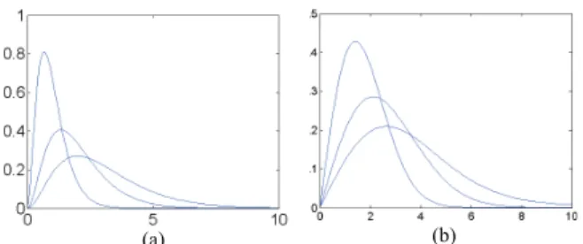
(a) (b)
Fig. 2. Probability density functions of the distributions mixed for the first set and the second set of experiments. (a) Gamma mixture. (b) α-Rayleigh mixture.
For completeness, a synthesis of one of these comparisons is presented in Table I, which shows the MMSE estimates of β corresponding to 3-state Potts MRFs simulated using different values of β. To ease interpretation, the best result for each simulation scenario has been highlighted in red. Details on how these estimates have been computed and other experiments comparing these methods can be found in [29]. All the simulations show that the proposed ABC-MH algorithm provides very good results.
A. Mixture of Gamma Distributions
The first experiment considers a mixture of gamma distrib-utions. This observation model is frequently used to describe the statistics of pixels in multilook SAR images and has been extensively applied for SAR image segmentation [55]. Accordingly, the conditional observation model (1) is defined by a gamma distribution with parameters L and mk [55]
rn|zn= k ∼ f (rn|θk) = . L mk /L rL−1 n Ŵ(L)exp . −Lrn mk / (24) where Ŵ(t) =0+∞ 0 ut −
1e−udu is the standard gamma
func-tion and L (the number of looks) is assumed to be known (L = 3 in this paper). The means mk (k = 1, . . . , K )
are assigned inverse gamma prior distributions as in [55]. The estimation of β, z and θ = m = (m1, . . . , mK)T is
then achieved by using Algorithm 1. The sampling strategies described in Sections III-A and IV can be used for the gener-ation of samples according to P[z|m, β, r] and f (β|m, z, r). More details about simulation according to f (m|z, β, r) are provided in the technical report [29].
The first results have been obtained for a 3-component gamma mixture with parameters m = (1; 2; 3). Fig. 2(a) shows the densities of the gamma distributions defining the mixture model. Note that there is a significant overlap between the densities making the inference problem very challenging. For each experiment the MAP estimates of the class labels z have been computed from a single Markov chain of T = 1 000 iterations whose first 400 iterations (burn-in period) have been removed. Precisely, these estimates have been computed individually for each voxel by calculating the mode of the discrete samples z(t )n (t = 400, . . . , T ). Table II shows the
percentage of MAP class labels correctly estimated. The first column corresponds to labels that were estimated jointly with β whereas the other columns result from fixing β to different a priori values. To ease interpretation, the best and second best
TABLE II
GAMMAMIXTURE: CLASSLABELESTIMATION(K = 3) Correct Classification With β Fixed Proposed Method β =0.6 β = 0.8 β = 1.0 β = 1.2 β = 1.4 ˆ β = 0.80 62.2% 61.6% 61.7% 58.8% 41.5% 40.1% ˆ β =1.00 77.9% 67.3% 73.4% 77.7% 75.9% 74.2% ˆ β =1.18 95.6% 76.6% 87.8% 94.9% 95.6% 95.5% TABLE III
GAMMAMIXTURE: PARAMETERESTIMATION
True MMSE True MMSE True MMSE β 0.80 0.80 ± 0.01 1.00 1.00 ± 0.01 1.20 1.18 ± 0.02 m1 1 0.99 ± 0.02 1 1.00 ± 0.02 1 0.99 ± 0.03
m2 2 1.99 ± 0.02 2 1.98 ± 0.02 2 1.98 ± 0.07
m3 3 2.98 ± 0.03 3 2.98 ± 0.04 3 3.01 ± 0.03
results for each simulation scenario in Table II are highlighted in red and blue. We observe that the proposed method performs as well as if β was perfectly known. On the other hand, setting β to an incorrect value may severely degrade estimation performance. The average computing times for this experiment were 151 seconds when estimating labels jointly with β and 69 seconds when β was fixed. Moreover, Table III shows the MMSE estimates of β and m corresponding to the three simulations of the first column of Table II (proposed method) as well as the standard deviations of the estimates (results are displayed as [mean ± standard deviation]). We observe that these values are in good agreement with the true values used to generate the observation vectors. Finally, for illustration purposes, Fig. 3 shows the MAP estimates of the class labels corresponding to the simulation scenario reported in the last row of Table II. More precisely, Fig. 3(a) depicts the class label map, which is a realization of a 3-class Potts MRF with β = 1.2. The corresponding synthetic image is presented in Fig. 3(b). Fig. 3(c) shows the class labels obtained with the proposed method and Fig. 3(d) those obtained when β is perfectly known. Lastly, Figs. 3(e)–(h) show the results obtained when β is fixed incorrectly to 0.6, 0.8, 1.0 and 1.4. We observe that the classification produced by the proposed method is very close to that obtained by fixing β to its true value, whereas fixing β incorrectly results in either noisy or excessively smooth results.
B. Mixture ofα-Rayleigh Distributions
The second set of experiments has been conducted using a mixture of α-Rayleigh distributions. This observation model has been recently proposed to describe ultrasound images of dermis [56] and has been successfully applied to the segmentation of skin lesions in 3D ultrasound images [18]. Accordingly, the conditional observation model (1) used in the experiments is defined by an α-Rayleigh distribution
rn|zn= k ∼ f (rn|θk) = pαR(rn|αk, γk) (25)
(a) (b)
(c) (d)
(e) (f)
(g) (h)
Fig. 3. Gamma mixture: estimated labels using the MAP estimators. (a) Ground truth. (b) Observations. (c) Proposed algorithm (estimated β). (d) True β = 1.2. (e)-(h) Fixed β = (0.6, 0.8, 1.0, 1.2, 1.4).
with
pαR(rn|αk, γk), rn
1 ∞
0
λexp$−(γkλ)αk% J0(rnλ) dλ
where αk and γk are the parameters associated with the kth
class and where J0 is the zeroth order Bessel function of
the first kind. Note that this distribution has been also used to model SAR images in [57], [58]. The prior distributions assigned to the parameters αk and γk (k = 1, . . . , K ) are
uni-form and inverse gamma distributions as in [18]. The estima-tion of β, z and θ = (αT, γT)T = (α
1, . . . , αK, γ1, . . . , γK)T
is performed by using Algorithm 1. The sampling strate-gies described in Sections III-A and IV can be used for the generation of samples according to P[z|α, γ , β, r] and
f(β|α, γ , z, r). More details about simulation according to
f(α|γ , z, β, r) and f (γ |α, z, β, r) are provided in the tech-nical report [29].
The following results have been obtained for a 3-component α-Rayleigh mixture with parameters α = (1.99; 1.99; 1.80) and γ = (1.0; 1.5; 2.0). Fig. 2(b) shows the densities of the components associated with this α-Rayleigh mixture. Again, note that there is significant overlap between the mixture components making the inference problem very challenging.
TABLE IV
α-RAYLEIGHMIXTURE: CLASSLABELESTIMATION(K = 3) Correct Classification With β Fixed Proposed Method β = 0.6 β = 0.8 β = 1.0 β = 1.2 β = 1.4 ˆ β =0.81 56.5% 52.3% 56.3% 44.8% 33.3% 33.4% ˆ β =1.01 75.5% 61.1% 68.1% 75.5% 54.1% 41.7% ˆ β = 1.18 95.0% 67.7% 83.1% 94.4% 94.8% 69.5%
For each experiment the MAP estimates of the class labels z have been computed from a single Markov chain of T = 2 000 iterations whose first 900 iterations (burn-in period) have been removed. Again, these estimates have been computed individually for each voxel by calculating the mode of the discrete samples z(t )n (t = 900, . . . , T ). Table IV shows the
percentage of MAP class labels correctly estimated. The first column corresponds to labels that were estimated jointly with β whereas the other columns result from fixing β to different a priori values. To ease interpretation, the best and second best results for each simulation scenario in Table IV are highlighted in red and blue. We observe that even if the mixture com-ponents are hard to estimate, the proposed method performs similarly to the case of a known coefficient β. Also, setting β incorrectly degrades estimation performance considerably. The average computing times for this experiment were 199 seconds when estimating labels jointly with β and 116 seconds when β was fixed. Moreover, Table V shows the MMSE estimates of β, α and γ corresponding to the three simulations of the first column of Table IV (proposed method). We observe that these values are in good agreement with the true values used to generate the observation vectors. To conclude, Fig. 4 shows the MAP estimates of the class labels corresponding to the simulation associated with the scenario reported in the last row of Table IV. More precisely, the actual class labels are displayed in Fig. 4(a), which shows a realization of a 3-class Potts MRF with β = 1.2. The corresponding observation vector is presented in Fig. 4(b). Fig. 4(c) and Fig. 4(d) show the class labels obtained with the proposed method and with the actual value of β. Lastly, Figs. 4(e)–(h) show the results obtained when β is fixed incorrectly to 0.6, 0.8, 1.0 and 1.4. We observe that the proposed method produces classification results that are very similar to those obtained when β is fixed to its true value. On the other hand, fixing β incorrectly generally leads to very poor results.
VI. APPLICATION TOREALDATA
After validating the proposed Gibbs sampler on synthetic data, this section presents two applications of the proposed algorithm to real data. Supplementary experiments using real data are provided in the technical report [29].
A. Pixel Classification of a 2D SAR Image
The proposed method has been applied to the unsupervised classification of a 2D multilook SAR image acquired over Toulouse, France, depicted in Fig. 5(a) (the same region observed by an airborne optical sensor is shown in Fig. 5(b)).
TABLE V
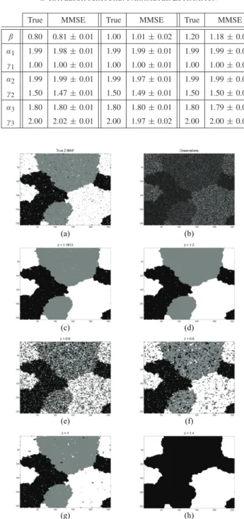
α-RAYLEIGHMIXTURE: PARAMETERESTIMATION
True MMSE True MMSE True MMSE β 0.80 0.81 ± 0.01 1.00 1.01 ± 0.02 1.20 1.18 ± 0.02 α1 1.99 1.98 ± 0.01 1.99 1.99 ± 0.01 1.99 1.99 ± 0.01 γ1 1.00 1.00 ± 0.01 1.00 1.00 ± 0.01 1.00 1.00 ± 0.01 α2 1.99 1.99 ± 0.01 1.99 1.97 ± 0.01 1.99 1.99 ± 0.01 γ2 1.50 1.47 ± 0.01 1.50 1.49 ± 0.01 1.50 1.50 ± 0.01 α3 1.80 1.80 ± 0.01 1.80 1.80 ± 0.01 1.80 1.79 ± 0.01 γ3 2.00 2.02 ± 0.01 2.00 1.97 ± 0.02 2.00 2.00 ± 0.01 (a) (b) (c) (d) (e) (f) (g) (h)
Fig. 4. α-Rayleigh mixture: MAP estimates of the class labels. (a) Ground truth. (b) Observations. (c) Proposed algorithm (estimated β). (d) True β = 1.2. (e)–(h) Fixed β = (0.6, 0.8, 1.0, 1.2, 1.4).
This SAR image has been acquired by the TerraSAR-X satellite at 1 m resolution and results from summing 3 independent SAR images (i.e., L = 3). Potts MRFs have been extensively applied to SAR image segmentation using different observations models [21], [59]–[61]. For simplicity the observation model chosen in this work is a mixture of gamma distributions (see Section V-A and the report [29] for more details about the gamma mixture model). The proposed experiments were conducted with a number of classes K = 4
(a) (b)
(c) (d)
Fig. 5. (a) Multilook SAR image. (b) Optical image corresponding to (a), MAP labels when (c) β is estimated and (d) for β = 1.
(setting K > 4 resulted in empty classes). Fig. 5(c) shows the results obtained with the proposed method. The MMSE estimate of the granularity coefficient corresponding to this result is ˆβ =1.62 ± 0.05, which has enforced the appropriate amount of spatial correlation to handle noise and outliers while preserving contours. Fig. 5(d) shows the results obtained by fixing β = 1, as proposed in [60]. These results have been computed from a single Markov chain of T = 5 000 iterations whose first 1 000 iterations (burn-in period) have been removed. The computing times for this experiment were 102 seconds when estimating labels jointly with β and 45 seconds when β was fixed. We observe that the classification obtained with the proposed method has clear boundaries and few miss-classifications.
B. Lesion Segmentation in a 3D Ultrasound Image
The proposed method has also been applied to the seg-mentation of a skin lesion in a dermatological 3D ultrasound image. Ultrasound-based lesion inspection is an active topic in dermatological oncology, where patient treatment depends mainly on the depth of the lesion and the number of skin layers it has invaded. This problem has been recently addressed using an α-Rayleigh mixture model (25) coupled with a tridimensional Potts MRF as prior distribution for the class labels [18]. The algorithm investigated in [18] estimates the label vector and the mixture parameters conditionally to a known value of β that is set heuristically by cross-validation. The proposed method completes this approach by including the estimation of β into the segmentation problem. Some elements of this model are recalled in the technical report [29]. In this experiment the number of classes has been set to
K = 4 by an expert, based on the number of biological tissues contained in the region of interest (i.e., epidermis, upper dermis, lower dermis, tumor).
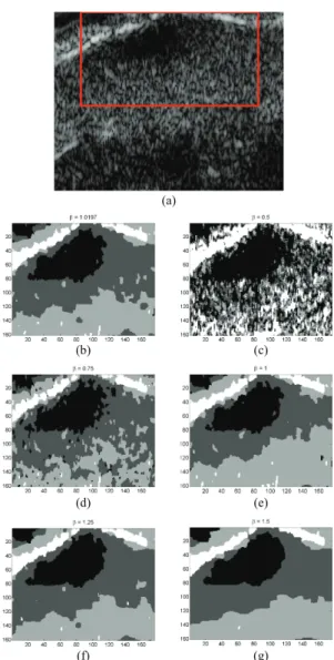
Fig. 6(a) shows a 3D B-mode ultrasound image of a skin lesion, acquired at 100MHz with a focalized 25MHz 3D probe (the lesion is contained within the region of interest (ROI) outlined by the red rectangle). Fig. 6(b) presents one slice
(a)
(b) (c)
(d) (e)
(f) (g)
Fig. 6. (a) Log-compressed US images of skin lesion and the cor-responding estimated class labels (lesion = black, epidermis = white, pap. dermis =dark gray, ret. dermis = light gray). MAP estimates of the class labels. (b) Results obtained r with the proposed method. (c)-(g) Results obtained with the algorithm [18] for β=(0.5, 0.75, 1, 1.25, 1.5).
of the 3D MAP label vector obtained with the proposed method. The MMSE estimate of the granularity coefficient corresponding to this result is ˆβ = 1.02 ± 0.07. To assess the influence of β, Figs. 6(c)–(g) show the MAP class labels obtained with the algorithm proposed in [18] for different values of β. Labels have been computed from a single Markov chain of T = 12 000 iterations whose first 2 000 iterations (burn-in period) have been removed. Precisely, these estimates have been computed individually for each voxel by calculating the mode of the discrete samples z(t )n (t = 2 000, . . . , T ).
Finally, computing these estimates required 316 minutes when estimating labels jointly with β and approximated 180 minutes when β was fixed.
Experts from the Hospital of Toulouse and Pierre Fabre Labs have found that the proposed method produces the most clear segmentation, that not only sharply locates the lesion but also provides realistic boundaries for the healthy skin layers
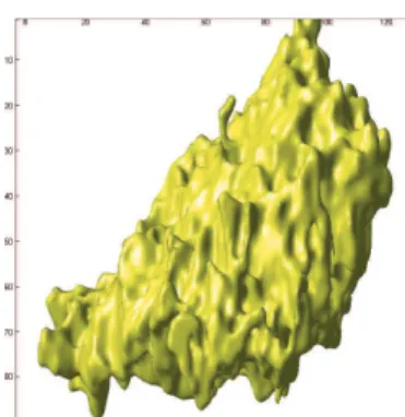
Fig. 7. Frontal viewpoint of a 3D reconstruction of the skin lesion.
within the region of interest. According to them, this result indicates that the lesion, which is known to have originated at the dermis-epidermis junction, has already invaded the upper half of the papillary dermis. Experts have also pointed out that the results obtained by fixing β to a small value were corrupted by ultrasound speckle noise and failed to capture the different skin layers. On the other hand, choosing a too large value of β enforces excessive spatial correlation and yields a segmentation with artificially smooth boundaries. It should be stressed that unlike man-made structures, skin tissues are very irregular and interpenetrate each other at the boundaries. Finally, Fig. 7 shows a frontal viewpoint of a 3D reconstruction of the lesion surface. We observe that the tumor has a semi-ellipsoidal shape which is cut at the upper left by the epidermis-dermis junction. The tumor grows from this junction towards the deeper dermis, which is at the lower right.
VII. CONCLUSION
This paper presented a hybrid Gibbs sampler for estimating the Potts parameter β jointly with the unknown parameters of a Bayesian segmentation model. In most image processing applications this important parameter is set heuristically by cross-validation. Standard MCMC methods cannot be applied to this problem because performing inference on β requires computing the intractable normalizing constant of the Potts model. In this work the estimation of β has been included within an MCMC method using an ABC likelihood-free Metropolis-Hastings algorithm, in which intractable terms have been replaced by simulation-rejection schemes. The ABC distance function has been defined using the Potts potential, which is the natural sufficient statistic for the Potts model. The proposed method can be applied to large images both in 2D and 3D scenarios. Experimental results obtained for synthetic data showed that estimating β jointly with the other unknown parameters leads to estimation results that are as good as those obtained with the actual value of β. On the other hand, choosing an incorrect value of β can degrade the estimation performance significantly. Finally, the proposed algorithm was successfully applied to real bidimensional SAR and tridimensional ultrasound images.
This study assumed that the number of classes K is known. Future work could relax this assumption by studying the esti-mation of β within a reversible jump MCMC algorithm [62], [63], or using the non-parametric approach presented in [64].
Alternatively, one could also apply the proposed method using different fixed values of K and then perform model choice to determine which value of K produced the best results [51]. Other prospects for future work include the development of a stochastic EM method where θ and z are updated determinis-tically while β is sampled using the proposed ABC algorithm. The application of the proposed method to estimate β within the hyperspectral image unmixing method proposed in [17] is currently under investigation.
ACKNOWLEDGMENT
The authors would like to thank the CNES, which provided the SAR and optical images used in Section VI-A. The authors are also grateful to the Hospital of Toulouse and Pierre Fabre Laboratories for the corpus of US images used in Section VI-B. Finally, they would like to thank the reviewers for their helpful comments.
REFERENCES
[1] S. Geman and D. Geman, “Stochastic relaxation, Gibbs distributions, and the Bayesian restoration of images,” IEEE Trans. Pattern Anal. Mach. Intell., vol. 6, no. 6, pp. 721–741, Nov. 1984.
[2] S. Z. Li, Markov Random Field Modeling in Image Analysis. New York, USA: Springer-Verlag, 2001.
[3] L. Cordero-Grande, G. Vegas-Sanchez-Ferrero, P. Casaseca-de-la Higuera, and C. Alberola-Lopez, “A Markov random field approach for topology-preserving registration: Application to object-based tomo-graphic image interpolation,” IEEE Trans. Image Process., vol. 21, no. 4, pp. 2047–2061, Apr. 2012.
[4] D. Mahapatra and Y. Sun, “Integrating segmentation information for improved MRF-based elastic image registration,” IEEE Trans. Image Process., vol. 21, no. 1, pp. 170–183, Jan. 2012.
[5] T. Katsuki, A. Torii, and M. Inoue, “Posterior mean super-resolution with a causal Gaussian Markov random field prior,” IEEE Trans. Image Process., vol. 21, no. 4, pp. 2187–2197, Apr. 2012.
[6] S. Jain, M. Papadakis, S. Upadhyay, and R. Azencott, “Rigid motion invariant classification of 3-D textures,” IEEE Trans. Image Process., vol. 21, no. 5, pp. 2449–2463, May 2012.
[7] H. Ayasso and A. Mohammad-Djafari, “Joint NDT image restoration and segmentation using Gauss–Markov–Potts prior models and variational Bayesian computation,” IEEE Trans. Image Process., vol. 19, no. 9, pp. 2265–2277, Sep. 2010.
[8] H. Snoussi and A. Mohammad-Djafari, “Fast joint separation and segmentation of mixed images,” J. Electron. Imag., vol. 13, no. 2, pp. 349–361, 2004.
[9] L. Risser, J. Idier, P. Ciuciu, and T. Vincent, “Fast bilinear extrapolation of 3D ising field partition function. Application to fMRI image analysis,” in Proc. IEEE Int. Conf. Image Proc., Nov. 2009, pp. 833–836. [10] L. Risser, T. Vincent, J. Idier, F. Forbes, and P. Ciuciu, “Min-max
extrapolation scheme for fast estimation of 3D Potts field partition functions. Application to the joint detection-estimation of brain activity in fMRI,” J. Sig. Proc. Syst., vol. 65, no. 3, pp. 325–338, Dec. 2011. [11] C. McGrory, D. Titterington, R. Reeves, and A. Pettitt, “Variational
Bayes for estimating the parameters of a hidden Potts model,” Stat. Comput., vol. 19, no. 3, pp. 329–340, Sep. 2009.
[12] S. Pelizzari and J. Bioucas-Dias, “Oil spill segmentation of SAR images via graph cuts,” in Proc. IEEE Int. Geosci. Remote Sens. Symp., Jul. 2017, pp. 1318–1321.
[13] M. Picco and G. Palacio, “Unsupervised classification of SAR images using Markov random fields and G0I model,” IEEE Trans. Geosci. Remote Sens., vol. 8, no. 2, pp. 350–353, Mar. 2011.
[14] M. Mignotte, “Image denoising by averaging of piecewise constant simulations of image partitions,” IEEE Trans. Image Process., vol. 16, no. 2, pp. 523–533, Feb. 2007.
[15] M. Mignotte, “A label field fusion Bayesian model and its penalized maximum rand estimator for image segmentation,” IEEE Trans. Image Process., vol. 19, no. 6, pp. 1610–1624, Jun. 2010.
[16] K. Kayabol, E. Kuruoglu, and B. Sankur, “Bayesian separation of images modeled with MRFs using MCMC,” IEEE Trans. Image Process., vol. 18, no. 5, pp. 982–994, May 2009.
[17] O. Eches, N. Dobigeon, and J.-Y. Tourneret, “Enhancing hyperspectral image unmixing with spatial correlations,” IEEE Trans. Geosci. Remote Sens., vol. 49, no. 11, pp. 4239–4247, Nov. 2011.
[18] M. Pereyra, N. Dobigeon, H. Batatia, and J.-Y. Tourneret, “Segmentation of skin lesions in 2-D and 3-D ultrasound images using a spatially coherent generalized Rayleigh mixture model,” IEEE Trans. Med. Imag., vol. 31, no. 8, pp. 1509–1520, Aug. 2012.
[19] X. Descombes, R. Morris, J. Zerubia, and M. Berthod, “Estimation of Markov random field prior parameters using Markov chain Monte Carlo maximum likelihood,” IEEE Trans. Image Process., vol. 8, no. 7, pp. 945–963, Jun. 1999.
[20] I. Murray and Z. Ghahramani, “Bayesian learning in undirected graph-ical models: Approximate MCMC algorithms,” in Proc. 20th Conf. Uncertainty Artif. Intell., 2004, pp. 392–399.
[21] Y. Cao, H. Sun, and X. Xu, “An unsupervised segmentation method based on MPM for SAR images,” IEEE Trans. Geosci. Remote Sens., vol. 2, no. 1, pp. 55–58, Jan. 2005.
[22] J. Besag, “Statistical analysis of non-lattice data,” J. Roy. Stat. Soc. Ser. D, vol. 24, no. 3, pp. 179–195, Sep. 1975.
[23] C. J. Geyer and E. A. Thompson, “Constrained Monte Carlo maximum likelihood for dependent data (with discussions),” J. Roy. Statist. Soc., vol. 54, no. 3, pp. 657–699, Apr. 1992.
[24] G. Celeux, F. Forbes, and N. Peyrard, “EM procedures using mean field-like approximations for Markov model-based image segmentation,” Pattern Recognit., vol. 36, no. 1, pp. 131–144, Jan. 2003.
[25] F. Forbes and N. Peyrard, “Hidden Markov random field selection criteria based on mean field-like approximations,” IEEE Trans. Patt. Anal. Mach. Intell., vol. 25, no. 8, pp. 1089–1101, Aug. 2003. [26] F. Forbes and G. Fort, “Combining Monte Carlo and mean field like
methods for inference in hidden Markov random fields,” IEEE Trans. Image Process., vol. 16, no. 3, pp. 824–837, Mar. 2007.
[27] C. P. Robert and G. Casella, Monte Carlo Statistical Methods, 2nd ed. New York, USA: Springer-Verlag, 2004.
[28] A. Gelman and X. Meng, “Simulating normalizing constants: From importance sampling to bridge sampling to path sampling,” Statist. Sci., vol. 13, no. 2, pp. 163–185, Nov. 1998.
[29] M. Pereyra, N. Dobigeon, H. Batatia, and J.-Y. Tourneret, “Estimat-ing the granularity parameter of a Potts-Markov random field within an MCMC algorithm,” Dept. IRIT/INP-ENSEEIHT, Univ. Toulouse, Toulouse, France, Tech. Rep., Feb. 2012.
[30] J. Moller, A. N. Pettitt, R. Reeves, and K. K. Berthelsen, “An efficient Markov chain Monte Carlo method for distributions with intractable nor-malising constants,” Biometrika, vol. 93, no. 2, pp. 451–458, Jun. 2006. [31] C. Andrieu, A. Doucet, and R. Holenstein, “Particle Markov chain Monte Carlo methods,” J. Roy. Stat. Soc. Ser. B, vol. 72, no. 3, pp. 1–76, May 2010.
[32] P. Del Moral, A. Doucet, and A. Jasra, “Sequential Monte Carlo samplers,” J. Roy. Stat. Soc. Ser. B, vol. 68, no. 3, pp. 411–436, Jun. 2006.
[33] I. Murray, Z. Ghahramani, and D. MacKay, “MCMC for doubly-intractable distributions,” in Proc. 22nd Annu. Conf. Uncertainty Artif. Intell., Jul. 2006, pp. 359–366.
[34] R. G. Everitt, “Bayesian parameter estimation for latent Markov random fields and social networks,” J. Comput. Graph. Stat., vol. 21, no. 4, pp. 1–27, Mar. 2012.
[35] P. Marjoram, J. Molitor, V. Plagnol, and S. Tavaré, “Markov chain Monte Carlo without likelihoods,” Proc. Nat. Acad. Sci., vol. 100, no. 26, pp. 15324–15328, Dec. 2003.
[36] J.-M. Marin, P. Pudlo, C. P. Robert, and R. Ryder, “Approximate Bayesian computational methods,” Stat. Comput., vol. 21, no. 2, pp. 289–291, Oct. 2011.
[37] R. Kindermann and J. L. Snell, Markov Random Fields and Their Applications. Providence, RI, USA: AMS, 1980.
[38] X. Descombes, F. Kruggel, and D. Von Cramon, “Spatio-temporal fMRI analysis using Markov random fields,” IEEE Trans. Med. Imag., vol. 17, no. 6, pp. 1028–1039, Dec. 1998.
[39] F. Y. Wu, “The Potts model,” Rev. Mod. Phys., vol. 54, no. 1, pp. 235–268, Jan. 1982.
[40] T. Vincent, L. Risser, and P. Ciuciu, “Spatially adaptive mixture model-ing for analysis of fMRI time series,” IEEE Trans. Med. Imag., vol. 29, no. 4, pp. 1059–1074, Apr. 2010.
[41] K. Kayabol, E. Kuruoglu, J. Sanz, B. Sankur, E. Salerno, and D. Herranz, “Adaptive Langevin sampler for separation of t-distribution modelled astrophysical maps,” IEEE Trans. Image Process., vol. 19, no. 9, pp. 2357–2368, Sep. 2010.
[42] X. Zhou, Y. Lu, J. Lu, and J. Zhou, “Abrupt motion tracking via intensively adaptive Markov-chain Monte Carlo sampling,” IEEE Trans. Image Process., vol. 21, no. 2, pp. 789–801, Feb. 2012.
[43] F. Destrempes, J.-F. Angers, and M. Mignotte, “Fusion of hidden Markov random field models and its Bayesian estimation,” IEEE Trans. Image Process., vol. 15, no. 10, pp. 2920–2935, Oct. 2006.
[44] C. Nikou, A. Likas, and N. Galatsanos, “A Bayesian framework for image segmentation with spatially varying mixtures,” IEEE Trans. Image Process., vol. 19, no. 9, pp. 2278–2289, Sep. 2010.
[45] F. Orieux, E. Sepulveda, V. Loriette, B. Dubertret, and J.-C. Olivo-Marin, “Bayesian estimation for optimized structured illumination microscopy,” IEEE Trans. Image Process., vol. 21, no. 2, pp. 601–614, Feb. 2012.
[46] A. P. Dempster, N. M. Laird, and D. B. Rubin, “Maximum likelihood from incomplete data via the EM algorithm,” J. Roy. Stat. Soc. Ser. B, vol. 39, no. 1, pp. 1–38, 1977.
[47] N. Bali and A. Mohammad-Djafari, “Bayesian approach with hidden Markov modeling and mean field approximation for hyperspectral data analysis,” IEEE Trans. Image Process., vol. 17, no. 2, pp. 217–225, Feb. 2008.
[48] J. Gonzalez, Y. Low, A. Gretton, and C. Guestrin, “Parallel Gibbs sampling: From colored fields to thin junction trees,” in Proc. Artif. Intell. Stat., May 2011, pp. 324–332.
[49] J. G. Propp and D. B. Wilson, “Exact sampling with coupled Markov chains and applications to statistical mechanics,” Rand. Struct. Algo-rithms, vol. 9, nos. 1–2, pp. 223–252, Aug.–Sep. 1996.
[50] A. M. Childs, R. B. Patterson, and D. J. C. MacKay, “Exact sampling from nonattractive distributions using summary states,” Phys. Rev. E, vol. 63, no. 3, pp. 36113–36118, Feb. 2001.
[51] A. Grelaud, J. M. Marin, C. Robert, F. Rodolphe, and F. Tally, “Likelihood-free methods for model choice in Gibbs random fields,” Bayesian Anal., vol. 3, no. 2, pp. 427–442, Jan. 2009.
[52] F. Liang, “A double Metropolis-hastings sampler for spatial models with intractable normalizing constants,” J. Stat. Comp. Simul., vol. 80, no. 9, pp. 1007–1022, 2010.
[53] M. A. Beaumont, W. Zhang, and D. J. Balding, “Approximate Bayesian computation in population genetics,” Genetics, vol. 162, no. 4, pp. 2025–2035, 2002.
[54] C. P. Robert and S. Richardson, “Markov chain Monte Carlo methods,” in Discretization and MCMC Convergence Assessment, C. P. Robert, Ed. New York, USA: Springer-Verlag, 1998, pp. 1–25.
[55] J.-Y. Tourneret, M. Doisy, and M. Lavielle, “Bayesian retrospective detection of multiple changepoints corrupted by multiplicative noise. Application to SAR image edge detection,” Signal Process., vol. 83, no. 9, pp. 1871–1887, Sep. 2003.
[56] M. A. Pereyra and H. Batatia, “Modeling ultrasound echoes in skin tissues using symmetric α-stable processes,” IEEE Trans. Ultrason. Ferroelect. Freq. Contr., vol. 59, no. 1, pp. 60–72, Jan. 2012.
[57] E. Kuruoglu and J. Zerubia, “Modeling SAR images with a generaliza-tion of the Rayleigh distribugeneraliza-tion,” IEEE Trans. Image Process., vol. 13, no. 4, pp. 527–533, Apr. 2004.
[58] A. Achim, E. Kuruoglu, and J. Zerubia, “SAR image filtering based on the heavy-tailed Rayleigh model,” IEEE Trans. Image Process., vol. 15, no. 9, pp. 2686–2693, Sep. 2006.
[59] C. Tison, J.-M. Nicolas, F. Tupin, and H. Maitre, “A new statistical model for Markovian classification of urban areas in high-resolution SAR images,” IEEE Trans. Geosci. Remote Sens., vol. 42, no. 10, pp. 2046–2057, Oct. 2004.
[60] H. Deng and D. Clausi, “Unsupervised segmentation of synthetic aperture radar sea ice imagery using a novel Markov random field model,” IEEE Trans. Geosci. Remote Sens., vol. 43, no. 3, pp. 528–538, Mar. 2005.
[61] Y. Li, J. Li, and M. Chapman, “Segmentation of SAR intensity imagery with a Voronoi tessellation, Bayesian inference, and reversible jump MCMC algorithm,” IEEE Trans. Geosci. Remote Sens., vol. 48, no. 4, pp. 1872–1881, Apr. 2010.
[62] P. J. Green, “Reversible jump Markov chain Monte Carlo methods computation and Bayesian model determination,” Biometrika, vol. 82, no. 4, pp. 711–732, Dec. 1995.