Impact of spatial data resolution on simulated catchment water balances and model performance of the multi-scale TOPLATS model

(1)

HAL Id: hal-00304833

https://hal.archives-ouvertes.fr/hal-00304833

Submitted on 3 Mar 2006

HAL is a multi-disciplinary open access

archive for the deposit and dissemination of

sci-entific research documents, whether they are

pub-lished or not. The documents may come from

teaching and research institutions in France or

abroad, or from public or private research centers.

L’archive ouverte pluridisciplinaire HAL, est

destinée au dépôt et à la diffusion de documents

scientifiques de niveau recherche, publiés ou non,

émanant des établissements d’enseignement et de

recherche français ou étrangers, des laboratoires

publics ou privés.

catchment water balances and model performance of the

multi-scale TOPLATS model

H. Bormann

To cite this version:

H. Bormann. Impact of spatial data resolution on simulated catchment water balances and model

performance of the multi-scale TOPLATS model. Hydrology and Earth System Sciences Discussions,

European Geosciences Union, 2006, 10 (2), pp.165-179. �hal-00304833�

(2)

Earth System

Sciences

Impact of spatial data resolution on simulated catchment water

balances and model performance of the multi-scale TOPLATS

model

H. Bormann

University of Oldenburg, Department of biology and environmental sciences, Uhlhornsweg 84, 26 111 Oldenburg, Germany Received: 30 August 2005 – Published in Hydrol. Earth Syst. Sci. Discuss.: 10 October 2005

Revised: 16 January 2006 – Accepted: 18 January 2006 – Published: 3 March 2006

Abstract. This paper analyses the effect of spatial input data resolution on the simulated water balances and flow compo-nents using the multi-scale hydrological model TOPLATS. A data set of 25 m resolution of the central German Dill

catch-ment (693 km2) is used for investigation. After an

aggrega-tion of digital elevaaggrega-tion model, soil map and land use classi-fication to 50 m, 75 m, 100 m, 150 m, 200 m, 300 m, 500 m, 1000 m and 2000 m, water balances and water flow compo-nents are calculated for the entire Dill catchment as well as for 3 subcatchments without any recalibration. The study shows that model performance measures and simulated water balances almost remain constant for most of the aggregation steps for all investigated catchments. Slight differences in the simulated water balances and statistical quality measures oc-cur for single catchments at the resolution of 50 m to 500 m (e.g. 0–3% for annual stream flow), significant differences at the resolution of 1000 m and 2000 m (e.g. 2–12% for annual stream flow). These differences can be explained by the fact that the statistics of certain input data (land use data in partic-ular as well as soil physical characteristics) changes signifi-cantly at these spatial resolutions. The impact of smoothing the relief by aggregation occurs continuously but is barely reflected by the simulation results. To study the effect of aggregation of land use data in detail, in addition to current land use the effect of aggregation on the water balance cal-culations based on three different land use scenarios is inves-tigated. Land use scenarios were available aiming on eco-nomic optimisation of agricultural and forestry practices at different field sizes (0.5 ha, 1.5 ha and 5.0 ha). The changes in water balance terms, induced by aggregation of the land use scenarios, are comparable with respect to catchment wa-ter balances compared to the current land use. A correlation analysis between statistics of input data and simulated an-nual water fluxes only in some cases reveals systematically

Correspondence to: H. Bormann

(helge.bormann@uni-oldenburg.de)

high correlation coefficients for all investigated catchments and data sets (e.g. actual evapotranspiration is correlated to land use, surface runoff generation is correlated to soil prop-erties). Predominantly the correlation between catchment properties (e.g. topographic index, transmissivity, land use) and simulated water flows varies from catchment to catch-ment. Catchment specific properties determine correlations between properties and fluxes, but do not influence the effect of data aggregation. This study indicates that an aggregation of input data for the calculation of regional water balances using TOPLATS type models leads to significant errors from a resolution exceeding 500 m. Correlating statistics of input data and simulation results indicates that a meaningful aggre-gation of data should in the first instance aim on preserving the areal fractions of land use classes.

1 Introduction

Many recent environmental problems such as non-point source pollution and habitat degradation are addressed at basin scale (e.g. the “Water Framework Directive” of the Eu-ropean Union, EU-WFD, 2000) and require spatially explicit analyses and predictions. Especially future predictions have to be based on model applications to simulate future condi-tions of ecosystems in catchments and the effects of environ-mental change. As the water flow is essential for transport of nutrients and pollutants as well as the development of habi-tats, distributed modelling of water flows and related state variables is a pre-requisite to contribute to the solution of these environmental problems.

Spatially distributed modelling of regional water fluxes and water balances requires a number of huge spatial data sets. At least spatial information on topography (digital el-evation model), soils and vegetation is needed. Thereby the higher the resolution of these data is the better the landscape is represented by the data base (Kuo et al., 1999). Spatial

(3)

patterns can be represented more in detail and small scale fluxes can be considered by the models.

But a higher spatial and temporal resolution of data and model application does not always lead to a better represen-tation of the water fluxes for a given catchment. This de-pends on the spatiotemporal variability and the spatial dis-tribution of catchment properties. Varying spatial resolution can also have effects on response times of catchments. And spatial discretisation may influence model sensitivity at dif-ferent scales by varying consideration of climatological vari-ability. For example Andreassian et al. (2001) found that imperfect rainfall knowledge can reduce the consistency of catchment model parameters.

Despite a better representation of the landscape highly re-solved data often contain redundant information and lead to an increase in required storage capacity and computer time (Omer et al., 2003). And, of course, highly resolved data are not always available for every catchment of interest. There-fore new initiatives search for new ways to better represent the catchment water fluxes in poor data situations. One well known example is the PUB initiative (prediction of ungauged basins) of the International Association of Hydrological Sci-ences (Sivapalan et al., 2003).

Furthermore the benefit of a detailed data base strongly depends on the model type applied and on the target of a

study. Focusing on annual water balances of large scale

catchments, for instance, does not require diurnal input data at micro-scale resolution. And lumped, conceptual models do not exploit highly resolved data in the same way as spa-tially distributed and process based models do. Therefore the decision, which data resolution to be sufficient for a distinct model application, has to be made again for every case study. As it is very time-consuming and costly to perform this anal-ysis, unfortunately it is not made for each study. Based on experience of the user and data availability, the appropriate data resolution is chosen for a given scale and a given tar-get. But the impact of spatial resolution on simulation results mostly is not investigated.

A few studies have examined the effect of grid size of to-pographic input data on catchment simulations using TOP-MODEL (Beven et al., 1995). Quinn et al. (1991), Moore et al. (1993), Zhang and Montgomery (1994), Bruneau et al. (1995) and Wolock and Price (1994) looked at how grid size affected the computed topographic characteristics, wet-ness index and outflow. In general, they found that higher resolved grids gave better results. Kuo et al. (1999) applied a variable sources area model to grid sizes from 10 to 600 m and revealed an increasing misrepresentation of the curva-ture of the landscape with increasing grid size while soil properties and land use distribution were not affected. Ef-fects themselves depended on the wetness of the time peri-ods considered. Thieken et al. (1999) examined the effect of differently sized elevation data sets on catchment charac-teristics and calculated hydrographs of single events. They found that these data sets with a resolution between 10 and

50 m strongly diverged in landscape representation. Further-more these differences in topographic and geomorphologic features could be used to explain differences in the runoff simulation of single events. The effect on long-term water balances was not investigated. Farajalla and Vieux (1995) showed that the aggregation of spatial input data led to a de-crease in entropy of soil hydraulic parameters between 200 m and 600 m grid size and to a significant decrease for grid sizes over 1000 m. To overcome the problem of information loss with increasing grid size Beven (1995) suggests the consid-eration of subgrid variability by spatial distribution functions of properties or parameters. This only works if high resolu-tion data sets are available. Model concepts which are based on Hydrological Response Units (HRUs) instead of grid cells are faced with the same problem. For that reason the ef-fect of a decreasing number of HRUs on the simulation re-sults was investigated by various authors, too (e.g. Chen and Mackay, 2004; Lahmer et al., 2000; Bormann et al., 1999). They found that a minimum number of HRUs is required to represent the variability in catchment properties while fur-ther increasing of computational units does not improve the simulation results significantly. Boiij (2005) compared three spatial resolutions comparing the conceptual HBV-model to the Meuse river (1, 15, and 118 subcatchments). The model results after individual calibration at all resolutions showed that all models reproduced well the average and the extremes, while increasing the resolution slightly improved the model results. Skøien and Bl¨oschl (2003) analysed characteristic space scales more in general by performing a variogramm analysis on hydrological fluxes (precipitation, runoff) and

state variables (groundwater tables, soil moisture). They

found that the variance of stream flow increases faster with decreasing catchment size than with the inverse of catchment area which can be interpreted as an indicator for spatial or-ganisation. Information on spatial organisation disappears with increased data aggregation. But they also found char-acteristic space scales in the order of 8 km to 60 km which is much larger than the model resolution investigated in this study. So these characteristic space scales should not limit the results obtained in this study.

Although it is well reported in literature that data resolu-tion can have a significant impact on the simularesolu-tion results, model results of different models often are compared and evaluated without taking the basic data resolution into ac-count. Therefore this study elaborates in detail, which effect the chosen data and model resolution can have on model per-formance and simulated water balances considering all spa-tial data sets required. Based on a detailed spaspa-tial data set

(25m resolution) of the meso-scale Dill catchment (693 km2)

in central Germany a systematic data aggregation (from 25 m to 2000 m) and subsequent model application is carried out to investigate the limitations of data aggregation and model ap-plicability in case of the TOPLATS model (Famiglietti and Wood, 1994a). The study aims on the calculation of water balances, therefore effects of aggregation on response times

(4)

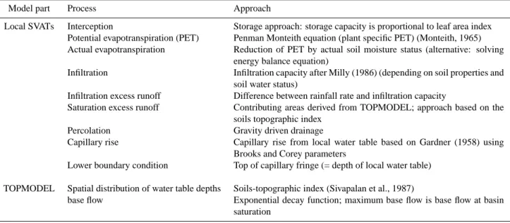
Table 1. Main processes and equations of the TOPLATS model.

Model part Process Approach

Local SVATs Interception Storage approach: storage capacity is proportional to leaf area index

Potential evapotranspiration (PET) Penman Monteith equation (plant specific PET) (Monteith, 1965) Actual evapotranspiration Reduction of PET by actual soil moisture status (alternative: solving

energy balance equation)

Infiltration Infiltration capacity after Milly (1986) (depending on soil properties and

soil water status)

Infiltration excess runoff Difference between rainfall rate and infiltration capacity

Saturation excess runoff Contributing areas derived from TOPMODEL; approach based on the

soils topographic index

Percolation Gravity driven drainage

Capillary rise Capillary rise from local water table based on Gardner (1958) using

Brooks and Corey parameters

Lower boundary condition Top of capillary fringe (= depth of local water table) TOPMODEL Spatial distribution of water table depths Soils-topographic index (Sivapalan et al., 1987)

base flow Exponential decay function; maximum base flow is base flow at basin

saturation

do not play a major role. The potential influence of grid size dependent rainfall variability was excluded by using the same weather inputs for the simulations on different grid sizes. The influence of the aggregation of the spatial input data sets such as land use, topography and soils is additionally inves-tigated by analysing correlation coefficients between input data and simulation results. To further explore the effect of differently structured land cover three land use scenarios are aggregated and studied supplementary.

The motivation for this study arose from a model compar-ison initiative (LUCHEM initiative, “Assessing the impact of land use change on hydrology by ensemble modelling”, initi-ated by the working group on “Resources Management of the University of Gießen, Germany”) where different catchment models were compared despite differences in process repre-sentation, spatial conceptualisation (grid, HRUs) and spatial resolution in a relatively tight range (25 m–200 m). There the question of the influence of grid size on simulation results arose.

2 Material and methods

2.1 Toplats model

The TOPLATS model (“TOPMODEL based atmosphere transfer scheme”; Famiglietti and Wood, 1994a; Peter-Lidard et al., 1997) is a multi-scale model to simulate local to re-gional scale catchment water fluxes. It combines a “soil veg-etation atmosphere transfer scheme” (SVAT) to represent lo-cal slo-cale vertilo-cal water fluxes with the catchment slo-cale TOP-MODEL approach (Beven et al., 1995) to laterally redis-tribute the water within a catchment.

TOPLATS is a grid based and time continuous model. The vertical water fluxes of the grid cells are calculated by the lo-cal SVATs (Fig. 1). Catchment slo-cale vertilo-cal water fluxes are obtained by aggregation of local water fluxes. There is no lateral interaction between the local SVATs accounted for by the model. But based on the soils topographic index of the TOPMODEL approach (Beven et al., 1995), a lateral redistri-bution of water is realized by adaptation of the local ground-water levels which are used as lower boundary conditions of the local SVATs. Finally, based flow is generated from the in-tegration of local saturated subsurface fluxes along the chan-nel network. A routing routine is not integrated in the model. The basic hydrological processes and their representation in the TOPLATS model are summarized in Table 1.

In vertical direction the soil is divided in 2 layers (root

zone and transmission zone). According to Sivapalan et

al. (1987) it is assumed that saturated conductivity exponen-tially decreases with depth. The percolation is calculated us-ing an approximation for gravity driven drainage, and cap-illary rise is calculated based on the approach of Gardner (1958), both approaches using the Brooks and Corey pa-rameterisation of soil retention characteristics (Brooks and Corey, 1964). Based on soil texture and porosity soil param-eters are derived using the pedotransfer-function of Rawls and Brakensiek (1985). Plant growth is not directly simu-lated by TOPLATS, but the seasonal development of plant properties is described by monthly updating the plant param-eter sets consisting of e.g. leaf area index, plant height and stomatal resistance. Plant parameters were taken from the PlaPaDa data base (Breuer et al., 2003). The digital elevation model serves as basic data set for the calculation of the topo-graphic wetness index (Beven et al., 1995), which is used for

(5)

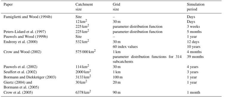
Table 2. Scale relevant characteristics of TOPLATS model applications in literature. “Parameter distribution function” refers to the statistical

mode of TOPLATS considering spatial variability of basin properties by a parameter distribution function (Famiglietti and Wood, 1994a). The statistical mode was not used in this study.

Paper Catchment size Grid size Simulation period

Famiglietti and Wood (1994b) Site

12 km2 225 km2

– 30 m

parameter distribution function

Days Days 3 weeks

Peters-Lidard et al. (1997) 225 km2 parameter distribution function 5 months

Pauwels and Wood (1999b) Site – 1 year

Endreny et al. (2000) 532 km2 30 m

60 index values

12 days 10 years

Crow and Wood (2002) 575 000 km2 1 km

parameter distribution functions for 314 subcatchents

4 months 39 months

Pauwels et al. (2002) 114 km2 30 m 4 years

Seuffert et al. (2002) 2000 km2 1 km 3 years

Bormann and Diekkr¨uger (2003) 3133 km2 100 m 1 year

Giertz (2004) and Bormann et al. (2005)

30 km2 20 m 1 year

Crow et al. (2005) 6378 km2 90 m 1 month

calculation of the soils-topographic index (see Table 1) ad-ditionally accounting for local differences in transmissivity (Sivapalan et al., 1987). For further details about the model the reader is referred to Famiglietti and Wood (1994a) and Peters-Lidard et al. (1997).

The TOPLATS model has been successfully applied in several studies at different scales (Table 2) and in different climate regions around the world. Famiglietti and Wood (1994b) applied TOPLATS to the tallgrass prairie in the United States. They applied TOPLATS to single sites and

a small catchment (12 km2)and simulated diurnal variations

of water fluxes up to a couple of weeks to be able to compare simulations to evapotranspiration measurements. Pauwels and Wood (1999a, b) extended the TOPLATS model to the application in high latitudes in Canada. They also focused on small scale simulations (sites) but simulated water and energy fluxes for whole seasons.

Recent TOPLATS related publications more and more fo-cus on regional applications and on the integration of re-motely sensed data to improve the simulations. Endreny et al. (2000) examined the effects of the errors induced by the use of digital elevation models derived from SPOT data and compared the simulation results to those based on standard data sets (USGS 7.5-min data set). Analysing the effects of the accuracy of the digital elevation model on simulated water fluxes he implicitly also investigated the aggregation effect. It can be assumed that accuracy of the digital ele-vation model decreases with increasing grid size as the sur-face is smoothed. Seuffert et al. (2002) coupled TOPLATS to an atmospheric model (“Lokal-Modell” of the German

Me-teorological Service) and applied the model to the regional

scale Sieg catchment (about 2000 km2)in Western Germany.

Pauwels et al. (2002) investigated the possibility to improve TOPLATS based simulation by the use of ERS derived soil moisture values at the catchment scale. A similar study was performed by Crow and Wood (2002) in the Red Arkansas basin who explored the benefit of coarse-scale soil mois-ture images for macro-scale model applications of TOPLATS

(575 000 km2). And Crow et al. (2005) also examined the

possibility to upscale field-scale soil moisture measurements by means of distributed land surface modelling. In the con-text of this study they also expanded the soil module within TOPLATS considering vertical soil heterogeneity. Finally Bormann and Diekkr¨uger (2003), Giertz (2004) and Bor-mann et al. (2005) applied TOPLATS to the subhumid trop-ics of West Africa to simulate seasonal dynamtrop-ics stream flow and soil moisture. They found that TOPLATS reproduced spatial patterns of soil moisture and seasonal dynamics in stream flow on the local scale driven by local mapping cam-paigns. Based on poor data neither on local nor on regional scale TOPLATS could reproduce the hydrological behaviour of the catchments as physiographic variability was not cov-ered by the data. Therefore applicability of TOPLATS in the subhumid tropics seems to be limited by input data availabil-ity.

Recapitulating TOPLATS has successfully been applied to a wide range of temporal and spatial scales in different cli-mate regions (Table 2). Analysing the scale relevant char-acteristics of the cited model applications it can be observed that model applications range from site scale to macroscale,

(6)

lateral subsurface flow capillary fringe transmission zone root zone percolation surface runoff infiltration evaporation percolation capillary rise radiation transpiration & interception precipitation throughfall leaf drip

Fig. 1. Hydrological processes of the local SVATs represented by

the TOPLATS model (modified after Famiglietti and Wood, 1994a).

and grid sizes range from 20 m to 1 km. On the small catch-ment scale applications are run with small grid sizes while for large catchments also larger grid cells are used. This im-plicates constraints in data availability and in computational effort and underpins the necessity to investigate the effect of aggregation and increasing grid size on model results.

2.2 Catchment characteristics and available data sets of the

Dill basin

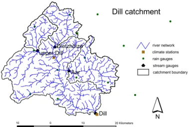
The Dill catchment (693 km2)is located in central Germany

and belongs to the Lahn-Dill low mountainous region. It is the target catchment of the SFB 299 (“Land use options for peripheral regions”) of the University of Gießen (Germany). Stream gauging stations exist for three sub-catchments

(Up-per Dill (63 km2), Dietzh¨olze (81 km2)and Aar (134 km2))

as well as for the entire Dill catchment at Asslar (693 km2,

Fig. 2).

The typical small scale topography ranges between 155 m and 674 m above sea level. The mean steepness of the slopes is approximately 14%. Mean annual rainfall ranges between 700 mm to 1100 mm depending on the location within the catchment and the corresponding elevation. Low precipita-tion areas show summer-dominated precipitaprecipita-tion and high precipitation areas winter-dominated precipitation regimes.

Average annual mean temperature is about 8◦C.

Soil parent material of the Lahn-Dill mountains is mainly argillaceous schist, greywacke, diabase, sandstone, quartzite,

; ; ; ; # # # # # # # # # # # # # # # # % [ % [ N ; # % [ Dill catchment river network climate stations rain gauges stream gauges catchment boundary 10 0 10 20 Kilometers Aar Dill upper Dill Dietzhölze

Fig. 2. Subcatchments (upper Dill, Dietzh¨olze, Aar), rain and stream gauges in the Dill catchment (693 km2)in central Germany.

and basalt which developed during the Devon and Lower Carbon. During the Pleistocene periglacial processes have

strongly influenced the soil parent material. Therefore

periglacial layers strongly influenced by the underlying geo-logic substrate are the main soil parent material of the catch-ment. Due to the heterogeneous nature of these periglacial layers, the pattern of soil types is complex. Main soil types are shallow cambisols, planosols derived from luvisols under hydromorphic conditions, and gleysols in groundwater influ-enced valleys.

Typical for most of the catchment area is a hard rock aquifer. Pore aquifers only exist in quaternary deposits such as river terraces or hillslope debris. Based on empirical rela-tions the portion of baseflow contribution to discharge can be estimated to an amount of 9–16%. Most of the discharge of the Dill river is delivered through interflow. The contribution of surface runoff is estimated to be less than 10%.

Current land cover of the Dill area is dominated by for-est. 29.5% of the catchment is covered by deciduous forest, 24.9% by coniferous forest. 20.5% of the catchment area is used for grassland and 6.5% agricultural crops. A portion of about 9% of the area is fallow land, and another 9% is cov-ered by urban area. Obviously the Dill catchment is a periph-eral region dominated by extensive agriculture and forestry. Thanks to the SFB 299 of the University of Gießen a detailed data base is available for the whole Dill basin at 25 m reso-lution. Spatial data sets and time series (rain gauges, climate stations and stream gauges, for location of the stations see Fig. 2) used in this study are summarised in Table 3.

2.3 Data aggregation

As the impact of increasing information loss on the calcu-lation of regional scale water fluxes was to be investigated by this study, the available data set of 25 m resolution was

(7)

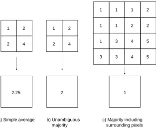
a) Simple average b) Unambiguous majority c) Majority including surrounding pixels 1 2 4 2 1 2 4 2 1 2 4 3 2.25 2 1 1 1 3 3 4 5 5 2 2 1 1 1

Fig. 3. Algorithms for systematic aggregation of spatial data sets:

simple average (a) for DEM aggregation, majority (b) for aggrega-tion of land use and soils, consideraaggrega-tion of the surrounding pixels if there is no unambiguous majority (c).

aggregated stepwise to create grid based data sets of increas-ing grid size: 50 m, 75 m, 100 m, 150 m, 200 m, 300 m,

500 m, 1 km, and 2 km. Therefore the spatial data sets

(soil map, DEM, land use classification, land use scenarios) were systematically aggregated applying standard aggrega-tion methods provided by standard GIS software.

The aggregation of the DEM was carried out by calculat-ing the arithmetic averages of the pixels to be aggregated. Concerning soils and land use the data sets were aggregated with respect to the majority of the pixels to be aggregated. The most frequent value was allocated to the aggregated pixel. If there was no unambiguous majority the surrounding pixels were included into the allocation (Fig. 3). Applying these algorithms, the DEM is smoothened by averaging, and the total area of small homogenous areas of classified data (soils, land use) decreases as small areas often disappear at the expense of large homogenous areas.

3 Model application to the Dill catchment

3.1 Calibration and validation

In order to reduce the calibration of the TOPLATS model for application to the Dill basin to a minimum, parameterisation of the TOPLATS model was carried out by deriving or using directly as many parameters as possible from standard data bases. Those parameters have not been touched during the calibration procedure. Thus transferability of the model and the obtained results to other catchments is improved. Cali-bration could be reduced to an adjustment of plant specific stomatal resistances by a constant factor to meet the long-term water balance and to the calibration of the parameters of the base flow recession curve. During the calibration process, two performance measures were applied. At first, calibration

aimed at the annual water balance of the whole Dill catch-ment to close the water balance of the model, and secondly the model efficiency according to Nash and Suttcliffe (1970) was optimised for daily resolution to reproduce the temporal variability of stream flow focusing on seasonal dynamics and short time variability. Applying these two quality measures, both long-term water balances and seasonal dynamics were covered well. Model calibration for the Dill catchment was carried out on the 50 m grid due to a limitation in the number of computational units within TOPLATS.

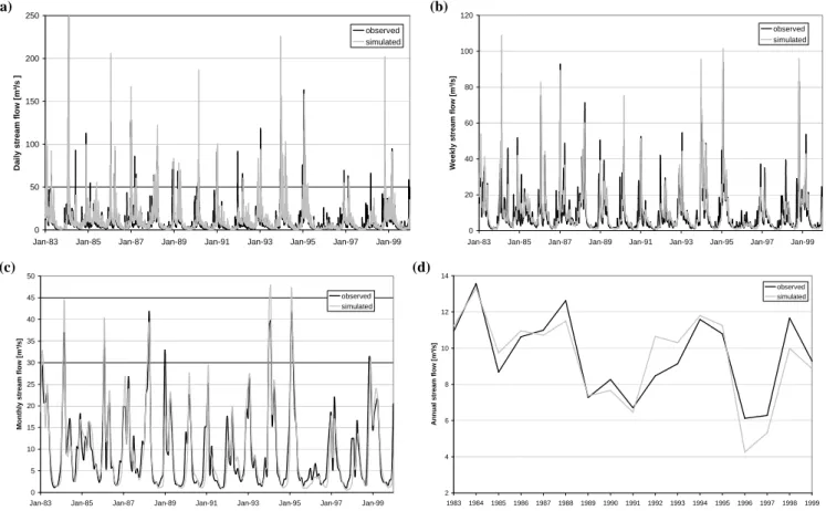
Figure 4 shows the simulation results for the entire Dill

catchment (693 km2)compared to the observed values of the

stream gauges. Calibration period is from 1983–1989, val-idation period from 1990–1999. The accuracy of the sim-ulation is satisfactory (quality measures see Table 4) con-sidering that TOPLATS was calibrated only with respect to stomatal resistance and the baseflow recession curve. Qual-ity measures for the validation period are only slightly worse than for the calibration period. While for daily discharges the model efficiency (Nash and Suttliffe, 1970) is of mod-erate quality (0.65 for calibration, 0.61 for validation), the model efficiencies and coefficients of determination increase for longer time intervals (longer than one week) to values greater than 0.8. The mean bias in discharge between obser-vations and simulations is about 5% for calibration and 12% for validation period.

For the simulation of the three subcatchments a recalibra-tion was not carried out except the maximum baseflow pa-rameter (baseflow at basin saturation). The simulation results

for the Dietzh¨olze (81 km2)and the upper Dill (63 km2)are

quite good while the results for the Aar catchment (134 km2)

are of a moderate quality. Model efficiencies for daily dis-charges range between 0.59 and 0.73 (calibration period) and between 0.52 and 0.69 (validation period). They in-crease with increasing time interval to values of 0.76 to 0.85 (weeks) and 0.82 to 0.90 (months). The values of the

coef-ficients of determination (r2=squared Pearson correlation

co-efficient) are slightly higher than the model efficiencies but show the same systematics. Quality measures and water bal-ances for the Dill basin as well as for the three subcatchments are shown in detail in Table 4.

Based on these simulations results it can be stated that TOPLATS can be applied to successfully simulate water bal-ances at regional scale in the low mountain range in temper-ate climtemper-ates considering the minimum calibration strtemper-ategy. Single peak flow events cannot be simulated with a high pre-cision, but long-term water balances can be simulated just as well as seasonal variations of the water fluxes, and dry and wet periods within a season can be covered as well.

3.2 Model results based on increasing grid sizes

For all different grid sizes derived from the original data sets (25 m, 50 m, 75 m, 100 m, 150 m, 200 m, 300 m, 500 m, 1 km, 2 km) continuous water balance simulations

(8)

Table 3. Spatial data sets and time series available for the Dill catchment; the three land use scenarios only consist of 6 land use classes

instead of 7 for current land use as the Proland model (Fohrer et al., 2002) does not differentiate between deciduous and coniferous forest.

Domain Data source/gauge stations Resolution/classification Origin of data set

Space Digital soil map 25 m resolution, 149 classes (soil types) Digital soil map 1:50 000 HLUG (1998)

Land use classification 25 m resolution, 7 classes (deciduous forest, conif-erous forest, grassland, agricultural crops, fallow land, open water bodies and urban areas)

Derived from multi-temporal Landsat im-ages (from 1994 and 1995)

Digital elevation model 25 m resolution HLBG (2000)

3 land use scenarios 25m resolution; 6 classes (mixed forest, grassland, agricultural crops, fallow land, open water bodies and urban areas)

Land use distribution derived from Proland model (Fohrer et al., 2002)

Time 2 weather stations Daily resolution; 1980–1999; temperature, air hu-midity, wind speed, solar radiation

German Meteorological Service (DWD)

15 rain gauges Daily resolution; 1980–1999 German Meteorological Service (DWD)

4 stream gauges Daily resolution; 1980–1999 HLUG (2005)

Table 4. Quality measures for the calibration (cal.) and validation periods (val.) of the four stream gauges within the Dill basin.

Quality measure Cal./Val. Time interval Dill Upper Dill Dietzh¨olze Aar

Mean deviation in annual Cal. Annual 4.7% 8.9% 6.6% 11.4%

stream flow Val. Annual 12.0% 17.8% 7.2% 17.6%

Model efficiency Cal. Daily 0.65 0.73 0.69 0.59

(Nash and Suttcliffe, 1970) Weekly 0.81 0.85 0.82 0.76

Monthly 0.84 0.90 0.87 0.82 Annual 0.90 0.80 0.86 0.78 Val. Daily 0.61 0.69 0.69 0.52 Weekly 0.79 0.84 0.83 0.77 Monthly 0.82 0.88 0.87 0.82 Annual 0.80 0.64 0.92 0.63

R2(= Coefficient Cal. Daily 0.71 0.74 0.74 0.63

of determination) Weekly 0.81 0.85 0.83 0.77 Monthly 0.86 0.90 0.88 0.83 Annual 0.91 0.89 0.87 0.94 Val. Daily 0.68 0.74 0.73 0.62 Weekly 0.81 0.86 0.83 0.78 Monthly 0.85 0.91 0.88 0.83 Annual 0.78 0.78 0.91 0.66

of 20 years were performed without a recalibration of the TOPLATS model. Model resolution was for every simula-tion adapted to the input data resolusimula-tion. TOPLATS was not recalibrated as the model as introduced by Famiglietti and Wood (1994a) assumes that at the SVAT scale vertical fluxes are dominant. They propose to transfer the model to regional scale by aggregation of simulated fluxes and by taking into account lateral processes using the TOPMODEL concept. Aggregating input data and applying the model without

re-calibration accommodates these assumptions as vertical wa-ter fluxes such as actual evapotranspiration and percolation are hardly influenced by grid size of the local SVAT. If the model results significantly get worse with increasing grid size, then the reason is that input data and TOPMODEL con-cept do not match anymore. A threshold of reasonable data aggregation is reached. If the model is recalibrated for each aggregation step, then the result may be that the model also works at larger grid cells, but then the model probably works

(9)

(a) 0 50 100 150 200 250

Jan-83 Jan-85 Jan-87 Jan-89 Jan-91 Jan-93 Jan-95 Jan-97 Jan-99

D a il y s tr e a m f lo w [ m ³/ s ] observed simulated (b) 0 20 40 60 80 100 120

W e e k ly s tr e a m f lo w [ m ³/ s ] observed simulated (c) 0 5 10 15 20 25 30 35 40 45 50

M o n th ly s tr e a m f lo w [ m ³/ s ] observed simulated (d) 2 4 6 8 10 12 14 1983 1984 1985 1986 1987 1988 1989 1990 1991 1992 1993 1994 1995 1996 1997 1998 1999 A n n u a l s tr e a m f lo w [ m ³/ s ] observed simulated

Fig. 4. Hydrographs of the Dill catchment: comparison of observed vs. simulated stream flow in daily (a), weekly (b), monthly (c) and

annual (d) resolution.

well for the wrong reason. Although the grid cells are that big that lateral flow processes are relevant, the model cal-culates good results ignoring the lateral processes. Based on this analysis the model specific minimum data resolu-tion and therefore the minimum simularesolu-tion effort required for good simulation quality aiming on water balance investi-gations can be determined.

The computations reveal almost constant simulated annual water balances (Fig. 5) and model efficiencies (Fig. 6) for most of the grid sizes. Up to a grid size of 300 m the sim-ulated water fluxes remain almost constant except slight dif-ferences at individual grid sizes (e.g. at 100 m, which can be explained by differences in land use composition at the 100 m aggregation level) for individual water flows (e.g. for actual evapotranspiration). At a grid size of 500 m the differ-ences slightly increase, and from 1000 m grid size onwards the simulation results get significantly worse. Differences to simulations based on small grid sizes increase. Thereby the results of the calibration period and the validation pe-riod again show the same regularity: if the simulation results are good for the calibration period, then also for the vali-dation period good results are obtained. The same observa-tion was made for bad agreement between the model and the measurements. This observation is valid for all investigated

(sub-)catchments within the Dill region. Therefore no fur-ther separate analysis for calibration and validation periods is required.

This statement concerning grid size dependent simulated water balances is also valid for the model efficiencies calcu-lated from observations and model simulations. The model efficiencies – as expected from the simulated water bal-ances – remain constant up to a threshold value of 300 m to 500 m grid size. Model efficiencies for the 1000 m and the 2000 m grids are significantly lower. At this scale a sig-nificant and systematic decrease of this quality measure is observed (Fig. 6). In addition to the results of the Dill catch-ment (Figs. 5, 6), Tables 5 and 6 summarise the scale de-pendent model efficiencies and biases in stream flow for the calibration (1983–1989) and validation period (1990–1999) calculated for all subcatchments within the Dill basin.

To investigate the influence of different land use distri-butions on the diverging behaviour of simulated water bal-ances for increasing grid sizes above a threshold of between 300 m and 500 m, three land use scenarios were used for fur-ther simulations. For this study not the effect of the scenar-ios compared to the current state is of interest but again the effect of increasing grid size on the simulated scenario wa-ter balances. The scenarios were calculated by the “Proland

(10)

(a) 450 500 550 600 10 100 1000 10000 grid size [m] A E T [ m m /a ]

Up. Dill cal. Up. Dill val. Diet. cal. Diet. val. Aar cal. Aar val. Dill cal. Dill val. (b) 150 200 250 300 350 400 450 10 100 _{grid size [m]} 1000 10000 b a s e f lo w [ m m /a ]

Up. Dill cal. Up. Dill val. Diet. cal. Diet. val. Aar cal. Aar val. Dill cal. Dill val. (c) 100 150 200 250 300 10 100 _{grid size [m]} 1000 10000 s u rf a c e r u n o ff [ m m /a ]

Up. Dill cal. Up. Dill val. Diet. cal. Diet. val. Aar cal. Aar val. Dill cal. Dill val.

Fig. 5. Grid size dependence of simulated annual water fluxes: actual evapotranspiration (AET) (a), base flow (b) and surface runoff (c) of

the Dill basin and its three subcatchments (Up. Dill = Upper Dill, Diet. = Dietzh¨olze). Calibration periods and validation periods (cal., val.) are analysed separately.

Table 5. Grid size dependent model efficiencies (me) for the four (sub-)catchments of the Dill basin (cal.=calibration period, val.=validation

period).

Grid size Dill Upper Dill Dietzh¨olze Aar

me (cal) me (val) me (cal) me (val) me (cal) me (val) me (cal) me (val)

25 m – – 0.73 0.69 0.70 0.70 0.58 0.46 50 m 0.65 0.61 0.73 0.69 0.70 0.70 0.58 0.46 75 m 0.66 0.61 0.73 0.69 0.70 0.70 0.58 0.46 100 m 0.65 0.61 0.72 0.68 0.69 0.69 0.57 0.46 150 m 0.66 0.61 0.73 0.68 0.70 0.70 0.58 0.46 200 m 0.66 0.61 0.73 0.68 0.70 0.70 0.57 0.46 300 m 0.65 0.61 0.73 0.69 0.69 0.69 0.57 0.46 500 m 0.65 0.61 0.72 0.68 0.70 0.70 0.56 0.45 1000 m 0.64 0.63 0.68 0.64 0.67 0.68 0.50 0.40 2000 m 0.64 0.61 0.67 0.55 0.58 0.62 0.51 0.42

model” (Fohrer et al., 2002) optimising the financial profit of the catchment area based on different minimum field sizes (0.5, 1.5 and 5.0 ha). Land use fractions are summarized in Table 7. So the spatial structures as well as land use com-position of the different land use scenarios differ a lot. If the

regularity of the results with respect to increase in grid size is the same for all scenarios and the baseline, then the land use distribution does not have a major influence on the structure of the simulation results, and results on data aggregation are transferable to other basins.

(11)

Table 6. Grid size dependent bias of total stream flow (Qt) for the entire simulation period (=bias(Qt), [%]) for the four (sub-)catchments of

the Dill basin.

Grid size Dill Bias (Qt), [%] Upper Dill Bias (Qt), [%] Dietzh¨olze Bias (Qt), [%] Aar Bias (Qt), [%]

Cal. Val. Cal. Val. Cal. Val. Cal. Val.

25 m – – 2.7 15.2 0.6 2.7 2.0 0.3 50 m 0.6 −0.4 1.8 14.4 −0.2 1.7 1.5 −0.3 75 m 1.0 −0.1 2.3 15.0 0.7 2.6 1.7 −0.5 100 m 0.6 −1.8 −0.1 12.1 −2.6 −1.2 0.0 −2.1 150 m 0.8 −0.3 1.9 14.4 1.2 3.3 2.0 −0.1 200 m 0.6 −0.6 2.1 14.5 0.1 2.1 1.8 −0.1 300 m 1.0 0.2 3.3 15.4 0.5 2.7 0.4 −2.0 500 m 0.2 −0.5 2.4 41.3 −1.3 0.7 2.8 2.8 1000 m −2.0 −2.0 −3.4 7.3 −3.4 3.0 2.6 2.6 2000 m 3.3 3.8 −4.5 9.1 11.7 13.0 −1.8 −1.6

Table 7. Land use composition of the three scenarios based on different field sizes compared to the current land use composition.

Land use data set Forest Pasture Crops Fallow Water Urban

current land use 54.4% 20.5% 6.5% 9.1% 0.3% 9.2%

scenario 0.5 ha 56.0% 31.8% 2.7% – 0.3% 9.2% scenario 1.5 ha 45.9% 17.5% 27.1% – 0.3% 9.2% scenario 5.0 ha 34.0% 20.6% 35.9% – 0.3% 9.2% 0.4 0.45 0.5 0.55 0.6 0.65 0.7 0.75 10 100 1000 10000 grid size [m] m o d e l e ff ic ie n c y [ -]

Up. Dill cal. Up. Dill val. Diet. cal. Diet. val. Aar cal. Aar val. Dill cal. Dill val.

Fig. 6. Dependence of model efficiencies (based on daily

simula-tions) on grid sizes for the Dill basin and its three subcatchments (Up. Dill = Upper Dill, Diet. = Dietzh¨olze). Calibration periods and validation periods (cal., val.) are analysed separately.

Figure 7 shows as an example the simulation results of the three different, field size dependent scenarios for the upper Dill basin. It is obvious that simulated mean annual water flows show almost no differences up to a grid size of 200 m, show only minor differences up to a grid size of 500 m and big differences for large grid sizes (1 km, 2 km). These exem-plary results on different land use data sets for the upper Dill catchment are very similar to the results of the other three

catchments. The land use scenarios therefore show the same systematic reaction on data aggregation as the current land use does. Thus it can be concluded that there is no significant impact of the spatial structure of land use on the regularity of the simulation results based on grid size aggregation.

4 Correlation between changes and catchment proper-ties

In order to analyse the influences of the different aggre-gated data sets on the grid size dependent simulation results a correlation analysis was carried out based on the statis-tics of catchment properties and annual water balance terms. An analysis of univariate correlations assumes linear corre-lations between catchment characteristics and water flows. This assumption normally is not justified at local scale as it is clear that interrelations between hydrological processes and basin properties are highly nonlinear. That is one of the main reasons why complex hydrological models are needed to pre-dict water fluxes of catchments with complex structure. Nev-ertheless local scale non-linear systems often show approxi-mately linear reactions at regional scale (e.g. for actual evap-otranspiration and groundwater flow), and changes in catch-ment wide fluxes often can be simply derived by analysing changes in catchment properties (e.g. evapotranspiration by using plant properties). So the idea in this part of the paper

(12)

(a) 100 200 300 400 500 600 700 10 100 1000 10000 grid size [m] m e a n a n n u a l w a te r fl o w s [ m m /a ] stream flow surface runoff base flow AET (b) 100 200 300 400 500 600 10 100 1000 10000 grid size [m] m e a n a n n u a l w a te r fl o w s [ m m /a ] stream flow surface runoff base flow AET (c) 100 200 300 400 500 600 10 100 1000 10000 grid size [m] m e a n a n n u a l w a te r fl o w s [ m m /a ] stream flow surface runoff base flow AET

Fig. 7. Grid size dependent simulation results of the three different land use scenarios (0.5 ha=a), 1.5 ha=b), 5 ha=c)) for the upper Dill basin;

AET=actual evapotranspiration.

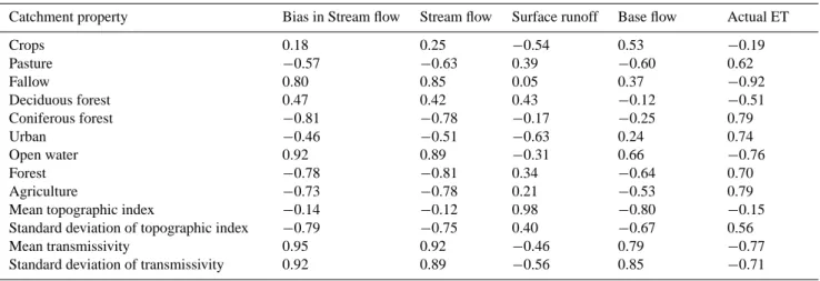
Table 8. Correlation coefficients (Pearson) between input data (transmissivity, topographic index, land use) and model results (water

bal-ances, biases) for the entire Dill catchment; forest = deciduous + coniferous forest; agriculture = crops + pasture.

Catchment property Bias in Stream flow Stream flow Surface runoff Base flow Actual ET

Crops 0.18 0.25 −0.54 0.53 −0.19 Pasture −0.57 −0.63 0.39 −0.60 0.62 Fallow 0.80 0.85 0.05 0.37 −0.92 Deciduous forest 0.47 0.42 0.43 −0.12 −0.51 Coniferous forest −0.81 −0.78 −0.17 −0.25 0.79 Urban −0.46 −0.51 −0.63 0.24 0.74 Open water 0.92 0.89 −0.31 0.66 −0.76 Forest −0.78 −0.81 0.34 −0.64 0.70 Agriculture −0.73 −0.78 0.21 −0.53 0.79

Mean topographic index −0.14 −0.12 0.98 −0.80 −0.15

Standard deviation of topographic index −0.79 −0.75 0.40 −0.67 0.56

Mean transmissivity 0.95 0.92 −0.46 0.79 −0.77

Standard deviation of transmissivity 0.92 0.89 −0.56 0.85 −0.71

is – as nonlinear and multivariate relationships hardly can be analysed for the huge number of computational units – sim-ply trying to quantify “linear” contributions of changes in input data sets to the sensitivity of the whole system. This

information later can be used for an analysis of model sensi-tivity with respect to data aggregation effects.

All spatial input data sets change significantly in statis-tics during aggregation. Increasing the grid size leads to a

(13)

(a) 6 6.5 7 7.5 8 8.5 9 9.5 10 10.5 11 10 100 1000 10000 grid size [m] m e a n t o p o g ra p h ic i n d e x Up.Dill Dietzhölze Aar Dill (b) 0.3 0.5 0.7 0.9 1.1 1.3 1.5 10 100 1000 10000 grid size [m] s ta n d a rd d e v ia ti o n o f to p o g ra p h ic i n d e x Up.Dill Dietzhölze Aar Dill

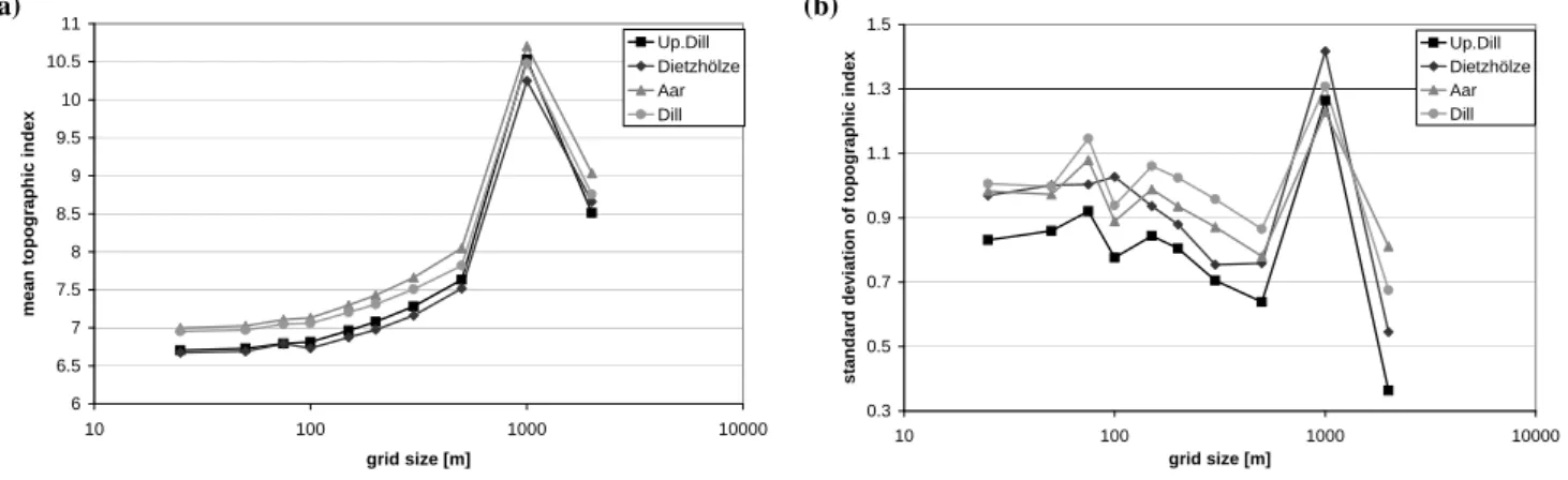
Fig. 8. Grid size dependent statistics of topographic catchment properties of the Dill catchment: mean value (a) and standard deviation (b)

of topographic index. (a) 0 2 4 6 8 10 12 10 100 1000 10000 grid size [m] m e a n t ra n s m is s iv it y

mean Up. Dill mean Dietzhölze mean Aar mean Dill (b) 0 10 20 30 40 50 60 10 100 1000 10000 grid size [m] s td a n d a rd d e v ia ti o n o f tr a n s m is s iv it y std.dev. Up.Dill std.dev. Dietzhölze std.dev. Aar std.dev. Dill

Fig. 9. Grid size dependent statistics of soil hydrological catchment properties of the Dill catchment: mean value (a) and standard deviation (b) of transmissivity.

smoothed surface of elevation and therefore to an increased mean topographic index (as cell size increases and slope in average decreases) and a decreasing standard deviation of the topographic index (Fig. 8). For single aggregation levels extreme values occur (e.g. 1000 m level for topographic in-dex) while the tendency is the same for all investigated catch-ments.

The transmissivity of the soils in general is barely affected by aggregation in a systematic way. Single extreme values occurring (Fig. 9) do not show a homogenous tendency for the different catchments. The behaviour strongly depends on local soil hydraulic conditions and soil depths.

The effect of aggregation on the land use fractions is exem-plarily shown for the entire Dill basin by Fig. 10. It becomes clear that the aggregation has no major effect up to a cell size of 500 m. Only at the 100 m level significant deviations for pasture and fallow land occur which was found to have an influence on the simulated water flows and model efficien-cies (Figs. 5, 6). For grid sizes lager than 500 m significant

changes in land use fractions can be observed for almost all land use classes. This is due to the fact that large areas grow at the expense of small areas, and grid sizes become larger than the average size of a homogenous area is. The effect of aggregation on land use fractions in the Dill catchment is comparable to the effects in the subcatchments which are summarised in Fig. 11.

To examine the contribution of the different data sources to the grid size dependent effects, a correlation analysis be-tween water balance components and catchment properties

was carried out. The correlation coefficients for the

en-tire Dill basin are summarised in Table 8. From the struc-ture of the simulation results it would first have been ex-pected that land use has a major influence on the simula-tions. This can be approved by the data. Forest areas are positively correlated to evapotranspiration and negative to stream flow production, while fallow areas and agricultural crops are correlated vice versa. Nevertheless one has to be careful because also spurious correlations appear in the data

(14)

(e.g. contrary correlation coefficients of coniferous and de-ciduous forest), and coherences between data and simulation results of course cannot be explained by linear correlations only. Nevertheless, water balance terms also show a clear dependence on soil and topographic characteristics. Surface runoff and base flow are highly correlated to the topographic index (surface runoff in a positive, base flow in a negative way), and transmissivity is correlated with base flow (pos-itively) and evapotranspiration (negatively) as well as sur-face runoff (negatively). To reduce spurious correlations the land use classes “forest” and “agriculture” were built from deciduous and coniferous forest as well as from crops and pasture. Analysing the correlation coefficients of these two merged land use classes several times the correlation coeffi-cient increases for the merged land use class which can be interpreted as increased significance of correlation and elim-ination of spurious correlation.

Simulation results are related to all spatial data sets, and evaluation of the effect of data aggregation therefore has to consider all data sources. Nevertheless it is worth to mention that predominantly the correlation between catchment prop-erties (e.g. topographic index, transmissivity, land use) and simulated water flows varies from catchment to catchment, in particular at the small scale. Partly this could be expected due to different physiographic characteristics of the subbasins (varying forest cover in the subbasins, different soil prop-erties), but partly the differences cannot be explained by the input data only and result from spurious correlations. One example for spurious correlations is the following: different signs were identified for the correlation between stream flow and deciduous forest (0.42) and coniferous forest (−0.78), respectively, while both classes together show a correlation coefficient of −0.81 which is below the value for coniferous forest. Additionally a correlation analysis between catch-ment average model parameters (e.g. plant parameters such as leaf area index, stomatal resistance) was performed. But also for catchment average model parameters the subcatch-ments showed different correlation, and the analysis could not reveal all reasons.

5 Conclusion: Limitations of model application This study indicates that an aggregation of input data for the calculation of regional water balances using TOPLATS type models does not lead to significant errors up to a grid size of 300 m. Between a grid size of 300 and 500 m a slightly to partly significant information loss leads to affected simu-lation results, while applying a grid size of 1 km and more causes significant errors in the computed water balance. If algorithms are integrated in a model taking into account sub-grid variability further investigations are required.

The results of this study indicate that a meaningful aggre-gation of data should in the first instance aim on preserving the areal fractions of land use classes, because land use is the

0 5 10 15 20 25 30 35 10 100 1000 10000 grid size [m] L a n d u s e D il l [% ] _agriculture pasture fallow dec. forest con. forest urban water

Fig. 10. Grid size dependent fractions of land use classes of the Dill

catchment.

most important information for this kind of SVAT schemes which are dominated by vertical processes such as evapo-transpiration. Nevertheless also the statistics of soil physical properties and topography should not be neglected. Aiming on total stream flow often masks effects of changes in fast and slow runoff components which may counterbalance their relative effects as shown above. Similarly, both the aggrega-tion procedure of input data itself and the model applicaaggrega-tion at decreasing spatial resolution (=increasing grid size) may cause changes in the simulation results, while in total both effects counterbalance to constant simulation results.

As the dependency of simulated water fluxes on grid size shows the same systematics for all investigated different sub-catchments and land use scenarios, the findings are transfer-able to other mesoscale catchments in humid and temper-ate environments. Within the investigtemper-ated range of

phys-iographic characteristics (e.g. 60–700 km2 catchment size,

700–1100 mm annual rainfall, 150–700 m elevation above sea level, 35–55% forest, 25–55% agriculture) the results are transferable to other catchments. The transferability to other model types is limited in so far, as TOPLATS focuses on ver-tical processes, and land use information is much more dom-inant than the influence of neighbouring grid cells. Other models are expected to show different sensitivities to aggre-gating input data, if neighbourhood relations and therefore lateral fluxes are considered in an explicit way. Therefore, the results need to be verified for models rather focusing on lateral processes which should be more sensitive to a smooth-ing of the topography.

Concluding, this investigation shows that high quality sim-ulation results require high quality input data but not always highly resolved data. The calculated water balances and sta-tistical quality measures do not get significantly worse up to spatial data resolutions which should be available in almost all developed and also in many developing countries. There-fore the focus while setting up data bases should be set to improve data quality first and then to optimise data resolu-tion secondly.

(15)

(a) 0 5 10 15 20 25 30 35 40 45 50 10 100 1000 10000 grid size [m] L a n d u s e u p p e r D il l [% ] agriculture pasture fallow dec. forest con. forest urban water (b) 0 5 10 15 20 25 30 35 40 45 50 10 100 1000 10000 grid size [m] L a n d u s e D ie tz h ö lz e [ % ] agriculture pasture fallow dec. forest con. forest urban water (c) 0 5 10 15 20 25 30 35 10 100 1000 10000 grid size [m] L a n d u s e A a r [% ] agriculture pasture fallow dec. forest con. forest urban water

Fig. 11. Grid size dependent fractions of land use classes of the upper Dill (a), the Dietzh¨olze (b), and the Aar catchment (c).

Acknowledgements. The author thanks the SFB 299 of the Uni-versity of Gießen for providing the data set in the framework of the LUCHEM initiative (special thanks to the organisers L. Breuer and S. Huisman) and the authors of the TOPLATS model (E. Wood and W. Crow in particular) for providing the model code and some support.

Edited by: S. Uhlenbrook

References

Andreassian, V., Perrin, C., Usart-Sanchez, I., and Lavabre, J.: Im-pact of imperfect rainfall knowledge on the efficiency and the pa-rameters of watershed models, J. Hydrol., 250, 206–223, 2001. Beven, K.: Linking parameters across scales: subgrid

parameteriza-tions and scale dependent hydrological models, in: Scale issues in hydrological modelling, edited by: Kalma, J. D. and Siva-palan, M., Advances in hydrological processes, Wiley, 263–281, 1995.

Beven, K. J., Lamb, R., Quinn, P. F., Romanowicz, R., and Freer, J.: TOPMODEL, in: Computer Models of Watershed Hydrology, edited by: Singh, V. P., Water Resources Publications, 627–668, 1995.

Booij, M. J.: Impact of climate change on river flooding assessed with different spatial model resolutions, J. Hydrol., 303, 176–

198, 2005.

Bormann, H., Faß, T., Junge, B., Diekkr¨uger, B., Reichert, B., and Skowronek, A.: From local hydrological process analysis to re-gional hydrological model application in Benin: concept, results and perspectives, Phys. Chem. Earth, 30(6–7), 347–356, 2005. Bormann, H. and Diekkr¨uger, B.: Possibilities and limitations of

regional hydrological models applied within an environmental change study in Benin (West Africa), Phys. Chem. Earth, 28(33– 36), 1323–1332, 2003.

Bormann, H., Diekkr¨uger, B., and Renschler, C.: Regionalization concept for hydrological modelling on different scales using a physically based model: results and evaluation, Phys. Chem. Earth B, 24(7), 799–804, 1999.

Breuer, L., Eckhardt, K., and Frede, H.-G.: Plant parameter values for models in temperate climates, Ecol. Model., 169, 237–293, 2003.

Brooks, R. H. and Corey, A. T.: Hydraulic properties of porous me-dia, in: Hydrology Paper, 3, 22–27, Colorado State University, Fort Collins, 1964.

Bruneau, P., Gascuel-Odoux, C., Robin, P., Merot, P., and Beven, K.: Sensitivity to space and time resolution of a hydrological model using digital elevation data, Hydrol. Processes, 9, 69–81, 1995.

Chen, E. and Mackay, D. S.: Effects of distribution-based parameter aggregation on spatially distributed agricultural nonpoint source pollution model, J. Hydrol., 295, 211–224, 2004.

(16)

Crow, W. T. and Wood, E. F.: The value of coarse-scale soil mois-ture observations for surface energy balance modeling, J. Hy-drometeorol., 3, 467–482, 2002.

Crow, W. T., Ryu, D., and Famiglietti, J. S.: Upscaling of field-scale soil moisture measurements using distributed land surface modeling, Adv. Water Resour., 28(1), 1–5, 2005.

Endreny, T. A., Wood, E. F., and Lettenmaier, D. P.: Satellite-derived elevation model accuracy: hydrological modeling re-quirements, Hydrol. Processes, 14(2), 177–194, 2000.

EU-WFD: EU Water Framework Directive 2000/60/EC of the European Parliament and Council, http://europa.eu.int/comm/ environment/water/water-framework/index en.html, date of ac-cess: 1 February 2006, 2000.

Famiglietti, J. S. and Wood, E. F.: Multiscale modelling of spatially variable water and energy balance processes, Water Resour. Res., 30(11), 3061–3078, 1994a.

Famiglietti, J. S. and Wood, E. F.: Application of multiscale water and energy balance models on the tallgrass prairie, Water Resour. Res., 30(11), 3079–3093, 1994b.

Farajalla, N. and Vieux, B.: Capturing the essential variability in distributed hydrological modeling: infiltration parameters, Hy-drol. Processes, 9, 55–68, 1995.

Fohrer, N., M¨oller, D., and Steiner, N.: An interdisciplinary mod-elling approach to evaluate the effects of land use change, Phys. Chem. Earth, 27, 655–662, 2002.

Gardner, W. R.: Some steady-state solutions of the unsaturated moisture flow equation with application to evaporation from a water table, Soil Sci., 85, 228–239, 1958.

Giertz, S.: Analyse der hydrologischen Prozesse in den sub-humiden Tropen Westafrikas unter besonderer Berücksichtigung der Landnutzung des Aguima-Einzugsgebietes in Benin, Disser-tation, Math.-Nat.-Fakultät der Universität Bonn (in German), Gemany, 2004.

HLBG: Hessische Verwaltung für Bodenmanagement und Geoin-formation, Digitales Geländemodell DGM25, available at: http: //www.hkvv.hessen.de/, (date of access: 1 February 2006), 2000. HLUG: Hessisches Landesamt für Umwelt und Geologie, Digital

soil map 1:50 000, 1998.

HLUG: Hessisches Landesamt f¨ur Umwelt und Geologie, Stream gauges in the Lahn basin, http://www.hlug.de/medien/wasser/ pegel/pg lahn.htm, (date of access: 1 February 2006), 2005. Kuo, W.-L., Steenhuis, T. S., McCulloch, C. E., Mohler, C. L.,

We-instein, D. A., DeGloria, S. D., and Swaney, D. P.: Effect of grid size on runoff and soil moisture for a variable-source-area hydrology model, Water Resour. Res., 35(11), 3419–3428, 1999. Lahmer, W., Pf¨utzner, B., and Becker, A.: Data-related Uncertain-ties in Meso- and Macroscale Hydrological Modelling, in: Ac-curacy 2000, edited by: Heuvelink, G. B. M. and Lemmens, M. J. P. M., Proceedings of the 4th international symposium on spa-tial accuracy assessment in natural resources and environmental sciences, Amsterdam, 389–396, 2000.

Milly, P. C. D.: An event based simulation model of moisture and energy fluxes at a bare soil surface, Water Resour. Res., 22, 1680–1692, 1986.

Monteith, J. L.: Evaporation and environment, in: Sympos. The state and movement of water in living organism, edited by: Fogy, G. T., Cambridge (Univ Press), 205–234, 1965.

Moore, I. D., Lewis, A., and Gallant, J. C.: Terrain attributes: Esti-mation methods and scale effects, in: Modelling change in

envi-ronmental systems, edited by: Jakeman, A. J., Beck, M. B., and McAleer, M., Wiley, New York, 189–214, 1993.

Nash, J. E. and Sutcliffe, J. V.: River flow forecasting through con-ceptual models, part I – a discussion of principles, J. Hydrol., 10, 272–290, 1970.

Omer, R. C., Nelson, E. J., and Zundel, A. K.: Impact of varied data resolution on hydraulic modelling and floodplain delineation, J. Am. Water Resour. As., 39(2), 467–475, 2003.

Pauwels, V. R. N., Hoeben, R., Verhoest, N. E. C., De Troch, F. P., and Troch, P. A.: Improvement of TOPLATS-based discharge predictions through assimilation of ERS-based remotely sensed soil moisture values, Hydrol. Process., 16(5), 995–1013, 2002. Pauwels, V. R. N. and Wood, E. F.: A soil-vegetation-atmosphere

transfer scheme for the modeling of water and energy balance processes in high latitudes. 1. Model improvements, J. Geophys. Res., 104(D22), 27 811–27 822, 1999a.

Pauwels, V. R. N. and Wood, E. F.: A soil-vegetation-atmosphere transfer scheme for the modelling of water and energy balance processes in high latitudes. 2. Application and validation, J. Geo-phys. Res., 104(D22), 27 823–27 840, 1999b.

Peters-Lidard, C. D., Zion, M. S., and Wood, E. F.: A soil-vegetation-atmosphere transfer scheme for modeling spatially variable water and energy balance processes, J. Geophys. Res., 102(D4), 4303–4324, 1997.

Quinn, P., Beven, K., Chevallier, P., and Planchon, O.: The predic-tion of hillslope flow paths for distributed hydrological modelling using digital terrain models, Hydrol. Processes, 5, 59–79, 1991. Rawls, W. J. and Brakensiek, D. L.: Prediction of soil water

prop-erties for hydrological modeling, in: Proceedings of the sympo-sium watershed management in the eighties, edited by: Jones, E. and Ward, T. J., Denver, 293–299, 1985.

Seuffert, G., Gross, P., and Simmer, C.: The Influence of Hydro-logic Modeling on the Predicted Local Weather: Two-Way Cou-pling of a Mesoscale Weather Prediction Model and a Land Sur-face Hydrologic Model, J. Hydrometeorol., 3(5), 505–523, 2002. Sivapalan, M., Takeuchi, K., Franks, S. W., Gupta, V. K., Karam-biri, H., Lakshmi, V. Liang, X., McDonnell, J. J., Mendiondo, E. M., O’Connell, P. E., Oki, T., Pomeroy, J. W., Schertzer, D., Uh-lenbrook, S., and Zehe, E.: IAHS Decade on Predictions in Un-gauged Basins (PUB), 2003–2012: Shaping an exciting future for the hydrological sciences, Hydrol. Sci. J., 48, 6, 857–880, 2003.

Sivapalan, M., Beven, K., and Wood, E. F.: On hydrologic similar-ity. 2. A scaled model of storm turnoff production, Water Resour. Res., 23, 2266–2278, 1987.

Skøien, J. O. and Bl¨oschl, G.: Characteristic space scales and timescales in hydrology, Water Resour. Res., 39(10), 1304, doi:10.1029/2002WR001736, 2003.

Thieken, A., L¨ucke, A., Diekkr¨uger, B., and Richter, O.: Scaling input data by GIS for hydrological modelling, Hydrol. Processes, 13, 611–630, 1999.

Wolock, D. M. and Price, C. V.: Effects of digital elevation model map scale and data resolution on a topography based watershed model, Water Resour. Res., 30(11), 3041–3052, 1994.

Zhang, W. and Montgomery, D. R.: Digital elevation model grid size, landscape representation, and hydrologic simulations, Wa-ter Resour. Res., 30, 1019–1028, 1994.