Algorithms and low power hardware for keyword spotting

Algorithms and Low Power Hardware for Keyword

Spotting

by

Miaorong Wang

B.S., Microelectronics, Shanghai Jiao Tong University (2016)

Submitted to the Department of Electrical Engineering and Computer

Science

in partial fulfillment of the requirements for the degree of

Master of Science in Electrical Engineering and Computer Science

at the

MASSACHUSETTS INSTITUTE OF TECHNOLOGY

June 2018

Massachusetts Institute of Technology 2018. All rights reserved.

Author .

.(

Signature redacted

C/

Department of Electrical Engineering and Computer Science

May 25, 2018

Certified by ...

Signature redacted

Anantha P. Chandrakasan

Vannevar Bush Professor of Electrical Engineering and Computer Science

Thesis Supervisor

Accepted by ...

Signature redacted

I

itIi

A. Kolodziejski

Professor of Electrical Engineering and Computer Science

Chair Department Committee on Graduate Students

MASSACHUSETTS INSTITUTE

Algorithms and Low Power Hardware for Keyword Spotting

by

Miaorong Wang

Submitted to the Department of Electrical Engineering and Computer Science on May 25, 2018, in partial fulfillment of the

requirements for the degree of

Master of Science in Electrical Engineering and Computer Science

Abstract

Keyword spotting (KWS) is widely used in mobile devices to provide hands-free inter-face. It continuously listens to all sound signals, detects specific keywords and triggers the downstream system. The key design target of a KWS system is to achieve high classification accuracy of specified keywords and have low power consumption while doing real-time processing of speech data. The algorithm based on convolutional neu-ral network (CNN) delivers high accuracy with small model size that can be stored in on-chip memory. However, the state-of-the-art NN accelerators either target at com-plex tasks using large CNN models, e.g. AlexNet, or support limited neural network

(NN) architectures which delivers lower classification accuracy for KWS. This thesis

takes an algorithm-and-hardware co-design approach to implement a low power NN accelerator for the KWS system that is able to process CNN with flexible structures.

On the algorithm side, we propose a weight tuning method that tweaks the bits of weights to lower the switching activity in the weight network-on-chip (NoC) and multipliers. The algorithm takes in 2's complement 8-bit original weights and out-puts sign-magnitude 8-bit tuned weights. In our experiment, 60.96% reduction in the toggle count of weights is achieved with 0.75% loss in accuracy. On the hardware side, we implement a processing element (PE) to efficiently process the tuned weights. It takes in sign-magnitude weights and input activations, and multiplies them by an unsigned multiplier. An XOR gate is used to generate the sign bit of the product. The sign-magnitude product is converted back to 2's complement representation and accumulated using an adder-and-subtractor. The sign bit of the product is used as a carry bit to do the conversion. Comparing to the PE that processes original 2's complement weights, around 35% power reduction is observed. In the end, this thesis presents a CNN accelerator that consumes 1.2 mW when doing real-time process-ing of speech data with an accuracy of around 87.3% on Google speech command dataset [34].

Thesis Supervisor: Anantha P. Chandrakasan

Acknowledgments

This thesis would not have been possible without the help of a large group of people. First of all, I would like to thank my thesis supervisor, Professor Anantha Chan-drakasan. Thank you for letting me into your group, offering me the opportunity to work on this interesting project and providing research directions along the way. Your encouragement, support and guidance are invaluable to me.

Next, I would like to thank Michael Price for his great help in this project. Al-though he has graduated before I joined this group, he is always willing to provide guidance and answer technical questions either in person or through emails.

I also owe a debt of gratitude to several of my colleagues. I am thankful to

Utsav Banerjee, Priyanka Raina and Skanda Koppula for their technical assistance. And I would like to thank Chiraag Juvekar and Avishek Biswas for their helpful discussion and feedback on my research directions. Special thanks to Avishek Biswas for providing feedback on my thesis.

Besides, I want to thank all the Ananthagroup members. It has been a wonderful experience to work with those talented people from all over the world. I learned a lot from them.

I would also thank Cheng Wang for helpful discussions when I encountered

prob-lems, and great collaboration we had in the course project.

I would like to thank my sponsors for their generous supports. My first year is supported by Irwin Mark Jacobs and Joan Klein Jacobs Presidential Fellowship. And the second year is sponsored by Foxconn Technology Group. Thanks for making this project possible.

Aside from this project, I would like to thank the publicity co-chairs of Sydney-Pacific, Grace Liu, Chia-Jung Chang, Demi Fang and Li-Wen Wang, for their great collaboration in finishing the publicity work especially when I was busy.

And finally, I would like to express my gratitude to my parents for loving and supporting me along the way. They always encourage me to chase my dreams and have great confidence in me. That makes the person I am today.

Contents

1 Introduction

11

1.1 Background and Motivation . . . . 11

1.1.1 System Design Targets . . . . 11

1.1.2 KWS Algorithms . . . . 12

1.1.3 Hardware Design . . . . 14

1.1.4 Algorithm and Hardware Co-design . . . . 15

1.1.5 Research Focus . . . . 17

1.2 System Overview . . . . 18

1.3 Thesis Overview and Contributions . . . . 19

2 Bit Tuning Algorithm 21 2.1 O verview . . . . 21

2.2 Tensor Decomposition and Retraining . . . . 22

2.3 Sign-Magnitude Representation . . . . 24

2.4 Weight Scaling . . . . 27

2.5 Bit Perturbation . . . . 31

2.6 Fine Tuning . . . . 34

3 Dataflow Analysis 39 3.1 Convolutional Neural Network (CNN) . . . . 39

3.2 Convolution Loop Nest . . . . 41

3.3 Comparison of Different Dataflows . . . . 42

3.3.2 Output Stationary (OS) . . . . 51 3.3.3 Row Stationary (RS) . . . . 55 3.3.4 No Local Reuse (NLR) . . . . 55 3.4 R esults . . . . 57 4 Hardware Design 59 4.1 O verview . . . . 59

4.2 Processing Element (PE) Structure . . . . 60

4.3 Mapping Filters to PE Array . . . . 62

4.4 Network-on-Chip . . . . 63

4.5 Synthesis and Simulation Results . . . . 64

4.5.1 P E . . . . 64

4.5.2 NN Accelerator . . . . 65

5 Conclusions and Future Work 69 5.1 Summary . . . . 69

5.2 Future Work . . . . 70

List of Figures

1-1 Top level diagram of a keyword spotting system. . . . . 13

1-2 A comparison of different NNs on accuracy, the number of operations (ops) and memory size under the constraints of 80kB memory and 6MOps [37 on Google speech command dataset

[34].

The memory size is depicted by the size of the bubble. . . . . 14

1-3 Research focus of designing a NN accelerator for highly accurate, real-time and low-power KWS system. . . . . 18

1-4 An illustration of the hardware and software co-design approach. . . . 20

2-1 An illustration of tensor decomposition on CONV layers. . . . . 23

2-2 The influence of weight bitwidth on accuracy. . . . . 26

2-3 The histogram of weights in the first layer of CNN-1. . . . . 27

2-4 ReLU function. . . . . 29

2-5 The flowchart of fine tuning. . . . . 36

3-1 An illustration of calculation in a CONV/FC layer. . . . . 40

3-2 Loop nest of a CONV layer. . . . . 42

3-3 A simple case of WS. . . . . 44

3-4 The illustration of WS-1. A register file with the size of 1 x C for input activations is drawn in PE for illustration. Only one register is needed in actual implementation. . . . . 46

3-5 Loop nest of W S-1. . . . . 46

3-6 The illustration of WS-2. A register file with the size of 1 x R x S for input activations is drawn in PE for illustration. Only one register is needed in actual implementation. . . . . 48

3-7 Loop nest of W S-2. . . . . 48

3-8 The illustration of WS-3. A register file with the size of 1 x R x S for input activations is drawn in PE for illustration. Only one register is needed in actual implementation. . . . . 49

3-9 Loop nest of W S-3. . . . . 49

3-10 The illustration of WS-4. A register file with the size of 1 x C for input activations is drawn in PE for illustration. Only one register is needed in actual implementation. . . . . 50

3-11 Loop nest of W S-4. . . . . 51

3-12 The illustration of OS-Chn. . . . . 53

3-14 The illustration of OS-EF. Register files with the size of 1 x R x S for

input activations and weights are drawn in PE for illustration. Only

one register is needed for both data in actual implementation. .... 54

3-15 Loop nest of OS-EF. . . . . 54

3-16 The illustration of RS. . . . . 56

3-17 Loop nest of RS. . . . . 56

3-18 The comparison of different dataflows on CNN-1-decomp. . . . . 58

4-1 System architecture of the NN accelerator for KWS. . . . . 60

4-2 The PE structure. . . . . 61

4-3 An illustration of mapping a filter with M = 21 and C = 10 to the PE array following the WS-1 dataflow. . . . . 63

4-4 NoC for weights and the micro-architecture of the unicast/multicast controller [7]. . . . . 64

4-5 The power break down of PE, and PEb. . . . . 65

Chapter 1

Introduction

1.1

Background and Motivation

1.1.1

System Design Targets

Keyword spotting (KWS) is widely used in mobile devices or Internet-of-Things (IoT)

applications to provide hands-free interface. It detects specific keywords and triggers

the corresponding downstream system. For example, Apple's conversational assistant

named Siri listens to 'Hey Siri' to initiate voice input for speech recognition. To

enable efficient application, three design targets should be met for a KWS system, including low latency, low power consumption and high accuracy.

Low Latency

The KWS system needs to process real-time speech waveform and generates trigger

signals as soon as the user utters the specified keywords. Typically a frame of speech

features is extracted and needed to be processed every 10 ms to 20 ms for KWS. This

Low Power Consumption

The KWS system is always-on and serves as a trigger to some downstream systems.

Since the battery life is important to mobile/IoT applications, power consumption of the KWS system should be minimized.

High Accuracy

When the KWS system detects specified keywords, it powers up the downstream system. The downstream system is usually much larger and consumes more power than the KWS system. One example of the downstream system is a speech recognizer. The work [26] consumes 1.8-7.8 mW on-chip power and the power hungry DRAM access is needed for typical speech recognition tasks, which leads to large overall system power. A false alarm generated by the KWS system will waste a large amount of energy on powering up the downstream system. Besides, large false rejection rate leads to frequent miss of keywords and thus has a negative impact on user experience. Given those two aspects, achieving high accuracy in the KWS system is critical.

1.1.2

KWS Algorithms

State-of-the-art algorithms for KWS are based on neural networks (NNs). A diagram which illustrates a classification of the word 'yes' in the KWS system is shown in Fig. 1-1. It takes in sampled speech data as the inputs and outputs a 1-D vector to indicate which keyword is detected [4]. The system is composed of three stages. First, a front-end unit extracts acoustic features from speech waveforms. Second, a NN computes the posterior probability of each specified keyword, given the acoustic features at each time step. In the last stage, a posterior handling unit smooths the outputs of the NN within a given time window to filter out classification noise. It then outputs a 1-D vector indicating which keyword is detected in this window. The accuracy and power consumption of the whole system are mainly determined by the

NN block.

Neural Network

--

C

P('yes'IA)

Sampled waveform

C

P('no'IA)

of the word 'yes'

Feature Posterior 0 Extraction - Handling .z -- P(<sil>IA) C0 -w

C)

P(OOVIA) A: acoustic features <sil>: silence

OOV: out-of-vocabulary word

Figure 1-1: Top level diagram of a keyword spotting system.

A large variety of NNs have been employed in the KWS system. Multi-layer

perceptron (MLP) is first implemented in the KWS system shown in Fig. 1-1 [4]. Then a paper, co-authored by one of the researchers in the previous work, shows that convolutional neural network (CNN) outperforms MLP in the KWS task [29]. Later on, NNs, such as recurrent neural network (RNN) [31], convolutional recurrent neural network (CRNN) [1], etc. were explored. Different works use different datasets to train the NNs and the criterion to choose the architectures varies. To give a direct comparison of various NNs, Y. Zhang trains different NNs on the same speech command dataset [34]. The architecture for each type of NN is chosen to have the best performance under certain memory and operation constraints. Under the constraint of 80kB memory and 6MOps, Fig. 1-2 illustrates the comparison of different types of NNs. As shown, MLP has much larger memory size over ops ratio compared to other NNs, and delivers relatively low accuracy.

To summarize, different NN architectures have different computation and memory requirements, and provide varied accuracies. MLP requires less computation, but has lower accuracy compared to other types of NNs for KWS tasks. Thus for a system requiring high accuracy, a NN accelerator designed only for MLP processing may not

fit.

98 96 38.6KB 94-92 *MLP

9CNN

901-SLSTM 88 - GRU 86 _CRNN --80.OKB DS-CNN 84 82 -1 0 1 2 3 4 5 6 7 8 MOps

Figure 1-2: A comparison of different NNs on accuracy, the number of operations (ops) and memory size under the constraints of 80kB memory and 6MOps [37] on

Google speech command dataset [34]. The memory size is depicted by the size of the

bubble.

1.1.3

Hardware Design

This work focuses on a chip implementation of a full KWS system including the

feature extraction unit, the NN accelerator and the posterior handling unit.

Recent research has presented many convolutional neural network (CNN) acceler-ators for high-complexity tasks using large networks requiring off-chip memory access

as shown in Table 1.1. Dataflow and architecture of the designs are optimized to

lower the off-chip memory access, since it consumes around 100x more energy than

on-chip memory access and computation [5].

Several NN accelerators has been designed for moderate-complexity tasks with

Table 1.1: Examples of CNN accelerators for high-complexity tasks.

Reference Paper Supported Layers Off-chip Memory Access Power (mW)

Chen, ISSCC 17 [6] CONV off-chip DRAM 278

Lee, ISSCC 18 [22] FC, CONV, RNN off-chip DRAM 3.2 - 297t

Ueyoshi, ISSCC 18 [33] FC, CONV, RNN 3D SRAM3300

using inductive-coupling

t Power for off-chip memory access is not included.

are designed for MLP, which has lower accuracy for KWS tasks, compared to other

types of NNs. [3] can process convolutional layers, but only a fixed shape of filter is

supported and the network should be binarized. This results in the loss of flexibility.

And binary neural network (BNN) delivers lower accuracy compared to the floating point counterparts, e.g. 29.8% accuracy loss on ImageNet [9] dataset [32].

Table 1.2: Examples of NN accelerators for moderate-complexity tasks.

Reference Paper Whatmough, ISSCC 17 [35]

Bang, ISSCC 17 [2]

Shah, SiPS 15 [30]

Bankman, ISSCC 18 [3]

Supported Layers Off-chip Memory

FC none FC none FC none FCn binarized CONV Power (mW) 22.4 0.321 3.3 0.889

1.1.4

Algorithm and Hardware Co-design

Although NNs deliver state-of-the-art performance in many applications, they are power hungry and thus, difficult to be implemented in IoT devices. To improve the energy efficiency, many algorithms are proposed to co-design the NN and its corre-sponding hardware accelerator. Those algorithms can be divided into two groups [32]:

. quantization

Quantization

Quantization

is to map floating-point parameters in NN to a smaller set of quantized values. It reduces the complexity of the computation units and lowers the amount

of storage since less bits are needed to represent the parameters. One popularly

used quantizer is the linear quantizer. It is simply the fixed-point representation of

numbers. Fixed point calculation units are used to process the NNs instead of the

floating-point counterparts. Next, log2 quantizer is also explored [21]. After mapping

data into the log2 domain, multiplication can be converted to shifting. But it increases

the complexity of addition. Addition can be done either in the linear domain with

additional domain conversion steps or in the log2 domain using an approximation

algorithm. Another type of non-linear quantizer uses a quantization function learned

from data. For example, data are clustered into groups using k-mean [14]. The mean

of each group is used to represent the group of data. Since the quantization function

is complicated, a look-up table and an index calculation unit to align weights and

activations are needed to perform calculation on hardware.

Extreme cases of quantization are the tenary weight network [23, 38] and the

binary weight network [8, 28]. The weights and/or activations in those networks are

quantized into only one to two bits. It significantly reduces the storage, but has

several drawbacks. If all layers of weights are quantized into one to two bits, the

classification accuracy drops greatly. The accuracy may be maintained by keeping

the first and the last layer of weights from this extreme way of quantization. However, it imposes a great challenge on the ASIC design to support both tenary/binary weight

layers and normal layers with relatively large bitwidth.

Model Compression

Model compression is to reduce the model size and the number of operations with an

Methods in the first category are pruning-based, which set low-magnitude weights and/or activations to zero. Related works can be found in [15], [36], etc. During hardware implementation, multiplication with zero is skipped to minimize the com-putation energy. And weights should be compressed to be zero-free before stored in the memories so that the memory power consumption can be lowered. Those require dedicated hardware to process the compressed data. Related works can be found in [13, 25], etc. For large NN with over 10M weights, weights cannot be fit in the on-chip SRAM. Thus off-chip memory access is needed, which takes up a large por-tion of the total power consumppor-tion. Using pruning-based method and dedicated hardware improves energy efficiency, because pruning greatly reduce the number of weights and/or activations, and thus reduces the number of off-chip memory accesses required. But for small NN that can be stored on chip, it is not clear whether using a more complex hardware architecture to handle pruned weights and/or activations provides higher energy efficiency.

The other category of methods does not leverage the zeros in weights and/or activations. It compacts the NN architecture. For example, tensor decomposition is applied to NN after training to approximate large weight tensors using a sequence of small tensors [17, 20]. It is reported to have similar compression rate and accuracy loss compared to the pruning based methods. On top of that, it eliminates the need for dedicated hardware architecture.

1.1.5

Research Focus

This thesis targets at the complete system implementation for KWS application, cov-ering the functions of feature extraction, NN processing and posterior handling. A

highly accurate, real-time and low-power KWS system imposes the need for a NN

ac-celerator that falls in the gap between existing designs, as shown in Fig. 1-3. And the existing algorithm and hardware co-design techniques focus on reducing the memory

footprint and the number of operations. The influence of bit flips in the hardware

on the energy consumption and how to utilize it have not analyzed. This thesis

fo-cuses on designing a NN accelerator using a novel algorithm-and-hardware co-design

technique. The NN accelerator supports CNN in order to deliver high accuracy for

keyword detection. It is optimized for medium size NNs with less than 80kB

param-eter size and around 5MOps to achieve low power consumption under the latency

constraint for real-time processing.

2 2

z

This work Table 1.1 &

Z

similar works

Table

1.2

&

2F similar works

Power

Figure 1-3: Research focus of designing a NN accelerator for highly accurate, real-time and low-power KWS system.

1.2

System Overview

We take a hardware and software co-design approach to implement the accurate, low-power and real-time KWS system, as illustrated in Fig. 1-4.

The raw model mainly determines the accuracy of the KWS system. Designing

the hardware architecture to support existing CNN architectures guarantees the high

accuracy of the system.

the memory size, tensor decomposition [17] is applied and a compressed model is

generated with little loss of accuracy. The dataflow of the NN accelerator mainly de-termines the number of memory accesses needed to process a NN. Different dataflows

are analyzed and a weight stationary dataflow is found to work best for the NNs for

our KWS system.

We also investigated into reducing the power consumption from the other parts

of the NN accelerator. Dynamic power of a CMOS gate is determined by load

capac-itance (CL), operation frequency (f), switching activity (ao_>1), and supply voltage

(Vdd), as shown in the following equation.

Pdyn =

aooCLVdf

(1.1)

We tried to minimize each component. First, tensor decomposition reduces the

amount of computation required in a NN. Thus lower clock frequency and supply

voltage can be used to process the NN. Second, a spatial hardware architecture is

designed to optimize the clock frequency and effective load capacitance of the system,

and to meet the real-time requirement. Finally, a bit tuning algorithm is proposed

to lower the switching activity on the weight bus and the multipliers with marginal

loss of accuracy. It also provides the opportunity of using a custom memory pro-posed in [11], which is reported to reduce around 50% of the read access energy, given certain data statistics.

1.3

Thesis Overview and Contributions

This thesis takes a algorithm-and-hardware co-design approach to optimize the energy efficiency of the KWS system achieving high accuracy and real-time processing.

Chapter 2 proposes an algorithm to tune the bits of fixed-point weights, which

software

dateset

quantize &

raw compress computa tun

low-train

meswitching-e N actit model

architecture _--

reduce dynamic reduce memory size & the power influence amount of computation

dataflow Rm) meow r y

NN accelerator

optimize

architecture armlutatel n

hardware

Figure 1-4: An illustration of the hardware and software co-design approach.

discussed in detail, along with training and testing results to show its influence on

NN classification accuracy.

Chapter 3 provides a comprehensive analysis of the dataflows for the NN

accel-erator. The number of memory accesses using weight stationary (WS), output

sta-tionary (OS) and row stasta-tionary (RS) dataflow are analyzed under certain hardware

constraints. Based on the analysis and comparison, WS dataflow is used for our NN

accelerator for KWS.

Chapter 4 presents a NN accelerator supporting weight stationary dataflow.

Hard-ware architectures and micro-architectures are illustrated. Processing elements (PEs) running the original NN model and the model tuned by the algorithm proposed in Chapter 2 are compared. It proves the effectiveness of the proposed algorithm in

energy reduction. The simulation results of the whole NN accelerator are presented.

Chapter 5 summarizes the key contributions of the thesis and presents the future

Chapter 2

Bit Tuning Algorithm

2.1

Overview

The power consumption of a NN accelerator can be reduced by tuning the bit repre-sentation of weights. As shown in Eq. 1.1, dynamic power of a CMOS gate is linearly proportional to the switching activity ao_,. In a NN accelerator, weights are read from the buffer, delivered through network-on-chip (NoC) and then multiplied with input activations. The reading, delivery and processing sequence of weights are fixed

by the designer. The bit toggling between consecutive weights affects the switching

activity of weight buses and the multipliers. And for a memory that utilizes data statistics, e.g. [11], it also influences the switching activity of bit lines. Therefore min-imizing the bit toggle count of weights reduces the power consumption of multipliers, the weight NoC and even the SRAM.

We propose an algorithm that tunes the bits of weights to lower the amount of bit toggling with insignificant loss in accuracy. A CNN is tuned by the following steps.

1. Tensor decomposition and retraining

2. Fixed-point sign-magnitude representation

4. Bit perturbation

5. Fine tuning

This chapter will introduce each step and the experimental results will also be

pre-sented.

2.2

Tensor Decomposition and Retraining

Tensor decomposition is used to compressed the model size and the number of

cal-culations in the NN with little loss of accuracy after retraining [17, 20]. The reason

to include it as a step in our bit tuning algorithm for CNN is that, it magnifies the

influence of weights on the switching activity of the multiplier. This will be explained

in the following analysis.

We adopt the compression scheme proposed in [17]. The filter (W) with the

shape of M x C x R x S can be decomposed into three smaller filters using Tucker-2

decomposition. It can be written as follows:

R3 R₄ Wrs,c,m =

S S

Kr,,r3,r4

X

3 Xr 4 (2.1) r3=1 r4=1 R₂ R₄ Kr,r2,c,r4

Xs

2 (2.2) r2=1 r4=1

where R2, R3 and R4 are the rank of the mode-2, mode-3 and mode-4 matricization

of the tensor W respectively. K is the core tensor and X(2), X(3) and X(4) are factor matrices of sizes S x R2

, C

x R3 and M x R4 respectively. For most CONV layers, R

and S are relatively small. Thus Eq. 2.1 is used to decompose mode-3 and mode-4 that

are associated with the input and output channel dimensions. It is depicted in Fig. 2-1.

X(3) and X(4) are used as 1 x 1 convolution filters. The output activations generated by the lower part of the graph should be similar to the upper part. Activation functions,

such as ReLU, are only applied to the final outputs. Intermediate layers are just

linear transformation. For the first layer of the CNN for KWS, where

C =

1, Eq. 2.2

is used instead. Detailed explanantion of tensor decomposition and the tool chain

can be found in [17].

Tensor decomposition generates a compressed NN architecture and also provides

the values of every decomposed tensors. Because the reconstruction error of the weight

tensors, instead of the output activations, are minimized during tensor decomposition,

directly using the decomposed filters results in significant loss in accuracy (e.g. more

than 50% in AlexNet [17]). Therefore, retraining is needed. The decomposed filter

values are used as the starting point.

M

Input acivation w output activation

9 decompoettion

Input activation reuf

Figure 2-1: An illustration of tensor decomposition on CONV layers.

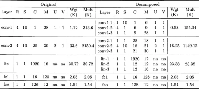
Table 2.1 shows the decomposition of a CNN trained for KWS on the Google

speech command dataset [34] in [37]. The decomposed models are trained using the

experimental setup in [37]. But batch normalization is not applied, because it is

cur-rently not supported in our NN accelerator. The classification accuracy evaluated on

the test set is reported. The original and decomposed NN will be referred to as

layers (conv1, conv2) and the linear-low-rank layer (lin) take up a large portion of

the total parameter size and the amount of computation, and thus are decomposed.

In our experiments, decomposing the first fully-connected layer (fcl) and the output

layer (fco) leads to great accuracy loss and thus they are kept unchanged. Although

the original network is designed to be small-footprint, tensor decomposition further

reduces the parameter size and the amount of computation.

We conducted experiments on other existing CNN architectures for KWS trained

on the Google speech command dataset [34]. Table 2.2 summaries the effect of tensor

decomposition on those CNN architectures. The architecture of CNN-2 is proposed

in [37]. CNN-3 refers to the fstride4 architecture in [1]. The decomposed versions

are referred to as CNN-2-decomp and CNN-3-decomp in the rest of this thesis. The

detailed structure can be found in Appendix A. As shown, tensor decomposition with

retraining has little effect on the accuracy for all different types of CNN for KWS.

Besides the reduction in the parameter size and the amount of computation, the

reason why we apply tensor decomposition before tuning the weights of CNN are as

follows. Most CNNs use ReLU as the activation function. In our experiments, a

large portion of output activations are set to be zero after ReLU. An efficient way to

process a large number of zero activations is to use data gating to skip the multiplier

and weight read inside the PE [7]. Thus it reduces the influence of weights on the

switching activity of the multiplier. Tensor decomposition generates several linear

layers that are not followed by activation functions, thus improves our control of the

switching activity of multipliers through bit tuning the weights.

2.3

Sign-Magnitude Representation

After we decomposed and retrained the CNN, we use linear quantizer to convert

Table 2.1: The original and decomposed architecture of CNN-1. The input layer of

CNN-1 has H = 10 and W = 49.

Original Decomposed

Layer R S C M U W ult Layer R S C M U V gt lult

U (K) (K) Lyr(K) (K) conv1-1 1 10 1 6 1 1 conv1 4 10 1 28 1 1 1.12 313.6 conv1-2 4 1 6 9 1 1 0.53 155.04 conv1-3 1 1 9 28 1 1 conv2-1 1 1 28 18 1 1 conv2 4 10 28 30 2 1 33.6 2150.4 conv2-2 4 10 18 21 2 1 16.25 1149.12 conv2-3 1 1 21 30 1 1 lin-1 1 1 1920 12 na na lin 1 1 1920 16 na na 30.72 30.72 lin-2 1 1 12 12 na na 23.38 23.38 lin-3 1 1 12 16 na na fel 1 1 16 128 na na 2.05 2.05 fcl 1 1 16 128 na na 2.05 2.05 fco

I1

1 128 12 na na 1.54 1.54j fco I1 1 128 12 na na 1.54 1.54 R, C, U,

S: Length of filter in time and frequency axis

M: Number of input and output channels V: Stride in time and frequency

Table 2.2: Comparison of accuracy, parameter size and before and after tensor decomposition and retraining.

the amount of computation

CNN Accuracy (%)

Orig. Decomp. Loss

CNN-1 89.78

88.54

1.24

CNN-2 90.94

90.65

0.29

CNN-3 81.90

81.20

0.70

t Compression rate

I Speed-up rate

Orig 69.0K

178.2Kb

949.4Kh Parameters Decomp. 43.7K 120.8K 88.4K Multiplications

CRt Orig Decomp. SRI

1.58x 2.5M 1.3M 1.92x

1.48x 8.6M 6.OM 1.43x

10.74x 5.6M 0.5M 11.2x

accelerator. It is proved by many works, e.g. [12, 37], that storing weights in 8-bit is enough for maintaining good accuracy. Fig. 2-2 shows our experimental results on the decomposed CNN models mentioned in Table 2.2. Bit width of 8 delivers almost the same performance as the floating point NN. Weights have both positive and negative values. In most cases, 2's complement representation is used to handle signed numbers, due to its simplicity in computation. Thus we use 8-bit fixed-point 2's complement weights as the baseline of our bit tuning algorithm.

Compared to 2's complement representation, sign-magnitude weights have much lower toggle count. Table 2.3 presents the total number of 0-to-1 toggle given the processing sequence of our NN accelerator. Around 30%-40% of reduction can be made by converting weights from 2's complement to sign-magnitude. The reason is

that weights of each layer roughly follows zero-mean Gaussian distribution as shown

in Fig. 2-3. The majority of them are close to zero. 2's complement representation

of two small numbers with opposite sign has large toggle count, because of the sign

bits. Sign-magnitude representation does not have this issue.

The cost of using sign-magnitude representation is that the adder needed for it is

more complex than the 2's complement adder. Two 2's complement numbers can be

added up using a signed adder. But for the sign-magnitude numbers, we need to first

check the sign to determine whether addition or subtraction is needed. Making use

of the fixed computation pattern of NN, we propose a mixed-representation

process-ing element (PE) that minimizes the hardware cost of usprocess-ing sign-magnitude weights.

Section 4.2 discusses it in detail.

100 -80 - """""""" "s

60

140 -- -CNN-1-decomp -4-CNN-2-decomp 20 -A-CNN-3-decomp ... CNN-1 floating-point ... CNN-2 floating-poin . ...CNN-3 floating-poin 0 2 4 6 8 10 12 14 16 bit width

Table 2.3: The 0- > 1 toggle count of 2's complement and sign-magnitude weights.

CNN

2's complement sign-magnitude reduction

CNN-1-decomp

79793

55623

30.3%

CNN-2-decomp

232752

125178

46.2%

CNN-3-decomp

172537

114717

33.5%

70- 60- 50-4.0

C

0

U 40 30 20 10 -0.3 -0.2 -0.1 0.0 0.1 0.2 0.3

weight

Figure 2-3: The histogram of weights in the first layer of CNN-1.

2.4

Weight Scaling

Weight scaling is to multiply the weights with a number k that is bigger than 0.5

and smaller than 2. The multiplication is done in floating-point and then the weights

are converted back to 8-bit fixed-point. Since 0.5

<

k

<

2, weight scaling does not

change the location of the decimal point.

0

If we assume that the precision of weight and calculation is unlimited, scaling

weight does not affect the accuracy of NNs that use ReLU as their activation function.

The output activation can be calculated as follows:

O[m][e][f

]

=

ReLU(B[m]

r=R-1 s=S-1 c=C-1

+ E E E I[c][Ue-

+ f][Vf + s]

x

W[m][c][r][s]),

r=0 8=0 c=0

(2.3)

0<m<M,0<e<E,0<f<F,

E =(H - R+U)/UF =(W - S+V)/V

where

0, I,

B and W stand for output activations, input activations, biases and

weights respectively. The explanation of indices are listed in Table 3.1. After weight

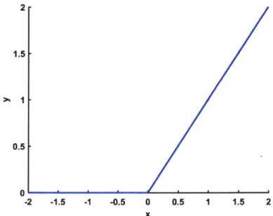
scaling, we have W' = kW and B' = kB. As shown in Fig. 2-4, ReLU(kx) =

kReLU(x). Thus we have the following equation:

0'[in]

[e] [f]

= ReLU(B[m]

r=R-1 s==S-1 c=C-1

+

E

E

5

I[c][Ue+ f][Vf + s]

x

W'[m][c][r][s]),

r=O S=0 c=0 = ReLU(kB[m] r=R-1 s=S-1 c=C-1

+ k E

E E I[c][Ue + f][Vf + s]

x

W[m][c][r][s])

r=0 s=0 c=0 =

_{k x}

_O[m][e][f]

(2.4)

Linear scaling of weights result in linear scaling of output activations. The outputs of the last layer are connected to softmax function, which is shown in Eq. 2.5.

-(z)m = Mez

n= Al

M =

1,

...

,

7M

where z is M-dimension output vector of the last layer. It can be proved that

o-(kz)m

= o-(z)m

_(2.6)

M = 1, ... ,M.

Thus linear scaling of weights does not affect the final output of a

NN.

2 1.5 0.5 0' -2 -1.5 -1 -0.5 0 0.5 1 1.5 2 x

Figure 2-4: ReLU function.

In reality, weights are stored in 8-bit. When we scale the weights in floating point

numbers and convert them back to fixed-point numbers, truncation of bit introduces

nonlinearity. Thus the effective scales of different 8-bit numbers may be different.

Table 2.4 shows an example. Original weights 0.15625 and 0.9921875 are multiplied

with 0.8, and the products are 0.125 and 0.79375 respectively. We have weights

stored in Q1.7 format. 0.125 can be directly represented in this format, while 0.79375

needs to be truncated. The Q1.7 fixed-point representation of 0.79375 has a decimal

value of 0.7890625, which results in an effective scale of around 0.795 instead of 0.800.

Although all the weights in one layer are multiplied with the same number in floating

point, the effective scales for fixed point numbers may be different. Thus weight

scaling can lead to some accuracy loss of the overall system.

Table 2.4: An example of weight scaling.

Original Wgt Scale Scaled Wgt Effective

Decimal

Fxpt

Decimal

Fxpt

Scale

0.15625 0.0010100 0.125 0.0010000 0.800 0.9921875 0.1111111 0.79375 0.1100101 0.795

Weight scaling is done following the Algorithm 1. We search for the scale that

results in the smallest toggle count in a given range. Since the average magnitude

of weights affects the average magnitude of activations at each layer, we need to

scale the activations to prevent them from overflow or underflow for the fixed-point

representation. After weights are tuned, we gather all the weight scale and determines

the activation scale using Algorithm 2. Activations at each layer is kept unchanged

or increased by a factor of 2 or 0.5. This can be done using a 1-bit shifter, which is

implemented by simple rewiring.

Input: Weights of one layer W, scale range [a, b] (a > 0.5, b < 2) and step s Output: Scaled weights Wbest, corresponding scale kbest

1 TC +- CountToggle (W); 2 minTC <- TC; 3

k

+-

a;

4

while k < b do

5

W' = k

x

W;

6 newTC <- CountToggle(W');

7 if newTC < minTC then

8 minTC <- newTC; 9 Wbest <- W' 10 kbest --

k;

11 end 12 k +- a+ s; 13 end

Input: Weight scale k, of this layer, weight scale k1+1 of next layer,

accumulated weight scale kacc from the first layer to previous layer

Output: Output activation scale tj of this layer, accumulated weight scale k' from the first layer to this layer

1 k'c <- kacc x ki;

2 ifk

' x k

_acc 1

+

1

<= 0.5 then ti <- 2;

3 else if k' x k1+1 >= 2 then t1 +- 0.5; 4 else tj <- 1;

Algorithm 2: Pseudo-code for deriving activation scale for each layer.

2.5

Bit Perturbation

Inspired by the power reducing technique proposed for FIR filter [16], we perturb the

bits of weights to further reduce the switching activity. Since we tweak the bits of weights, the weight values change after bit perturbation. Averaged relative error of

all data is used to represent the tuning error. Relative error is defined as

e =IVVol (2.7)

|vol

where v0 and v is the original value and the perturbed value respectively. Given the

maximum relative error emax the system can tolerate, bit perturbation of weights is

done in the following steps.

1. Flatten the 4-D weight tensor into a 1-D vector following the sequence that

weights are read, delivered and calculated in the NN accelerator

2. Split the large 1-D vector into smaller vectors with the length of L

3. Perturb every small 1-D vector using Algorithm 3, given the maximum relative

error emax the system can tolerate

4. Concatenate the perturbed vector and reshape them to the 4-D weight tensor

L and emax are the parameters the designer can play with. They both affect the

experiments, L equal to the number of input channels and emax E [0.1, 0.2] lead to

good performance.

In Table 2.5, a 1 x 9 vector of weights picked from the fc1-3 layer of CNN-3 is

used as an example to illustrate the basic idea of Algorithm 3. The orignal weights

are shown in step 0. We set emax to be 0.2. Since the length of the vector is 9, it can

be split into a maximum of 5 trunks (4 trunks with 2 elements and 1 trunk with 1

element). Thus we have nTrunk E {1, 2,3, 4, 5}. In the first step, the least significant

bit (LSB) of all the numbers (nTrunk = 1) are perturbed (k = 1). We calculate the

average value of all the LSBs and round it to 1 bit, which equals to 1. LSBs of all

the numbers are set to 1. We then check whether the relative error introduced by

perturbation exceeds our limit and calculate the 0- > 1 toggle count to see whether

it is reduced. In step 1, e satisfies our requirement, but the toggle count remains the

same. We then increase k to 2 and repeat the same process to tune the last 2 bits.

It can be seen that the toggle count does not change either. In step 3, k is increased

to 3. After we set the last 3 bits to be 011, the toggle count is reduced to 7 and the

resulting relative error meets our requirement. This set of weights are kept in the

memory until a better set is found in step 4. Step 5 sets the last 5 bit of all data to

be the same. This results in an e that is bigger than our limit emax, thus this step

is invalid and it is crossed out in the table. We then increase nTrunk to split the

weights into subsets. We tune the last 5 bits of different subsets of weights separately

to see whether it results in smaller e. nTrunk = 2, 3,4 are tried in step 6-8, but none

of them leads to an e that is within the limit. In step 9 (nTrunk = 5), where the

last 5 bits of

{vO,v1}, {v2,v3}, {v4,v5}

and

{v6,v7}

are tuned to be equal within the subset, e goes down to 0.159 and meets our requirement. But TC01 of this step

is higher than what we got in step 4. Thus the tuning results of step 4 are still kept

in the memory. We then increase k to 6 and set nTrunk to 1, and repeat the same

no valid e is found at a given k or all possible combinations of k and nTrunk have

been explored. Our example belongs to the latter case. The last step is step 19. The

results kept in the memory is the set of perturbed weights with the smallest TC01.

In this example, the best set of weights presents at step 4.

Pseudo code of bit perturbation algorithm is shown in Algorithm 3. Differences

and improvements between our algorithm and the bit perturbation scheme in [16] (it is refered to as Kasturi1997) are as follows.

. Kasturi1997 is to tune the coefficients of FIR filters. Thus filter design specifi-cation such as passband ripple and stopband attenuation are used as criteria to

choose between different sets of perturbed coefficient. Our algorithm is applied to the weights of NN. Considering that getting the accuracy of NN on dataset requires a large amount of computation, we use relative error as our criterion to speed up the perturbation.

. Since weights are learnable during training, we incorporate training into the bit tuning algorithm, which fine tuning the weights to minimize the accuracy loss during weight scaling and bit perturbation. Kasturi1997 does not have this step. It will be discussed in Section 2.6

* In Kasturi1997, line 23 of Algorithm 3 is done when the If condition in line 24 is true. This leads to inefficiency, because increasing nTrunk cannot bring us lower

toggle count after relative error goes within the required range. For example, keeping k = 1 and further increasing nTrunk after step 1 in Table 2.5 will not

provide better results. We fix this problem to improve the efficiency of the algorithm.

Table 2.5: An example of weight perturbation.

Step

0

1

2

3

(kt, nTrunkt)

original

(1, 1)

(2,1)

(3,1)

VO

00011011 00011011

00011001

00011011

V1

00010011 00010011

00010001

00010011

V2 00010101 00010101 00010101 00010011 V3 10100101 10100101 10100101 10100011 V4 00010101 00010101 00010101 00010011 V5 00011000 00011001 00011001 00011011 V6 10011100 10011101 10011101 10011011 V7 00010100 00010101 00010101 00010011 V8 10001000 10001001 10001001 10001011

TC01tt

9

9

9

7

e

na

0.028

0.048

0.092

Step

4

-

9

19

(k, nTrunk)

(4,1)

f--1-)

(5,5)

(7,5)

VO

00010111 000-10

00010111 00010111

V1

00010111 0001-0044

00010111

00010111

V2 00010111 0904-044 00001101 00011101

V3

10100111 4-00(41 10101101 10011101 V4 00010111 00010044 00010111 00010111 V5 00010111 0901004 00010111 00010111 V6 10010111 4-0044 10011000 10011000 V7 00010111 000044 00011000 00011000

V8

10000111 4004001 10001000 10001000

TC01

5

4

8

6

e 0.122 0-313 0.159 0.160

t k is the number of LSBs that are perturbed

I nTrunk is the number of trunks the vector is split into.

tt TC01 is the 0-

>

1 toggle count of this vector.

2.6

Fine Tuning

To restore the accuracy loss after weight scaling and bit perturbation, we fine tune the

weights by incorporating training into those steps. Inspired by the training scheme

of binarized neural network (BNN) [8], we keep both floating point weights and 8-bit

scaled and perturbed fixed-point weights during training. The flowchart illustrating

weights of the compressed CNN, we applied the methods introduced in Section

2.3-2.5 sequentially to generate the scaled and tuned 8-bit sign-magnitude weights. This

set of weights is used during the forward pass of NN training process to calculate

the loss. Standard gradient descent algorithm is used to train the NN. During the back-propagation phase, the gradients are applied to the floating point weights. This

process is repeated until loss converges.

Table 2.6 summarizes the experimental results of bit tuning. Three set of

experi-ments on different NN models are conducted. NNs are trained using the experimental setup in [37]. The classification accuracy on the test set is reported. The fcl and fco layers of CNN-1-decomp are kept unchanged. Other layers are tuned with emax = 0.1

and weight scaling is skipped. The entire CNN-2-decomp model goes through all tuning steps and emax is set to be 0.15 for bit perturbation. CNN-3-decomp is tuned

similarly, but with emax of 0.2. As shown, the bit tuning algorithm greatly reduces

the switching activity with insignificant accuracy loss and the accuracy loss can be restored partly if fine tuning is applied. The user can control the accuracy loss by setting emax and choosing which layer(s) to tune and which step(s) to use.

Table 2.6: A summary of classification accuracy and toggle count reduction of bit tuning algorithm.

CNN raw 8-bit tuned fixed-point tuned fixed-point reduction in fixed-point w/o fine tuning w/ fine tuning toggle count

CNN-1-decomp 87.8% 86.9% 87.3% 41.48%t

CNN-2-decomp 90.75% 89.5% 90.0% 60.95%

CNN-3-decomp 81.1% 77.4% 79.7% 59.50%

start floating-point quantization

wehts7+

t sign-magnitude back-propagation representation n weight scaling converged?+ bit perturbation]

calculate the loss 8-bit sign-magnitude weights

end

Input: 1-D vector of data D with length of 1 x L and bitwidth of K, maximum relative error emax

Output: 1-D vector of data Dbest with bit tuned for lowest toggle count

1 TC +- CountToggle(D); 2 minTC +- TC; 3 Dbest -

D;

4 e-est <- o; 5 maxTrunk <- L/2; 6 for k=ltoKdo 7 contSplit <- True; 8 ntrunk <- 1;

9

while

contSplit = True do

10 split the vector into ntrunk subsets; 11 for each subset do

12 avg _{+- AverageK(D,} k);

13 /* average the value of last k bits of each original

coefficient in subset */;

-14 a new subset of coefficients +- ReplaceK(subset, avg);

15 /* generate a new subset of coefficients by replacing

last k original bits of each coefficient in subset with the average

*/;

16 _end

17 e <- (Dnew - D)/D;

18 Cave <- sum(e)/L;

19 if Cave < emax then goodPerf +- True; 20 _{else goodPerf +- False;}

21 newTC <- CountToggle(Dnew);

22 if goodPerf then

23 contSplit <- False;

24 if newTC < minTC OR (newTC = minTC AND Cave < ebest) then

25 minTC +- newTC;

26 Dbest <- Dnew;

27 _{ebest ~- Cave;}

28 end

29 end

30 if ntrunk < maxTrunk then ntrunk +-- ntrunk +1;

31 else break the while loop;

32 end

33 if ntrunk = maxTrunk AND goodPerf = False then

34 1 break the for loop;

35 end

36 end

Chapter 3

Dataflow Analysis

Various types of dataflows, including weight stationary (WS), output stationary (OS), row stationary (RS) and no-local-reuse (NLR) dataflows, have been proposed. This chapter presents a comprehensive analysis of the total number of memory accesses needed for these dataflows under certain hardware resource constraints. Based on the analysis, a comparison of different dataflows applied to the decomposed NNs, e.g. CNN-1-decomp, trained for KWS tasks is made.

3.1

Convolutional Neural Network (CNN)

A CNN is mainly composed of a series of convolutional (CONV) layers and

fully-connected (FC) layers. CONV layers are basically tensor computation as illustrated in Fig. 3-1. It takes in 3-D input activations. A 4-D convolution filter, which does point-wise multiplication and summation, slides across the input activation map and generate a 3-D output activations. We use blue, green and orange to represent input activations, filter and output activations in this thesis. The mathematical expression

M

filter output activation

M.

F*

filter output activation

Figure 3-1: An illustration of calculation in a CONV/FC layer.

is shown in Eq. 3.1.

O[m] [e] [f]

=

Activations(B[m]

r=R-1 s=S-1 c=C-1

+ E

E E I[c][Ue +

r=O s=O c=O

f][Vf

+

s] x

W[m][c][r][s]),

(3.1)

O<m<M,O<e<E,0<f<F,

E=(H-R+U)/U,F=(W-S+V)/V

where 0, I, B and W stand for output activations (named partial sum if addition

is partly finished), input activations, biases and weights respectively. Activations

input activation

Input activation

W

represents the activation function, e.g. ReLU [24]. And the symbol representing different dimensions of data is summarized in Table 3.1 and it will be used in this thesis. During training or doing some image processing tasks, input and output activations have an additional dimension called batch size. It is to stack multiple input/output activations together and process at the time. For our KWS task, batch size is set to 1, because stacking multiple input activations increases the latency of the system and affect the real-time processing of speech signal. FC layer is a special case of CONV layer, where the height and width of input activations, output activations

and the filter are all equal to 1.

Table 3.1: Symbols to represent different dimensions of data.

C Number of channels of input activations H Height of input activations

W Width of input activations R Height of the filter (weights)

S

| Width of the filter (weights)

M Number of channels of output activations

E Height of output activations

F Width of output activations

U Vertical stride of convolution V| Horizontal stride of convolution

3.2

Convolution Loop Nest

To facilitate our analysis of the number of memory accesses of different dataflow, a C-like loop representation is used. Corresponding to Eq. 3.1, the basic loop nest [25] of a CONV layer is shown in Fig. 3-2. There is no relationship between different loops and thus the sequence of loops can be arbitrarily permuted. A f or loop represents temporal reuse of the same hardware structure. Spatial hardware structure for parallel

computation is represented by parallel-f or. Fig. 3-2 corresponds to a hardware

implementation with only one multiplier and one adder. If f or in line 1 is replaced

by parallel-f or, the hardware implementation does parallel computation across M

output channels and has M multiplier-and-adders.

1

for (m=0; m<M; m++)

{

2

for (e=0; e<E; e++)

{

3

for (f=0; f<F; f++)

{

4

O[m][e][f]

=

B[m];

5

for (r=0; r<R; r++)

{

6

for (s=0; s<S; s++)

{

7

for (c=o; c<C; c++)

{

8

O[m][e][f]

+=

I[c][Ue+r][Vf+s]

x

W[m][c][r][s];

9

}

10

}

11

}

12

O[m][e][f]

=

Activation(O[m][e][f]);

13

}

14

}

15

}

Figure 3-2: Loop nest of a CONV layer.

3.3

Comparison of Different Dataflows

For naive implementation of Fig. 3-2 that reads data from SRAM for every

computa-tion, the number of memory accesses for input activations and weights is M

x

E x

F

x

R

x

S

x

C, equal to the number of loops. And the number of accesses for output

activations is twice as many, since both read and write are needed for one

calcula-tion. For a typical

NN

for KWS as shown in Table 2.2, the total number of memory

accesses needed for one classification is 8.6M.

To reduce the number of memory accesses, spatial and temporal reuse of data

should be maximized. It can be done by loop sequence permutation, implementing

spatial architecture and adding local storage. Although

NN

accelerators may have