Colloidal stability of magnetic nanoparticles in molten salts

(1)

Colloidal stability of magnetic nanoparticles in molten salts

By

Vaibhav Somani

B. Tech Materials Science and Engineering M. Tech Materials Science and Engineering

Indian Institute of Technology, Mumbai, India, 2007

ARCHNES

Submitted to the Department of Materials Science and Engineering in partial fulfillment of the

requirements for the degree of

Masters of Science in Materials and Science Engineering MCSAHNUSE IOGTITE

at the

MASSACHUSETTS INSTITUTE OF TECHNOLOGY

_JUN

₁₆

₂₀₁₀

May 2010

_LIBRARIES

Signature of Author:__

Vaibhav Somani Department of Materials and Science Engineering

May, 2010 Certified by:

7

T. Alan Hatton Depapent of Chemical Engineering

Thesis Advisor Certified by:

C

e r e b :

J a c o p o B u o n g io

r n o

Department 01 uclear Science n Engineering esis Advisor

Accepted by: _v

Francesco Stellacci Department of Materials i4pienc eeing Accepted by:

Christine e iz Chair, Departmental Committee on Graduate Students

(2)

Abstract

Molten salts are important heat transfer fluids used in nuclear, solar and other high temperature engineering systems. Dispersing nanoparticles in molten salts can enhance the heat transfer capabilities of the fluid. High temperature and high ionicity of the medium make it difficult to make a colloidally stable dispersion of nanoparticles in molten salts. The aggregation and sedimentation kinetics of different nanoparticles dispersed in molten salts is studied, and trends of settling rates with system parameters like particle size, temperature and concentration are observed. Finally, a hypothesis based on ultra low values of Hamaker coefficient is suggested in order to achieve long term colloidal stability in molten salts medium.

(3)

Acknowledgements

At first, I would like to thank my advisor Prof. T. Alan Hatton for being extremely helpful and supportive throughout the course of this thesis. I would also like to thank Prof. Jacopo Buongiorno for his valuable inputs from time to time, and Prof. Francesco Stellacci for agreeing to be my thesis reader.

Then, I would like to thank Prof. Wai Yim Ching for carrying out the Ab Initio calculations of dielectric spectra of different materials at my request. I will also like to express gratitude to Dr. Thomas McKrell and Stefano Passereni for their valuable help and advice in setting up various experiments. I would also like to acknowledge very valuable help offered by Rick Rajter, Diwakar Shukla, Asha and Vinay over the course of the thesis. Also, I would sincerely like to thank each and every member of the Hatton group, for providing extremely friendly and helpful work atmosphere over the entire course of my stay. I would also like to thank Chesonis Family Foundation and MIT Energy Initiative for funding

Lastly, I would like to express my heartfelt gratitude towards my friends Hitesh, Prithu, Abhinav, Shreerang, Saurabh, Asha, Mehul, Ravi, Vinay, Anusha, Himanshu, Siddharth and Naveen who have made my stay at MIT memorable and pleasurable

(4)

List of Figures

Figure 1-1: Methods of stabilizing nanoparticles in a suspension. (A) Steric stabilization, (B) Electrostatic stabilization ... 2 Figure 1-2: The basic model design of CSpond. Solar rays enter directly into the molten salt, where they are absorbed by the dispersed nanoparticles. ... 5

Figure 2-1: Development of a charge on oxide particles in aqueous medium due to hydroxylation

... 10

Figure 2-2: Schematic of the electrical double layer (EDL) formed across a negatively charged colloidal particle. Image Source:

http://www.nbtc.comell.edu/facilities/downloads/zetasizer%20chapter%2016.pdf ... 12 Figure 2-3: The variation of potential with distance between electrodes with different surface charge densities in an ionic liquid cell. The potential profile differs significantly from the

4

exponentially decaying one observed in the case of an electrical double layer. ... 14 Figure 2-4: A typical DLVO potential curve. It is the summation of the elctrostatic and van der Waals interaction energy, which results in a one maximum and two minima. ... 20 Figure 2-5: Variation of DLVO energy barrier with increasing salt concentration. As the salt concentration increases, the energy barrier decreases due to the screening of electrostatic

in teractio n s ... 2 2 Figure 2-6: Effect of charge screening by ionic liquids on the energy barrier5... .. ... ... .. . . 23

Figure 2-7: Variation of stability ratio with salt concentration. The stability ratio initially decreases linearly with increasing salt concentration, and becomes constant after reaching the critical concentration... 24

(7)

Figure 2-8: Variation of limiting stability ratio versus the Hamaker coefficient taking into consideration the hydrodynamic interactions (Solid line). The dotted line shows the variation when hydrodynamic interactions are not considered... 28 Figure 2-9: Comparison of settling rates of titania nanoparticles in pure water and water

saturated with NaCl. The vial on the left is the one with pure water. The snapshots were taken instantaneously after sonication (A), after 20 minutes (B), after 120 minutes (C) and after 8 hours

(D). The nanoparticles aggregate and settle in the salt solution at a much higher rate ... 35

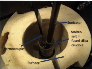
Figure 3-1: Experimental set up for dispersing the nanoparticles in molten salts... 42 Figure 3-2: Experimental set up used to measure turbidity of suspensions over a period of time.

A Laser pointer was used as the light source and a spectrometer was used to measure the

intensity of received light. Measurements were taken at periodic intervals of time... 43 Figure 3-3: Settling of 0.1 wt% titania nanoparticles in molten sodium nitrate at 350 C... 46 Figure 3-4: Settling of 0.1 wt% silica nanoparticles in sodium nitrate AT 350 0C. The

aggregation is seemingly faster than that of titania in molten nitrate and large clusters float

around in the salt... 4 7 Figure 3-5: Settling of 0.1 wt% alumina nanoparticles in molten sodium nitrate salt at 350 'C.. 47 Figure 3-6: Settling of 0.1 wt% silica particles in NaCl-KCl mixture at 750 C. The turbidity caused by silica particles in chloride salt is very high compared to that of silica particles in

nitrate salt. Also, large floating clusters of silica seen in nitrate are not seen in chloride... 49 Figure 3-7: Variation of the transmitted intensity with time for a suspension of titania

nanoparticles in molten sodium nitrate at 350 C. Initially, there is no signal due to the high turbidity of the suspension. Once the signal is obtained, it varies linearly with time, until the turbidity is low enough that the receiver saturates... 51

(8)

Figure 3-8: Variation of transmitted intensity with time of molten sodium nitrate with suspended alumina nanoparticles at 350 C. The trend is very similar to that for titania nanoparticles but the attenuation caused by alumina nanoparticles is far less than that caused by titania nanoparticles.

... 5 1

Figure 3-9: Variation of turbidity with time of a suspension of titania nanoparticles in molten sodium nitrate. The turbidity sees an exponential decay with time... 53

Figure 3-10: Evolution of attenuation area with time in a colloidal system aggregating due to Brownian collisions. The area under the lognormal curve at a given time represents the total attenuation area at that tim e ... 55

Figure 3-11: The decrease in attenuation area (or the turbidity) as a function of time, obtained by plotting the area under each curve in Figure 3-10 ... 56

Figure 3-12: Expected variation in transmitted light with time during Brownian motion

dominated aggregation. Most of the aggregation due to Brownian motion happens in the first few m in u tes... 5 7

Figure 3-13: Transmitted intensity vs time for titania nanoparticles dispersed in molten sodium nitrate at three different temperatures. The threshold value for signal decreases and the slope of the linear regime increases with temperature. There is a significant variation (increase) in the total aggregation rate with temperature. ... 58

Figure 3-14: Effect of temperature gradient on aggregation of nanoparticles. The nanoparticles aggregated close to the hotter end... 61

Figure 3-15: Transmitted intensity Vs time curves for different sized titania nanoparticles in molten sodium nitrate at 350 C. There seems to be no significant effect on the aggregation rate w ith the change in particle size... 62

(9)

Figure 3-16: Transmitted intensity Vs time (A), and turbidity vs time (B) curves for titania nanoparticles in molten sodium nitrate at 350 0C for two different concentrations. ... 64 Figure 3-17: Effect of different media on the sedimentation rates of nanoparitcles. The high temperature chloride suspension reached the threshold value before the nitrate but ended up taking more time to reach detector saturation point... 66 Figure 4-1: An example of conversion of absorption spectrum to van der Waals spectrum

through Kramers Kronig transformation. At the top, we have the F" of solid KCl, and at the bottom, we have a converted smooth monotonic van der Waals spectrum... 78 Figure 4-2: Illustration of calculation of the Hamaker coefficient using the van der Waals spectra of the materials of interest. Note that the vertical lines represent the Matsubara frequencies, over which the summation has to be carried out... 80 Figure 4-3: Effect of E" peak intensity on Lds. As the peak intensity increases, the vdW-L ds shifts upw ards. ...---. . . ---... 82 Figure 4-4: Variation of vdW-Lds with E" peak position.The vdW-Lds flattens out as the E" peak m oves tow ards right...- .. ---... 83 Figure 4-5: Effect of E" peak width on vdW-Lds with constant peak position and area under the

peak... .--- ---... 84 Figure 4-6: The E" and vdW-Lds spectra of two hypothetical materials, with significantly

different absorption properties but very close vdW-Lds ... 85 Figure 4-7: Ellisometric set up for CaF2 melt at 1823K... 88

Figure 4-8: The approximated vdW spectra for molten KCl obtained by scaling the S" spectrum of solid KCl before performing KK transformation. ... 90

(10)

Figure 4-9: Variation of Hamaker coefficient with particle separation for SiO2-KCI-SiO2 system.

The decreasing value of the Hamaker coefficient with the distance is due to retardation... 91 Figure 4-10: The E", n and vdW-Lds spectra of molten KCl at

1000*C

obtained by Ab Initio calculations using a 3X3 KC supercell cooked up at 1000 C... 93

(11)

List of Tables

Table 3-1: Estimation of Hamaker coefficient of different nanoparticles in molten sodium nitrate and molten NaCl and KCl mixture ... 45

Table 3-2: Variation of viscosity, density and perikinetic collision constant in NaNO3 with

(12)

1. Introduction

Nanofluids are stable colloidal suspensions of nanoparticles in a base fluid medium. The sizes of the particles dispersed in the liquid medium are typically less than 100 nm. These colloidal dispersions of ultra small particles are being studied the world over as advanced heat transfer fluids for various applications such as microelectronics, nuclear systems, fuel cells, hybrid powered engines etc.' It has been observed that the heat transfer coefficient in nanofluids is

2

significantly higher than that of the base fluid. The exact reasons leading to this increase in heat transfer coefficient has been a subject of great debate.3

For nanofluids to posses these superior heat transfer properties, it is important that the nanoparticles remain colloidally suspended in the medium, and do not aggregate and sediment out. In the absence of repulsive forceses between them, collisions between particles undergoing random Brownian motion leads to their sticking to one another due to the van der Waals forces of attraction between them. Also, aggregation is preferred from point of view of energetics because nanoparticles tend to minimize their surface free energy by forming large aggregates. There are two main methods of providing colloidal stability to nanoparticles in a liquid medium. Firstly, if the surface of the particles is charged, then the particles repel each other on approach, thereby avoiding aggregation. In the second method, long polymeric surfactants are attached to the surface of the particles, which hinder their approach sterically and keep them stable in suspension. These two most commonly used techniques to achieve colloidal stability are shown in Figure 1-1.

(13)

(A) (B)

Figure 1 -1: Methods of stabilizing nanoparticles in a suspension. (A) Steric stabilization, (B) Electrostatic stabilization

It must be noted that the colloidal stability is dependent on various system parameters including materials involved (both particles and medium), particle size, temperature and chemistry, as all of these influence the aggregation of particles in some way or the other. Some systems may naturally lead to charges on the surfaces of the particles and be stable without the need for any external stabilization, while others require one of the two stabilization techniques mentioned above. In this work, we intend to study the aggregation behavior of nanoparticles in molten salts at high temperatures. We will evaluate the impact each of the system parameters makes on the aggregation kinetics of the nanoparticles and investigate the possibility of making colloidally stable molten salt nanofluids in this medium. We will begin by looking into the motivation for this study and discuss some of the potential applications of high temperature molten salt nanofluids.

(14)

1.1 Motivation

The particular media that we are interested in are high melting temperature inorganic salts such as alkali halides (NaCl, KCl, LiCl etc.) and alkali nitrates (NaNO3, KNO3 etc). Molten salts are

very useful high temperature heat transfer fluids as they stay at low vapour pressures even at extremely high temperatures, thereby eliminating the need to pressurize the system. In addition, these salts are relatively low cost, are thermodynamically stable, and have high heat capacities. Consequently, molten salts, usually in the form of mixtures, are used extensively as coolants in nuclear reactors and concentrated solar thermal power plants. Nitrate salts are most often used, with the operating temperatures in the range of 250 -550 C. The peak temperatures are limited

by the chemical decomposition of the nitrate salts.

The use of chloride salts, which are stable at much higher temperatures as compared to nitrate salts, is desirable in solar thermal systems, nuclear reactors and many other high temperature engineering systems. These plants require intermediate heat transfer loops that connect the energy source to the power cycle. The heat-to-electricity efficiency increases with increasing temperatures. As such, there are large economic and environmental incentives to increase peak temperatures in these systems from the existing levels. Today, the highest-temperature commercial heat transfer fluids are nitrate salts used in various chemical plants and solar thermal power plants. The peak temperatures are between 550 and 600'C and are limited by the chemical decomposition of the nitrate salts. Higher-temperature salts made of fluorides, chlorides, and carbonates are being developed as coolants in solar power towers, nuclear reactors (advanced high-temperature reactor, molten salt reactor, salt-cooled fast reactors), and various intermediate heat transfer loops. These salts are thermodynamically stable, operate at low pressures, have high

(15)

heat capacities, and are transparent over much of the visible spectrum. While the salts have relatively low costs, the materials of construction for operations between 600 and 10000C are

expensive. The practicality of these higher-temperature systems depends partly upon efficient heat transfer that minimizes the size of heat exchangers and other equipment made of expensive materials.

Nanoparticles dispersed in molten salts can significantly alter their heat transport efficiency, as they do for any other fluid. Furthermore, at high temperatures at which molten salts operate, radiation heat transport becomes important because it depends upon the temperature to the fourth power. Nanoparticles introduced in the molten salt can conductively absorb heat from the fluid and radiate it to heat transfer surfaces. The general importance of nanoparticles in terms of heat transfer is recognized from traditional studies of particles in high-temperature combustion systems. One particular example of an application in which a dispersion of nanoparticles in molten salts can be used for efficient heat absorption and storage is the 'Concentrated Solar Power on Demand (CSpond) project, described briefly below.

1.1.1 Concentrated Solar Power on Demand

In traditional solar thermal power plants, a molten salt flows through metallic pipes. Concentrated solar rays are used to heat up the metallic pipes, which in turn transfer the heat to the salt that flows through them. The peak temperatures, as stated above, are limited by the decomposition of nitrate salts. This design has many built in inefficiencies, the major one being heat loss from non-insulated metallic pipes to the surroundings.

(16)

CSpond proposes a much more efficient design, wherein concentrated solar power will be used directly to heat up the salt, which will be maintained in a molten state in a thermally insulated tank, as shown in Figure 1-2. The molten salt can then be used as a heat storage and heat transfer fluid. Now, molten salts are usually semi-transparent and hence will not be able to absorb radiation significantly in the visible region; this is where dispersed nanoparticles can play an important role. The nanoparticles can absorb the solar energy in the visible region, and then transfer the heat to the molten salt by conduction and convection. This will result in the heat being absorbed over the entire volume of molten salts, and the heat from the otherwise wasted visible part of the solar spectrum would be utilized efficiently.

Solar Rays

Aperture

Ground

Salt from/to

Salt with _{heat generation loops}

nanoparticles

Figure 1-2: The basic model design of CSpond. Solar rays enter directly into the molten salt, where they are absorbed by the dispersed nanoparticles.

Sandia laboratories have studied the effect of nanoparticles on absorptivity of molten salts, and found that 0.1 wt% of nanoparticle dopants can enhance solar energy absorbed per centimetre of fluid depth from 8% to 90%.4 Thus, the utility of dispersed nanoparticles in molten salts has been

(17)

established. However, to the best of our knowledge, no attempt has ever been made to study aggregation propensity and colloidal stability of nanoparticles in molten salts. It is important to realize that for any engineering benefit to be gained by exploiting the use of nanoparticles in molten salts, the problem of colloidal stability is of utmost importance. Besides, even if particles are not intentionally added, they can be present (or generated) in the system as impurities, and it is important to understand their colloidal stability to determine the potential impact of such impurities on the heat transfer properties of the salt.

1.2 Methodology and approach

As stated above, the goal of this project is to study the colloidal stability of various nanoparticles in the molten salt medium and evaluate the possibility of developing kinetically stable nanofluids in these environments. Because of the high temperatures (- 1000C) and high thermal energy, the requirements for engineered nanoparticles in these systems are more severe than are those for nanoparticles in lower temperature fluids. However, before moving into the main problem of colloidal stability, we need to bear in mind a few other constraints that limit our choices of nanoparticles that could be appropriate for this high temperature system. Firstly, it needs to be ensured that the nanoparticles are physically and chemically stable in the medium. For physical stability, one needs to choose particles that won't soften and deform at temperatures in the range of 1000 0C. Thus, only high melting point ceramics can be considered. Also, for chemical

stability, it needs to be ensured that the nanoparticles do not react chemically with the molten salts at the temperatures of interest. Furthermore, the nanoparticles also need to be extremely insoluble in the salt medium in order to avoid particle coarsening due to Ostwald ripening. Few candidate materials that satisfy this criterion are high temperature ceramics such as silica (M.P.

(18)

1650 *C), alumina (M.P.2072 "C), titania (M.P. 1843'C), etc. In fact, these are the most common

materials used for most high temperature applications.

Now, this leaves us with our main problem of colloidal stability. In order to evaluate the potential development of dispersed nanoparticles that can provide strong thermal absorption and radiant emission for enhancement of heat transfer rates within molten salts, we will have to study the colloidal behaviour of the nanoparticles in this medium in some detail. Both low temperature nitrate salts (250-550 0C) and high temperature chloride salts (550-1000 0C) will have to be

considered. We will first begin by looking into the fundamentals of particle aggregation and deposition in a general colloidal system, and understand in detail the processes and parameters that determine the colloidal stability in any dispersion. We will look into the peculiarities of our medium (high temperature, ionicity etc) that introduces difficulties in obtaining a stable dispersion of nanoparticles, and evaluate the parameters that we expect would theoretically make an impact on colloidal stability. We will then experimentally study the rate of deposition of nanoparticles in molten salts, and its variation with important parameters such as materials, temperature, concentration etc. Finally, based on the theory and experimental observations, we will evaluate the possibility of engineering a system which can remain colloidally stable.

(19)

1.3 References

1. Das, S., Nanofluids: Science and Technology. Wiley Interscience: 2007; p 397.

2. Kakac, S.; Pramuanjaroenkij, A., Review of convective heat transfer enhancement with nanofluids. International Journal Of Heat And Mass Transfer 2009, 52, (13-14), 3187-3196.

3. Buongiorno, J., Convective transport in nanofluids. Journal of Heat Transfer (American Society of Mechanical Engineers) 2006, 128, (3), 240.

4. Drotning, W. D., Optical-Properties Of Solar-Absorbing Oxide Particles Suspended In A Molten-Salt Heat-Transfer Fluid. Solar Energy 1978, 20, (4), 313-319.

(20)

2. Theory of colloidal stability and aggregation kinetics

2.1 Interactions between particles in a colloidal system

The interaction forces between the particles that are primarily responsible for the behavior of the colloidal systems, in particular, their colloidal stability, are usually those of electrostatic repulsion and van der Waals attraction. In addition, hydration and steric forces can also come into play in the system and make a significant impact on colloidal stability. We describe briefly

the origin and the impact of each of the forces in the system of our interest in this section.

2.1.1 Electrostatic repulsion

In many colloidal systems, repulsive electrostatic interactions between the particles play the most important role in providing colloidal stability to the particle suspension. If the colloidal particles are charged, they tend to repel one another and prevent particle aggregation (and eventual sedimentation), thereby ensuring colloidal stability. Many particles naturally develop a charged surface in a particular medium. There can be several origins of such a charge on the surface, one example being that of metal oxides like SiO2, A1203, TiO2, Fe2O3 etc. in an aqueous medium. In

contact with water, the oxide surface becomes hydroxylated, thereby resulting in either positive or negative surface charge, depending on the pH. The ionization of such groups can be represented as shown in Figure 2-1.

(21)

OH₂

Uri'

0-H~

O-Figure 2-1: Development of a charge on oxide particles in aqueous medium due to hydroxylation

At higher pH, the equilibrium is driven towards right, as the surface tends to lose protons and become negatively charged, whereas at lower pH, the equilibrium is driven towards left and surface is positively charged. The kind of charge that gets developed at a particular pH depends on the nature of the material. For acidic oxides like silica, the charge is negative for most of the

pH range, while basic oxides like MgO are positively charged at most pH values. Besides

hydroxylation at the surface of the colloidal particle, a charge might also arise naturally due to several other factors driving thermodynamic equilibrium between the particle and the medium.' In addition to that, surfaces can also be intentionally charged by chemically attaching charged groups onto the surface, in order to enhance the colloidal stability.

At this stage, in order to understand the electrostatic interactions between the particles in a better way, it is also important to understand the concept of an electrical double layer. The charge on the surface of a colloidal particle is exactly balanced by an equal and opposite charge in the solution near the surface, resulting in the formation of an electrical double layer.' The first layer (called as stem layer) consists of the fixed charges close to the surface of the particle which are all of the opposite charge to that of the particle, and hence strongly attracted towards the particle. The second layer (called the diffuse layer) consists of mobile charges which are at some distance

(22)

away from the particle. The typical electrical double layer and the variation of potential as a function of distance for the case of a colloidal particle with a charged surface in a medium with dilute concentration of ions are shown in the Figure 2-2.

For two spheres of equal radius, the electrostatic interaction potential is given by

VR = 32TEa 2 2 exp (-Kh) (2-1)

Where , is the dielectric permittivity of the medium, k is the boltzman constant, T is the

temperature, z is the ionic concentration in the medium, e is the electronic charge, y is the function of dimensionless surface potential, K is the Debye Huckel parameter and h is the

distance between the particles.2

The characteristic parameters that describe the double layer are the zeta potential ( and the Debye huckel parameter K, which has the dimensions of reciprocal length, and is given by

C2 _2e ckTz noZ2

(2-2)

ekT

The inverse of the Debye Huckel parameter (1/K) is a measure of the thickness of the diffuse layer and is also known as Debye length. At a distance 1/K from the surface, the potential has fallen to a value l/e of the surface potential. Thus, the Debye Huckel parameter is a measure of the extent of counterion charge in the diffuse layer. 1/K is indicative of the range of electrical interaction between the particles. The smaller the Debye length, the smaller will be the double layer thickness and consequently, smaller will be the range of the electrostatic interaction between the particles. As we can see from the Equation 2-1, the interaction potential decays

(23)

exponentially with distance, with a decay length of 1/K. The potential due to the surface charge at the end of stern layer is called the stem potential and the potential at end of diffuse layer is called zeta potential. Thus, zeta potential is the potential difference between the dispersion medium and the edge of the diffuse layer. At constant ionic strength of the medium, higher the charge on the particle, higher will be the zeta potential. zeta potential and the Debye length are the parameters that are used to characterize the strength of electrostatic interactions between the particles.

Electrical double

layer

Slipping plane

Particle with negative surface charge

I I I I

Stern layer| Diffuse layer

-100 I I I '$suface poten&IaI I: ZWMa mv

0'

Distance from particle surface

Figure 2-2: Schematic of the electrical double layer (EDL) formed across a negatively charged colloidal particle. Image Source:

(24)

Now, consider what happens when we add salt to an aqueous colloidal dispersion. In general, an increase in the ionic concentration of the system leads to a decrease in the magnitude of the zeta potential ( and also in Debye length 1/K. Both of these lead to a decrease in the repulsion between the particles. Thus, ions in the system screen off the coulombic interactions between the particles.

Now, the medium that we are dealing with, i.e. molten salts has an extremely high concentration of ions. As a result, the Debye length becomes extremely small, and the electrostatic interactions are more or less completely screened off. It is important to note that the classical analogy (of decreasing Debye lengths and zeta potential) cannot be applied to the systems where ionic concentration is as high as in the case of molten salts, and some modifications need to be made. Firstly, in case of ionic liquids, the ions are not independent of one another, and the ion correlation effects can be quite strong. Thus, a correction factor has to be brought in when determining the effective charge concentration in the medium if Equation 2-1 is to be used. More importantly, the arrangement of charged ions close to a charged surface in molten salts is actually very different from the double layer model described above for dilute aqueous electrolyte solutions. The theory of electrical double layers has been built by placing a restriction on ion volume, and cannot be directly extended to the molten salts. In a molten salt, the screening of charges is not exactly due to oppositely charged ions in the double layer, and the potential does not decay exponentially with distance. A lot of research is currently being carried out to understand the structure and dynamics of ions at the charged surface in a molten salt medium.3 _{Computer simulations have indicated pronounced and long range charge density}

oscillations close to the interface.4 _{Figure 2-3 shows the potential across a cell consisting of}

(25)

624 40f - OJ.0 40.0 --- 8,0' 20 32.0 J4 -20~* 0 2 4 6 8 10 12 14 16 18 20 22 24 26 28 30 Z, nm

Figure 2-3: The variation of potential with distance between electrodes with different surface charge densities in an ionic liquid cell. The potential profile differs significantly from the exponentially decaying one observed in the case of an electrical double layer.4

The main take away from the Figure 2-3 is the fact that the charges are screened efficiently by molten salts and the effect of the charged surfaces is completely neutralized. The screening of charges takes place due to local polarization of the high density layers at the surface. One of the important results arising from the difference in screening mechanism is that molten salt responds far more quickly (-3 orders of magnitude) to changes in surface charge densities than a traditional electrolyte using double layer mechanism would.5 _{Thus, it is actually much more}

efficient in screening off the electrostatic interaction between charged colloidal particles. In a nutshell, even though the theory of the double layer has to be built completely differently for molten salts, the bottom line remains that the electrostatic interactions are screened off

(26)

completely by the constituent ions and charged colloidal particles are unlikely to face any repulsion when they approach one another.

2.1.2 van der Waals forces

Another very important interaction between the colloidal particles is the van der Waals force of attraction, which, in general, has three components, viz, Keesom, Debye and London forces. The Keesom force is the force of attraction between two permanent dipoles. The Debye force is the force of attraction between a permanent dipole and an induced dipole. The London force is the force that always occurs between the particles (even if there are no permanent dipoles), and is caused by spontaneous oscillations of electron clouds which generate temporary dipoles. These temporary dipoles induce temporary dipoles in neighboring atoms, and the resultant force of interaction between these two dipoles is the London dispersion force. In colloidal systems, when we talk about van der Waals forces between two colloidal particles, we essentially mean the ever-present London dispersion force. From now on, van der Waals forces and London dispersion forces will be used interchangeably in this text.

The van der Waals energy between two particles depends upon the geometry of the two particles and the Hamaker coefficient for the system. For two spherical particles of equal sizes (diameter d and distance s between the particles), the van der Waals energy of interaction is given by Equation 2-3.6

UvH (2-3)

1 1 x2+2x

where

H(x)

= + 1

+

2n(

)

(2-4)

(27)

The Hamaker coefficient, A, can be shown theoretically to depend upon the variation with wavelength of the complex dielectric constant of the particles and the medium. To a certain extent, it can be estimated from the refractive indices and the static dielectric constants of both particle as well as the medium.

It is not immediately intuitive that van der Waals forces of attraction depend on properties like refractive indices of the materials involved. However the intuition comes when we delve into the origin of the force. As described above, London -van der Waals forces are created by collective coordinated interactions of oscillating electric charges. They result from charge and electromagnetic field fluctuations at all possible rates. Now, frequencies at which charges spontaneously fluctuate are the same as those at which they naturally move, or resonate to absorb external electromagnetic waves. This fact helps us to understand the inherent connection between the van der Waals forces and the electromagnetic properties of the materials involved. Lifschitz developed the modern theory for estimation of the Hamaker coefficient in terms of the properties (dielectric spectrum or the absorption spectrum) of all the materials involved in the medium.7

Thus we see that in order to estimate the Hamaker coefficient, we need to know the material of the nanoparticles and the medium. The Hamaker coefficient between two particles of material 1, in a medium 2, is represented as A121. When the Hamaker coefficient of a material is stated

without specifying the medium, the medium is implied to be vacuum by default.

The data required for precise determination of Hamaker coefficients are difficult to obtain, (though possible nevertheless). Theoretically, the dielectric response over the entire frequency range from zero to infinity is required. However, for all practical purposes, accurate estimation of the Hamaker coefficients using the full spectral formulation of Lifschitz can be made if

(28)

relevant dielectric data are available for 0 to 40 eV. As even this information is rarely available, most estimation of Hamaker coefficients are based on approximations, which use just the visible refractive index of the materials involved, instead of the entire spectrum over all the wavelengths. Equation 2-5, known as the Tabor Winterton Approximation (TWA) gives the approximate value of the Hamaker coefficient.8

ArA _ 3rnve (niso,- n2iso,2)

(2-5

8V2(n 2,+ n22

Where,

A2 = The Hamaker constant for 'material 1' with 'material 2' as the medium, 2

naso = Visible refractive index of 'material 1' in vacuum 2

nv,so,2 = Visible refractive index of 'material 2' in vacuum Ve plasma frequency ~ 3*1015 Hz for ionic liquids

h = Planck's constant

Another important empirical approximation is widely used for estimation of the Hamaker coefficient of particles of material "1" in medium "2", if the Hamaker coefficient in vacuum is known for materials of both the particles and the medium.

The Hamaker coefficient of the particles "1" interacting across the medium "2" is given by

A

1 2 1 =

(A2

-

A

2

(2-6)

An important point to note is that the Hamaker coefficient itself depends on the distance between the particles. If the particle distance increases, the coordinated motion of the charges

(29)

between the two interacting particles falls out of sync which leads to reduction of the Hamaker coefficient. This effect is known as retardation. When the interacting particles are in contact, we have the non retarded Hamaker coefficient, which is constant for the given particles and the medium and hence also known as the Hamaker constant. Henceforth in this document, unless otherwise mentioned, the term Hamaker coefficient will mean the non-retarded Hamaker coefficient. We will discuss the full spectral lifschitz formulation for obtaining the Hamaker coefficients in Chapter 4.

It must be noted that in principle, the interaction energy (and force of attraction) due to london van der Waals forces will become infinite at contact, as suggested by 2-3. This, as we know is obviously not the case. If it was, it would be impossible to break clusters of particles by stirring or sonication. At very close approach, short range repulsion forces like Born repulsion come into the picture, and prevent the separation distance from becoming absolutely zero. The equilibrium separation distance between the particles apparently in contact is normally between 0.1-0.2 nm.9 This finite distance ensures that the van der Waals force too remains finite. Furthermore, the roughness of the surface will also play an important role in limiting the minimum separation distance between the particles. We will revisit this particular concept and evaluate the possibility of using this to our advantage in chapter 4.

2.2 DLVO theory of colloidal stability

In section 2.1 we considered in some detail two of the most important forces of interaction between colloidal particles, which are largely responsible for determining the colloidal stability. These forces form the basis of the DLVO theory of colloidal stability, developed by Derjaguin and Landau (1941)10 and Verwey and Overbeek (1948)."

(30)

DLVO theory is a well established framework that considers total interaction energy between any two particles as a function of particle separation and helps to predict whether or not a particular suspension will be colloidally stable. Essentially, the total energy of interaction between the particles is simply given by the addition of the van der Waals attraction and the

electrical double layer repulsion. Thus,

UT = UdW + UEDL (2-7)

The variation of interaction energy with distance between the particles can take several different forms, depending upon the relative strengths of various parameters such as particle size, zeta potential, Debye length and Hamaker coefficient that determine the van der Waals and electrical double layer interactions. The typical shape of the DLVO curve for most colloidal systems is presented in Figure 2-4 below. As shown, the vdW force of attraction and EDL force of repulsion together result in one maximum (called the primary maximum), and two minima (primary and secondary minima). The shape of the "net" DLVO potential determines the colloidal stability and the aggregation rate of the particles. The primary maximum represents an energy barrier that needs to be crossed if the two approaching particles are to come in contact and agglomerate. The higher the barrier, the lower will be the aggregation rate, as more particle-particle approaches will be repelled due to the barrier. In a colloidal system, the kinetic energy that approaching particles have is due to the Brownian motion. The energies of the particles follow a Gaussian distribution with kT as the mean. If the particles are charged, the strong electrostatic repulsion force between the particles will ensure a large energy barrier, which would lead to a colloidally stable system.

(31)

Primary Minimum

C

0

-tSecondary Minimum Particle Separation

Figure 2-4: A typical DLVO potential curve. It is the summation of the elctrostatic and van der Waals interaction energy, which results in a one maximum and two minima.

Again, it is important to note that in principle, the van der Waals force will be infinitely strong at contact and the primary minimum will be infinitely deep. This will mean that no two particles which come in contact could ever be separated. However, the short range Born repulsion forces, hydration effects and surface roughness all combine to ensure that the attraction force (and hence the depth of primary minimum) remains finite. So if a breaking energy greater than the depth of the primary minimum is provided to a two-particle aggregate, the aggregate would disintegrate into its individual constituent particles. The secondary minimum brings in a few more nuances in the aggregation process in some colloidal systems, and can be responsible for weak large range aggregates. For now, we will neglect the effects of the secondary minimum because it does not play any significant role in the system of our interest.

The parameter that determines the colloidal stability is the collision efficiency (or sticking coefficient) a, which is the fraction of particle collisions that lead to sticking. As should be obvious by now, the value of a depends on the DLVO profile. The reciprocal of a is called the 20

(32)

stability ratio W, which is the ratio of aggregation rate in absence of colloidal interactions to that found when there is repulsion between the particles. For a purely DLVO system (neglecting hydration effects, which will be discussed later), an expression was derived for the stability ratio

by Fuchs by treating the problem as that of diffusion in a force field. The expression for W is

given in Equation 2-8.

W

= 2

00

exp (/kT

du

(2-8)

0 (u+2)2

where (DT is the total interaction at a particle separation distance d. u is a function of d and

particle size. For spherical particles of different radii ai and aj, u is given by

U 2d (2-9)

ai+a;

For equal sized particles this just becomes u=d/a. Reerink and Overbeek made an approximation

by making use of the fact that the region close to the maximum contributes a large portion of the

integral.13 Equation 2-8 then gets reduced to

W = exp (<Pmax/kT) (2-10)

x(ai+a)

In Equation 2-10, the stability ratio just becomes a function of the Debye length and the barrier height, rather than the entire DLVO profile. From Equation 2-10, we find that for ionic concentration of 0.1M and particle size of 1 m, if the barrier height is 20 kT, roughly one in a million approaches will have the energy to cross the barrier. Equation 2-10 helps us to easily

(33)

connect between the barrier height and the collision efficiency. So far we have been talking about the general colloidal system. However, as we saw earlier, the system of interest is quite unique because of the fact that all the electrostatic charges are completely screened. So, the DLVO potential profile of particles in molten salt medium will not exhibit an energy barrier. We can see the effect of increasing salt concentration on the height of the DLVO primary maximum in Figure 2-5.14 It shows how the DLVO potential of gold nanoparticles dispersed in water is affected by increasing salt concentration in water. As the concentration increases, the EDL interactions between the particles decrease and consequently, the DLVO energy barrier decreases. As can be seen, at IM NaCl concentration there is hardly any energy barrier to prevent the agglomeration of gold particles. When the value of the primary maximum becomes zero, i.e. when the energy barrier disappears completely, the sticking coefficient ideally will become equal to 1. 40-30. 1M 20. 0.03 M 10 0.1 M 0..0.3... 0.3 M -10. 1 M 0 2 4 8 10 Distance (nM)

Figure 2-5: Variation of DLVO energy barrier with increasing salt concentration. As the salt concentration increases, the energy barrier decreases due to the screening of electrostatic interactions14

(34)

The number of ions in a molten salt will be much higher than those in 1M salt solution. In fact, as we saw earlier, molten salts are much more efficient in screening the charges than an aqueous electrolyte of similar ionic conductivity. Hence it is reasonable to expect that the DLVO energy barrier will completely disappear when the medium of dispersion is a molten salt, as is indeed the case. Figure 2-6 compares the DLVO energy barrier for charged silica particles in 0.1 M 1:1 salt aqueous solution and that in different ionic liquids. As can be seen, the DLVO energy barrier disappears when charged silica is dispersed in an ionic liquid.15

-5Ionic Liquid -[C4rn][NTI2] --- [C4mim][BF4] [C4miM][PF6] 10 -0.1 M 1:1 salt s. - Iaqueous system .5 0 1 2 3 di nm

Figure 2-6: Effect of charge screening by ionic liquids on the energy barrier'5

The variation of stability ratio with increasing ionic concentration in a medium is of interest. As shown in Figures 2-5and 2-6, the DLVO energy barrier decreases with increasing salt concentration in an aqueous system. This will lead to a decreasing stability ratio and increasing sticking coefficient. Figure 2-7 presents a schematic diagram showing the effect of increasing salt concentration on stability ratio.' On a log-log plot, the variation of the stability ratio with the

(35)

salt concentration is linear. However, the stability ratio does not decrease indefinitely as the salt concentration is increased. When the salt concentration is high enough to suppress the potential barrier completely, further increases in salt concentration do not lead to any significant change in stability ratio. This concentration at which the barrier disappears is known as critical coagulation concentration (CCC). After this concentration, the stability ratio becomes equal to 1 and all collisions lead to aggregation.

log

W

ccc

_log

_C

Figure 2-7: Variation of stability ratio with salt concentration. The stability ratio initially decreases linearly with increasing salt concentration, and becomes constant after reaching the critical concentration. 1

(36)

The fact that the stability ratio does not decrease beyond the CCC has an important consequence for our system consisting of a molten salt medium. CCC represents the point where the primary maximum becomes zero. Even beyond the CCC, increasing salt concentration will still keep lowering the primary maximum into the negative, as we can see in Figure 2-5. In other words, attraction between the particles will keep increasing with increasing salt concentration after the

CCC, until the net DLVO curve coincides completely with the van der Waals attraction curve.

However, this attraction between the particles is rarely sufficiently long range to have any significant impact on the collision frequency. That is to say, the collision frequency is largely dominated by the Brownian motion, and hence depends mainly on the diffusion coefficient of the particles. The rate of aggregation is simply the rate of collisions times the collision efficiency (or sticking coefficient). Brownian motion determines the collision rate, and the DLVO forces determine the sticking probability. Thus, we can say that aggregation rate will only depend upon the colloidal interaction when there is repulsion between the particles. In that case, not all collisions will lead to aggregation, and the collision efficiency will depend upon the Hamaker coefficient, Debye length and zeta potential. But once there is no repulsion between the particles, the aggregation rate depends very little on how strong the van der Waals interaction is between the particles. In the case of molten salt, the EDL interaction between the colloidal particles will be completely suppressed due to total screening of charges. Thus, if we only consider the effect of DLVO forces and neglect the hydration and viscous effects, the Hamaker coefficient is expected to have very little effect on the aggregation rate of nanoparticles.

(37)

2.3 Non DLVO forces: Hydrodynamic effects

The DLVO theory does not take into account effect of viscosity of the medium. These effects can sometimes play a significant role in determining the aggregation kinetics. Due to the no slip condition at the boundary, the liquid between the particles does not drain out easily which slows the aggregation process. In other words, the diffusion coefficient is reduced as particles approach each other due to the hydrodynamic interaction between the particles. No slip condition at the interface makes the diffusion coefficient approach zero as the particles come into contact. Ideally, in such a case, the particles would never aggregate. However, the van der Waals attraction between the particles brings them together by negating the viscous resistance at close approach. Quite clearly, van der Waals forces become more important in determining the aggregation rate when we do take into account the hydrodynamic interactions between the particles. Honig 16 reported an empirical approximation for the variation of the diffusion coefficient with particle separation for an aqueous suspension.

D(u) _ 6u2+4u _ 1

D(o) 6u2+13u+2 ft(u)

Here,

u - dimensionless distance u=d/a

D(u) - diffusion coefficients for particles separated by distance u D(oo) - diffusion coefficients for particles at infinite separation

p(u)

is a correction factor that needs to be applied between every pair of particles. Physically, it means that the diffusion coefficient is reduced at a separation u by this correction factor. The

(38)

impact of viscous effects can be fairly long range. Equation 2-11 has been developed for water. The extent of hindrance these hydrodynamic effects provide depends not only on the physical properties such as the viscosity of the medium, but also on the nature of bonding close to the particle surface. Adhesive water layers form close to the surface of the particles due to hydrogen bonding between water molecules. The description of

P(u),

hence will be different for different media. The example of water, can however be used as a general reference for qualitative

arguments.

If we correct for the hydrodynamic interactions in the equation for stability ratio, we get:

ooexp Tg7T

Wum =J 2J (uI) (+2kT) du (2-12) Wvv1LmL.=J2Ifo l (U (u+2)2

In the case of an electrically fully destabilized system (like particles in molten salts), 9T will just be the van der Waals interaction energy. One can now obtain the variation of stability ratio with Hamaker coefficient for the case of water, with and without taking into consideration the hydrodynamic interaction.

(39)

E

-I ---- --- - -

--0.1 1 10 100 1000

Hamaker ConsaW"O- 3

Figure 2-8: Variation of limiting stability ratio versus the Hamaker coefficient taking into consideration the hydrodynamic interactions (Solid line). The dotted line shows the variation when hydrodynamic interactions are not considered.'

As we see in Figure 2-8, the limiting stability ratio varies significantly with Hamaker coefficient when the hydrodynamic effects are taken into consideration. The stability ratio for particles with Hamaker constant 1 zJ is approximately twice that at 100 zJ. Most colloidal materials will fall within this range of Hamaker constant. Also, as discussed before, when only DLVO forces are considered, the variation is little and unlikely to result in any significant change in aggregation rate.

(40)

2.4 Smoluchowski model of aggregation kinetics

Having considered the nature of different interactions in a colloidal system, we turn our attention to the models for aggregation rates. Smoluchowski first developed a model for the aggregation process in 1917.'1 It is regarded as a classic work in the field and is still the starting point of most discussions on aggregation. The model is based on the assumption that the rate of collision between two sizes of particles is proportional to the concentration of the particles with those sizes. So, if there are ni particles of size i and nj particles of size

j,

then the number of collisions occurring between them in a unit time and unit volume will be given by Equation 2-13.

Jij

=

kijninj

(2-13)

Here kij depends on various factors like particle size, fluid properties, and the dominant mechanism of aggregation. Also, it is important to note that in this model, aggregation is assumed to be a second order process, and three (or more) body collisions are ignored.

When all collisions produce aggregates, as is likely in the case of molten salts, the aggregation rate is the same as the collision rate. When there is a repulsive interaction between the particles, or when the hydrodynamic hindrance is significant, we need to take into account the collision efficiency a, which is just the inverse of the stability ratio. In this case, the rate of aggregation is

Jij

=

aktjninj

(2-14)

In the smoluchowski model, the particles are assumed to coalesce and form a bigger spherical particle with a volume equal to the total volume two colliding particle. While this assumption is

(41)

not strictly valid except in the case of liquid droplets, it is still found to yield reasonable estimates of aggregation kinetics of particles in an isotropic field.

Now, the effective rate of creation of k sized particles can be written as:

dt 1 ,->k- kijninj - nk

x*=

1 kikni

(2-15)

The first term represents creation of k sized particles from two smaller sized particles of sizes i and

j.

The second term represents destruction of a k sized particle due to its agglomeration with another particle to form a bigger particle.

While Equation 2-15 has been derived with discrete particle sizes in mind, an equivalent form for continuous particle size distribution has been established by G. M. Hidy.18 The integral form is shown in Equation 2-16.

't =

fo

k (i

-

j, j)n(j, t)n(i

-j,

t)dj

-

n(i, t)

f7

k(i, j)n(j, t) dj

(2-16)

2.4.1 Mechanisms of collisions

The main parameter that needs to be evaluated in order to make use of Equations 2-15 and 2-16 is the collision rate kij, which depends upon the dominant mechanism of collision. The process of aggregation can take place through three main dominant mechanisms, viz. perikinetic

(42)

aggregation, orthokinetic aggregation and differential settling. The value of collision constant k depends upon the mechanism of collision.

2.4.1.1 Perikientic Aggregation

Perikinetic aggregation is dominated by Brownian motion and the resultant collisions between the particles. This is the dominant mechanism for nanoparticles in stationary fluid, as the force of gravity is negligible in comparison to Brownian force. The rate constants for perikinetic

collisions is given by Equation 2-17.1

= 2kT (ai+aj)2 (2-17)

311 aja;

Where

kT - Thermal energy

p- viscosity

ai, ai - sizes of the colloiding particles

For equal sized particles, the expression reduces to

k = 8kT (2-18)

3y

2.4.1.2 Orthokinetic aggregation

Orthokinetic aggregation occurs due to collisions of particles brought about by motion of the fluid (due to flow, stirring etc.) which can lead to enormous increase in the rate of interparticle collisions. In our case, we will be mainly dealing with a stationary molten salt, so the

(43)

orthokinetic component will come only from any convective currents that exist in the system. In such a case, without any apparent flow of the fluid medium, the contribution of orthokinetic aggregation is expected to be insignificant compared to perikinetic aggregation. Also, shear forces acting on aggregates can also lead to breaking of aggregates, which needs to be taken into account when dealing with Orthokinetc aggregation. The collision rate constant in this mode of transport is given by Equation 2-191.

k

i

=4

G

(ai+aj)2

(2-19)

3 aja;

2.4.1.3 Differential settling

The third important collision mechanism is when larger particles settling under gravity collide with slower settling smaller particles on their way. This normally becomes the dominant mechanism of collision when particle sizes are large enough to be affected by gravity (typically of the order of 10 p). The collision rate constant when differential settling is dominant is given

by Equation 2-20'.

k

(1

) (p, - p)(ai ±

a)

3(at - aj) (2-20)

For our problem, when nanoparticles are dispersed in a molten salt, we expect that the particles would initially aggregate due to Brownian collisions whereas later, when larger clusters are formed, differential settling collisions will be the primary mechanism.

(44)

2.5 Studies of colloidal stability in Ionic liquids

There are factors beyond DLVO forces that can play a very important role in determining the aggregation rate of colloidal particles in various systems. Hydration and solvation forces can depend greatly upon the interface characteristics of the system. The closest system comparable to molten salts that have been studied in some detail in the literature are ionic liquids. Ionic liquids are, in principle molten salts, but they liquefy at room temperature. However, the ions which are present in these room temperature liquefying salts are of a different kind. They mostly contain at least one organic ion, which is significantly greater in size as compared to inorganic ions such as alkali ions, halides, or even nitrates. While the basic fundamental properties like charge screening remain pretty much the same in ionic liquids and molten salts, there can be several effects due to the large size of the ions which could alter the aggregation behavior of colloidal particles in the two media. If we just go by the DLVO forces, all bare nanoparticles will agglomerate rapidly in ionic liquids, as there will not be any repulsion between the particles. Thus any attempts of electrostatic charge stabilization are likely to fail. However, some transition metal nanoparticles like gold show very good colloidal stability in ionic liquids even in the absence of stabilizers or polymers.19 Even silica nanoparticles have been found to show greater colloidal stability than expected in a completely destabilized system.20 Detailed understanding of stabilization or aggregation of nanoparticles in ionic liquids has not yet been achieved, and it is an active area of research. However, one of the important factors is steric hinderance derived from adsorption of the bulky ions of the ionic liquid. These ions are large enough to separate colloidal particles by forming protective layers in the presence of strong binding interaction between the ionic liquids and the colloidal surface. Another phenomenon that is believed to affect colloidal stability is formation of a structured hydration layer at the particle surfaces by

Colloidal stability of magnetic nanoparticles in molten salts