HAL Id: hal-01480263
https://hal.archives-ouvertes.fr/hal-01480263
Submitted on 13 Mar 2017
HAL is a multi-disciplinary open access
archive for the deposit and dissemination of
sci-entific research documents, whether they are
pub-lished or not. The documents may come from
teaching and research institutions in France or
abroad, or from public or private research centers.
L’archive ouverte pluridisciplinaire HAL, est
destinée au dépôt et à la diffusion de documents
scientifiques de niveau recherche, publiés ou non,
émanant des établissements d’enseignement et de
recherche français ou étrangers, des laboratoires
publics ou privés.
Unsteady dynamics of PAH and soot particles in
laminar counterflow diffusion flames
Pedro Rodrigues, Benedetta Franzelli, Ronan Vicquelin, Olivier Gicquel,
Nasser Darabiha
To cite this version:
Pedro Rodrigues, Benedetta Franzelli, Ronan Vicquelin, Olivier Gicquel, Nasser Darabiha. Unsteady
dynamics of PAH and soot particles in laminar counterflow diffusion flames. Proceedings of the
Com-bustion Institute, Elsevier, 2017, 36 (1), pp.927 - 934. �10.1016/j.proci.2016.07.047�. �hal-01480263�
Unsteady dynamics of PAH and soot particles in laminar counterflow di↵usion
flames
Pedro RODRIGUESa,⇤, Benedetta FRANZELLIa, Ronan VICQUELINa, Olivier GICQUELa, Nasser DARABIHAa
aLaboratoire EM2C, CNRS, CentraleSupélec, Université Paris-Saclay,
Grande Voie des Vignes 92295 Châtenay-Malabry Cedex, France
Abstract
Due to their low chemical time scales, the production of soot particles in turbulent di↵usion flames is highly impacted by large range of local strain rate fluctuations.
In order to understand the response of soot production to strain rate fluctuations, unsteady laminar counterflow di↵usion flames with an imposed oscillating strain rate are investigated both analytically and numerically. First an analytical linearized model is developed to predict the unsteady response of a flame quantity of interest from information on laminar steady flames. Three critical parameters governing flame response are identified: the Stokes number which compares the characteristic time associated to the mean imposed strain rate to the oscillation frequency, the Damköhler number associated to the quantity of interest, and a third one characterizing the response of this quantity to an imposed steady strain rate. This model is then applied to soot predictions. Parallely, the response of soot production in propane-air counterflow di↵usion flames to unsteady strain harmonic oscillations is studied numerically using a detailed sectional soot model. A wide range of frequencies and amplitudes are considered. A specific trend is highlighted for soot precursors and particles production according to their respective chemical time scales: the bigger the PAH or soot particle, the higher its chemical time scale, resulting in a more damped and phase-lagged response. The particle size distribution evolves accordingly during the considered oscillations, so that the quasi-steady state behaviour is not verified for high frequencies. The numerical results are compared to those obtained by the analytical approach and a very good agreement is obtained at low amplitudes. Non-linear response of soot precursors and soot particles production to strain oscillations are finally discussed in case of high oscillation amplitudes and the limits of the proposed analytical model are identified.
Keywords: Soot, PAH, Laminar flame dynamics, Soot sectional model, Particle size distribution 1. Introduction
Due to incomplete combustion, soot emissions have e↵ects on both human health and environment. Soot emissions are also considered as an important cause of
global warming [1]. Consequently, important e↵orts are
made both experimentally and numerically [2,3,4] to
understand soot production mechanisms in order to con-trol their emission.
Most of the combustion facilities are characterized by high Reynolds number flames where turbulent eddies are expected. The local strain rate usually fluctuates in a
⇤Corresponding author:
Email address: pedro.rodrigues@centraliens.net (Pedro RO-DRIGUES)
wide amplitude range and with random fluctuation
fre-quencies [5]. These turbulent eddies are also
responsi-ble for variaresponsi-ble length scale recirculation zones, intro-ducing a wide range of residence times for soot parti-cles, strong intermittency and dynamics features in soot
production [6,7].
One of the most popular approaches used to simulate turbulent non-premixed flames is the flamelet approach, based on a quasi-steady response of the flame
character-istics to the local strain rate fluctuations [8,9].
In the optic of applying such models to numerical simulations of turbulent flames, the response of soot to strain rate fluctuations can be investigated by look-ing at unsteady laminar counterflow di↵usion flames
[10,11,12]. Specifically to soot context, previous
laminar flame by introducing sinusoidal velocity
vari-ations at both opposed nozzles [13,14] . They showed
that soot production response to these fluctuations was phase-lagged and damped when increasing the oscilla-tion frequency. A particular hierarchical behavior was observed: soot volume fraction response is more phase-lagged and damped compared to soot precursors re-sponse, which are also more phase-lagged and damped
than the temperature response [15]. Cuoci et al. [16]
numerically investigated these flames with good predic-tion of unsteadiness soot dynamics, confirming the ex-perimental observations. Nevertheless, a lack of knowl-edge remained on the origin of soot response to un-steady strain fluctuations. Moreover, when computing counterflow di↵usion flames with unsteady velocities at the nozzle exits, a phase lag exists between the global
strain rate and the local strain rate [16], increasing the
complexity of the phenomena.
The objective of the present work is to characterize the response of soot to strain rate oscillations and to identify the physical phenomena underlying the phase lag and damping observed in soot production. In order to avoid the phase lag between the global and the local strain rate, a strain-imposed formulation is considered in this work and unsteadiness is introduced by varying the imposed flame strain rate a(t) with time for a given
pulsation !, an initial strain rate A0and fluctuation
am-plitude a1:
a(t) = A0+a1sin(!t) = A0⇥1 + ↵sin(2⇡ft)⇤. (1)
Both analytical and numerical approaches are consid-ered in this paper to study the evolution of the soot pre-cursors and of the particle size distribution (PSD) with the strain rate a(t).
The paper is organized as follows. First, an
analyt-ical model is proposed in Section2 in the limit of a
linear behavior, i.e. small oscillation amplitudes. This model predicts the unsteady response on the basis of steady flame results. Then, soot production in unsteady laminar flames is numerically studied using a detailed sectional model. The modeling strategy is introduced
in Section3. The flame response is then investigated
for the configuration described in Section4.1. The
un-steady behavior is analyzed in Section4.2for di↵erent
frequencies at small amplitude in terms of global quan-tities and PSD. Analytical results will be compared to
the numerical ones in Section4.3to prove their validity.
The causes of phase lag and damping in soot produc-tion will then be identified by combining informaproduc-tion from numerical and analytical results. Finally, numeri-cal simulations at high amplitudes are analyzed in
Sec-tion4.4to completely characterize the soot response to
unsteady strain rate oscillations and to discuss the limits of the analytical model.
2. Analytical model for pulsed sooted flames In order to investigate the response of soot pro-duction to strain rate fluctuations, a linearized ana-lytical model is developed in the following to pre-dict the response of the maximum of a flame vari-able ✓ to strain rate oscillations at a given pulsation !. The complex form of the fluctuating strain rate
a1(t) = a(t) A0 is denoted by ˆa1(!) = ↵A0ei(!t+⇡/2).
The corresponding response of the maximum value of
✓, namely ✓max(t) = ✓max
0 + ✓max1 (t) with ✓max1 (t) =
✓max1 (!)sin(!t '✓max(!)), is represented by the
com-plex number ˆ✓max
1 (!) = ✓max1 (!)ei(!t+⇡/2 '✓max(!)). This
response is fully characterized by the transfer function T✓max(!) = ˆ✓max1 (!)/ˆa1(!).
Starting from the previous works [10,11, 12], the
transfer function is split into two terms: the transfer
function Tunstfinite,✓(!), introducing an equivalent steady
strain rate A✓ seen by the quantity ✓, and the transfer
function T✓max|A✓
steady (!), describing the response of ✓max to
the equivalent steady strain rate A✓.
2.1. Equivalent steady strain rate
Following [10,11,12], under the assumption of
in-finitely fast chemistry, the unsteady flame acts at each time t as an equivalent steady counterflow flame at con-stant strain rate equal to the incon-stantaneous strain rate A(t) verifying:
dA
dt = 2A2(t) + 2A(t)a(t). (2)
Assuming a linear response of A(t) = A0+A1(t) with
a(t) = A0+a1(t), i.e. small fluctuations of a(t) around
A0, the transfer function Tunstinf(!) between ˆA1(!) and
ˆa1(!) in the case of infinitely fast chemistry is given
by:
Tinf
unst(!) = 1 + j!/(2A1
0). (3)
When finite-rate chemistry is considered, the
equiv-alent strain rate A✓ for a given variable ✓ (T or Yk) is
given by [10]: @A✓ @t = A✓(t) A(t) A✓(t) ˙ ⌦✓(t) (d✓/dA)⌦ = A(t) A✓(t) ✓(t) , (4)
where ˙⌦✓= ˙!maxT /(⇢cp) for ✓ = T and ˙⌦✓ =Wk˙!maxk /⇢
for ✓ = Yk. ⇢ and cpare evaluated at the position where
˙!✓is maximum. (d✓/dA)⌦ represents the variation of ✓
where ˙!✓is maximum with a steady strain rate. ✓(t) is
defined as ✓(t) = (d✓/dA)⌦A✓(t)/ ˙⌦✓(t).
To find the linearized response of A✓(t), A✓(t) and
✓(t) are written as: A✓(t) = A0+A✓1(t) and ✓(t) =
✓0+ ✓1(t), where A0, ✓0, are the values of respectively
A✓(t), and ✓(t) for the initial steady flame. By
lineariz-ing Eq. (4), one obtains:
@A✓1
@t = A1(t) A✓1(t) ✓01. (5)
Combining the Fourier transform of Eq. (5) and Eq.
(3), the following transfer function Tfinite,✓
unst (!) between
ˆA✓1(!) and ˆa1(!) is obtained:
Tunstfinite,✓(!) = ˆA✓1(!)
ˆa1(!) =
1
1 + j! ✓0
1
1 + j!/(2A0). (6)
2.2. Steady response of the maximum value
Once the equivalent steady strain rate A✓(t) is known,
the flame response can be analyzed by looking at steady
conditions. For ✓ 2 {T, Yk}, it has been observed that
in the neighborhood of a given strain rate A0, the
de-pendency of ✓maxfor a steady flame with strain rate A is
given by [17]:
✓max(A)/✓max(A
0) = (A/A0)p✓ (7)
with p✓ a characteristic constant. Linearizing Eq. (7)
with ✓max(t) = ✓max
0 + ✓max1 (t) gives ✓1max(t) =
p✓✓max0
A0 A✓(t).
However, the forthcoming comparison with the de-tailed computation demonstrates the requirement to in-troduce an additional delay in the response to the un-steady strain rate oscillations. Linking this delay to the chemical time seems particularly relevant for soot precursors and particles, whose chemistry is mainly se-quential so that all the reactions necessary for the
forma-tion have to respond before getting the response of ✓max.
This delay is then assumed to be equal to the
character-istic chemical time scale ⌧✓of the quantity of interest ✓
defined in Appendix A: ✓max(t) reacts then at the
equiva-lent strain rate A✓(t ⌧✓). The validity of this hypothesis
will be verified in Section4.3. The response of ✓max
1 (t)
is therefore expressed as:
✓max1 (t) = p✓✓max0 A✓(t ⌧✓)/A0
) T✓max|A✓
steady (!) = p✓✓0maxe j!⌧✓/A0 (8)
where T✓max|A✓
steady (!) = ˆ✓max1 (!)/ ˆA✓1(!) represents the
transfer function between ˆ✓max
1 (!) and ˆA✓1(!).
2.3. Transfer function T✓max(!)
From the definitions of ✓0 and ⌧✓, ✓0 can be
rewritten as ✓0 = ⌧✓ ✓ with ✓ = (d✓/dA)⌦ ·
(A0/✓max(A0)), a dimensionless parameter
characteriz-ing the steady response of the quantity ✓ to strain
rate. Then, by combining Eqs. (6) and (8), the transfer
function T✓max(!) between ˆ✓max1 (!) and ˆa1(!) is given
by T✓max(!) = T✓
max|A ✓
steady (!)Tunstfinite,✓(!). Gain and phase
lag of ✓max are expressed respectively by G
✓max(!) =
20log10(|T✓max(!)| / |T✓max(! = 0)|) and '✓max(!), where:
8 >>>>> >>>>> >< >>>>> >>>>> >: |T✓max(!)| = a1p✓ ✓max0 A0 1 p 1 + ⌘(!)2 1 r 1 +✓2⌘(!) ✓ Da✓ ◆2
'✓max(!) = tan 1(⌘(!)) + tan 1(2⌘(!) ✓/Da✓)
+2⌘(!)/Da✓
(9)
with ⌘(!) = !/(2A0) = ⇡ f /A0 the Stokes number
and Da✓ = A01⌧✓1 the Damköhler number associated
with ✓. From Eq. (9), it can be deduced that three
non-dimensional parameters are responsible for the phase lag and damping of the response of ✓:
• ⌘ compares the characteristic time associated to the
strain rate A0to the imposed frequency f and is
re-sponsible for the filtering of the flow structure. The damping response of all the quantities increases when ⌘ increases.
• Da✓ is directly responsible for the phase lag and
damping response due to the low chemical time
scale of the analyzed quantity ✓. The lower Da✓
is, the more the response of ✓max is phase-lagged
and damped.
• ✓, which represents the steady response of the
quantity ✓ to strain rate, also contributes to the damping response of ✓ with unsteady strain
fluc-tuations. For high values of ✓, the damping
re-sponse will be high.
This identified behavior is valid for all the quanti-ties but is more significant in the case of species with
large chemical characteristic time scales (Da✓ ⌧ 1),
which is the case of soot precursors and particles.
Equa-tion (9) allows the predictions of the unsteady response
of ✓ from information on steady flames. Its validity will
discussed, in particular for soot production, in Sec.4.3.
3. Detailed modelisation of soot production
Parallely to the asymptotic analysis, the behavior of pulsed laminar di↵usion flames is investigated
numeri-cally. In order to obtain an accurate numerical predic-tion of soot and its precursors, detailed models for both gas and solid phase are considered in this work and de-scribed below.
3.1. Sectional method for solid phase
The soot population is evaluated by using a sectional method. Each section i represents particles with a
vol-ume between Vmin
i and Vimax. The soot mass fraction
Ys,iof the ithsection is given by the following transport
equation:
@⇢Ys,i
@t +r · (⇢(u + vT)Ys,i) = r · (⇢Ds,ir(Ys,i)) + ⇢sQ˙s,i
(10)
where ⇢ is the gas phase density,u is the gas velocity,
vTis the thermophoretic velocity of the particles given
in [18], Ds,i is the di↵usion coefficient of particles of
the ith section defined in [19], ⇢
s is the constant soot
density (chosen equal to ⇢s =1860 kg/m3) and ˙Qs,i is
the production rate of the soot volume fraction for the
ithsection accounting for
nucleation, condensation, surface growth, oxidation and coagulation.
The models used to close this production rates are
based on those used by Karkar el al. [20]. Several
im-provements have been made in the present work and are presented below.
Nucleation corresponds to the formation of the small-est solid particles. Here, the coalescence of two dimers
is considered for the formation of these particles [21].
Condensation is considered as the coalescence of a dimer at a soot particle surface.
Dimers are formed from the collision of two
poly-cyclic aromatic hydrocarbons (PAH). According to [22],
only the collision of PAH with four-aromatic rings and more is considered. Here, seven PAH have been consid-ered, from the pyrene (A4) and up to the coronen (A7). A quasi-steady-state hypothesis is considered between their production from the gaseous phase and their
con-sumption by nucleation and condensation [20].
Soot surface reactions are responsible for both soot particles surface growth and oxidation. These phenom-ena are described through the HACA-RC mechanism
[23]. The oxidation reaction by OH has been updated
based on recent experimental results of [24].
According to previous works [21], big soot particles
can not be considered as spherical particles. A soot par-ticle of a given volume V and surface S is considered as
a fractal aggregate of np =S3/
⇣
36⇡V2⌘primary
spher-ical particles with a diameter dp =6V/S . For each soot
particle, S is estimated by fitting numerical results from
[21] as a function of V by S/SC2 = V/VC2
2/3 for
V < V1 and S/SC2 = V/VC2 ✓(V)/3for V > V1, with
✓(V) = 2 + 0.175log10(V/V1) and V1=320 nm3. V1
de-notes the volume from which a soot particle is no longer
considered as spherical. SC2 and VC2 are respectively
the surface and volume of a spherical molecule com-posed of two carbon atoms.
Particle nucleation and condensation as well as coag-ulation are described through the Smoluchowski
equa-tion [25]. This equation is expressed as a function of the
collision diameter dcof the soot particles, calculated as
in [21] as a function of dp, npand their fractal dimension
Df (chosen equal to Df =1.8).
3.2. Gaseous phase description, radiation model and solving strategy
The detailed kinetic scheme KM2, due to [22], has
been considered in this study. It involves 202 species and 1 351 reactions, and has been validated for the esti-mation of PAH up to coronen.
A radiative source term has been added in the en-ergy transport equation. It is computed at each point as a function of the absorbed and the emitted radiative
powers [26], which are expressed as a function of the
corresponding detailed intensities. Radiative properties
are expressed via a narrow-band model [26]. For the
gaseous species, CO2, H2Oand CO are considered as
the main contributors in radiation fluxes. For soot
par-ticles, the absorption coefficient ⌫,soot =5.5⌫ fV is
esti-mated as a function of the soot volume fraction fV and
the wave number ⌫ [27].
The above models as well as Eqs.(10) are introduced
into a system of 1-D equations describing a counterflow configuration based on self similar approximation and
imposed variable strain rate or injection velocity [28].
The coupled gas and soot sections transport equations
are solved using the REGATH package [29].
3.3. Validation test cases
The proposed modeling strategy has been first vali-dated on soot prediction for:
• PSD description (not shown): numerical results show a fair agreement with the experimental data
[30] obtained with the BSS (Burner Stabilized
Stagnation) flame technique for laminar premixed ethylene flames.
• Response to steady strain rate (Fig. 1): the
re-sponse of soot volume fraction as a function of the global steady strain rate has been reproduced numerically on the steady counterflow di↵usion 5
flame experimentally investigated by Decroix et al.
[13] for three fuels.
0 10 20 30 40 50 60 70 10−10 10−9 10−8 10−7 10−6 10−5 A0 (s−1) fV max Propane (num.) Ethylene (num.) Methane (num.) Propane (exp.) Ethylene (exp.) Methane (exp.)
Figure 1. Maximum soot volume fraction fmax
V as a function of the
global strain rate. Comparison between the present numerical (lines) and experimental (symbols) data from [13].
• Response to unsteady strain rate: an unsteady counterflow propane/air di↵usion flame has been investigated by imposing an oscillating velocity at
the injection as experimentally done in [13, 14].
A phase lag of 125 between the minimum aver-age soot volume fraction and maximum imposed
velocity was experimentally observed for A0 =
15s 1, ↵ = 30% and f = !/2⇡ = 25Hz. With the
numerical computation, a phase lag of 114 was obtained.
The good agreement of the numerical results with ex-perimental data confirms the validity of the retained modeling strategy.
4. Detailed simulations of soot production in un-steady laminar di↵usion flames at imposed strain rate
4.1. Numerical configuration
A counterflow propane/air di↵usion flame is consid-ered here by varying the imposed strain rate a(t) from
an initial flame at A0 = 60 s 1. Ten frequencies and
three amplitudes have been considered. Pure propane and pure air stream, both at 294 K are supplied through the two opposed nozzles at a distance L = 12.7 mm, discretized with more than 400 points. For each stud-ied frequency, ten signal periods were computed. Once the permanent regime was attained, the response of each variable was studied in terms of gain and phase lag.
4.2. PAH and soot particles response
Results for small strain rate fluctuations (↵ = 10%) are considered here.
Figure2(left) presents the unsteady response of the
soot maximum volume fraction and pyrene (A4) maxi-mum mass fraction (the smallest considered soot precur-sor) to the unsteady imposed strain rate during two os-cillating cycles. Quantities have been normalized with their respective steady values at the lowest and highest strain rates for three frequencies. The higher the
fre-quency, the more fmax
V and YA4maxfluctuations are dumped
and phase-lagged. Looking at the results in the a-space
(Fig. 2, right) enables a clear comparison with the
quasi-steady solution (grey line). A quasi-steady re-sponse is observed at low frequency ( f = 0.1Hz), while for higher frequencies, solutions step aside from the steady results.
Figure 2. Normalized response of soot maximum volume fraction ( fmax
V ), pyrene maximum mass fraction (YA4max) to the unsteady
im-posed strain rate (a(t)).
The temporal evolution of the PSD is also studied
here by looking at the four instantsA.,B.,C.,D. of Fig.2
separated by 90 in one pulsation period. Results for
three frequencies are presented in Fig.2 together with
the quasi-steady state at the spatial position xsoot, where
soot volume fraction is maximum, close to the stagtion point. At each time, the PSD shows a bi-modal na-ture with one peak for small particles (generated by nu-cleation) and another for large aggregates (due to con-densation and coagulation). In the quasi-steady case,
from point A. to C. the characteristic flow time
de-creases (since a(t) inde-creases), so that particles have less time to coagulate. The position of the aggregates peak translates then towards smaller diameter values: the higher the strain rate, the smaller are the aggregates
composing the soot population. Inversely, from pointC.
toA., the strain rate decreases, particles have the time
The unsteady PSDs follow such dynamics, but their re-sponse is a↵ected by the phase-lag already observed on
the global fV. Indeed, at f = 5Hz, the PSD responds
in a quasi-steady way, whereas the phase-lag e↵ect is more and more evident on PSD for higher frequencies. The response of the PSD is also more and more damped so that at f = 60Hz only small PSD fluctuations are ob-served between the four instants. For high oscillation frequencies, the PSD is observed to not oscillate any-more since the oscillations are completely damped.
Figure 3. Unsteady variations of the PSD at fmax V position.
4.3. Comparison with analytical predictions
In order to understand the processes governing the PSD evolution, results for the di↵erent sections are now investigated.
Figure4presents the response in terms of gain and
phase lag of maximum temperature, Ymax
A2 , YA4max,
max-imum soot mass fraction of two sections (sections 12
and 16, whose mean diameter are indicated in Table1)
and fmax
V . The response of precursors and soot is more
phase-lagged and damped than temperature. Moreover, phase-lag and damping increases with their size (not shown for all precursors). Big particles are the main
contributions to soot volume fraction, so that fV
re-sponse is mainly governed by the last soot sections. A good agreement is obtained between the numer-ical results (lines) and the analytnumer-ical model (symbols)
described in Section2.2. Discrepancies are mainly
ob-served at high frequencies but the hierarchical behav-ior between temperature, soot precursors and soot sec-tions is well predicted. This confirms that soot dynam-ics are mainly governed by the three parameters iden-tified with the analytical model. In particular, soot re-sponse is mainly due to its slow chemistry compared to the flame.
Figure 4. Comparison between analytical model predictions (lines) and numerical results (symbols) of amplitude gain and phase lag for maximum temperature, naphtalene (A2) and pyrene (A4) maximum mass fractions, maximum mass fractions of the 12th, the 16thsoot
sections and maximum soot volume fraction. Analytical results for Tmaxand Ymax
A2 are superposed.
To identify the main physical processes contributing to such a long chemical time, the characteristic time
scales for nucleation (⌧nu), condensation (⌧cond),
sur-face growth (⌧sg) and coagulation (⌧coag) have been
esti-mated for di↵erent sections from the steady flame at A0
following Appendix A. Table1 presents these
charac-teristic time scales normalized by the flame time scale
(⌧T =0.31 ms) for five soot sections. All the
character-istic time scales increase with the soot particle size, in
particular for ⌧condand ⌧coagwhich depend on the
colli-sions rate. The particle number density of the last sec-tions being smaller than for small particles secsec-tions, the number of particles available for collision is lower so that the characteristic time scales of collisional phenom-ena increases with the particle size.
The long characteristic time scale of fmax
V , governing
the phase-lag and damping of the unsteady response, is then mainly due to condensation and coagulation phe-nomena of the biggest particles.
Section dmean c,i (nm) ⌧⌧nuT ⌧cond ⌧T ⌧sg ⌧T ⌧coag ⌧T 1 1.2 3.4 3.2 3.6 -8 2.6 - 4.2 4.4 2.3 12 4.2 - 6.5 5.7 4.6 16 6.6 - 12 7.7 8.1 20 10 - 17 8.3 13
Table 1. Comparison of normalized characteristic time scales of nu-cleation, condensation, surface growth and coagulation. dmean
c,i
repre-sents the mean collisional diameter of a soot particle in the ithsection. In order to study the validity of the assumption on the induced delay time due to slow chemistry presented
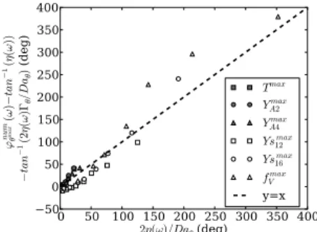
in Section 2.2, Fig. 5 presents the obtained numerical
phase lag due to this delay time as a function of the ex-7
pected one. This phase lag is obtained by substracting
to the obtained numerical phase lag 'num
✓max(!) the
theo-retical phase lag of the equivalent steady strain rate A✓
of the variable of interest ✓. Good results are obtained for all the species and temperature, which confirms the
representativity of the chosen variable (⌧✓).
Neverthe-less, some discrepancies exist and future investigations are still needed in order to define in a more precise way this delay time.
Figure 5. Numerical results of the induced phase lag due to the delay time imposed by slow chemistry as a function of the expected ones.
4.4. Numerical results at high amplitudes
In order to study the soot dynamics at higher am-plitudes, computations have been performed for
ampli-tudes ↵ of 30% and 60%. Table2 compares the
nu-merical results for the phase lag and amplitude gain of
Ymax
A4 and fVmax for three amplitudes and three
frequen-cies. The phase lag increases with the frequency in a similar way for all the amplitudes. The gain remains almost the same for ↵ = 10% and ↵ = 30%, but de-creases for ↵ = 60%. The di↵erence of the numerical behavior between ↵ = 30% and ↵ = 60% highlights the non-linear e↵ects for such amplitudes, which cannot be described by the linear analytical model whose predic-tions do not depend on the perturbation amplitude. 5. Conclusions
Response of sooting propane-air counterflow di↵u-sion flames to imposed strain rate harmonic oscillations were numerically investigated with a detailed descrip-tion for the gas and the solid phases. The unsteady be-havior of soot particles and precursors production, as well as the PSD evolution, were studied both analyt-ically and numeranalyt-ically. It has been observed that the higher the oscillation frequency is, the more PAHs and soot particles fluctuations are damped and phase-lagged so that unsteady solutions are farther and farther away
f ✓ ↵ =10% ↵ =30% ↵ =60%
(Hz) G✓max '✓max G✓max '✓max G✓max '✓max
30 A4 -4 54 -4 53 -5 56 30 fV -4 146 -4 158 -13 142 60 A4 -9 87 -8 91 -10 87 60 fV -14 269 -14 287 -24 256 120 A4 -16 126 -16 134 -18 130 120 fV -33 460 -33 524 -41 497
Table 2. Numerical analysis of the impact of the strain fluctuation am-plitude (↵) on the pyrene maximum mass fraction and soot maximum volume fraction gain (G in dB) and phase lag (' in deg).
from the quasi-steady state. The phase-lag and damping increase with the size of PAHs and soot particles.
An analytical model has been proposed to predict the observed phase lags and dampings assuming a linear
be-havior. Three non-dimensional parameters (⌘, Da✓and
✓) govern the unsteady response. Soot particles are
characterized by long time scales mainly due to conden-sation and coagulation phenomena. Indeed, compared to the gas species, their dynamics, particularly the addi-tional identified phase lag, are mainly governed by the
Da✓parameter.
Therefore, models developped for numerical simu-lations of soot production in turbulent flames have to correctly reproduce these observed features in order to represent unsteady behaviors such as soot intermittency. On the one hand, these behaviors highlight the limits of flamelet regime assumption based on quasi-steady hy-pothesis, implying major complexities in modeling for turbulent calculations. In this sense, the presented
re-sults support the need for specific techniques [31] to
ac-count for PAHs response to unsteady strain rate fluctu-ations. On the other hand, the reduced models have to
provide a good prediction of ⌘, Da✓ and ✓ for PAHs
and soot. As an example, representative soot precursors have to be chosen in terms of these three parameters in order to obtain the good unsteady behavior of soot pro-duction: large precursors dynamics (such as pyrene and coronen) have to be reproduced. The proposed analyt-ical model will be very useful for the development of models that reproduce the dynamics of soot and their precursors in turbulent flames.
AppendixA. Chemical characteristic time scales Species and flame characteristic time scales.
To study the unsteady response of each chemical
the kthspecies is defined as [32]:
⌧k=[Xk]max/˙!maxk =(⇢Yk)max/
⇣ Wk˙!maxk
⌘
(A.1)
where [Xk], Yk, Wkand ˙!kare the molar concentration,
the mass fraction, the molecular weight and the molar
production rate of the kthspecies.
In the same way, the characteristic time scale ⌧T of
the flame can be defined as ⌧T =⇣⇢cpT⌘max/˙!maxT , with
cp the mixture mass specific heat capacity and ˙!T the
heat release rate.
Soot sections characteristic time scales.
As for the species, a time scale ⌧s,ifor the soot
parti-cles in the ithsection can be defined as:
⌧s,i=(⇢Ys,i)max/⇣⇢s( ˙Qs,i)max⌘ (A.2)
By perturbing each volume fraction production rate relative to each phenomenon (ph) by a small value
(typ-ically 1%), the characteristic time scales ⌧nu,ifor
nucle-ation, ⌧cond,ifor condensation, ⌧sg,ifor surface growth,
⌧ox,ifor oxidation and ⌧coag,i for coagulation can be
ex-pressed as:
⌧ph,i= ⇥(⇢Ys,i/⇢s)max⇤/ h( ˙Qph,i)maxi (A.3)
where h( ˙Qph,i)max
i
corresponds to the variation of the peak volume fraction production rate of the
phe-nomenon for the ithsection.
References
[1] J. Quaas,Nature471 (7339) (2011) 456–457.
[2] M. D. Smooke, M. B. Long, B. C. Connelly, M. B. Colket, R. J. Hall,Combust. Flame143 (4) (2005) 613–628.
[3] P. Desgroux, X. Mercier, K. A. Thomson,Proc. Combust. Inst. 34 (1) (2013) 1713–1738.
[4] V. Raman, R. O. Fox,Annual Review of Fluid Mechanics(2015) 159–190.
[5] A. Attili, F. Bisetti, M. E. Mueller, H. Pitsch,Combust. Flame 161 (7) (2014) 1849–1865.
[6] Y. Xin, J. P. Gore,Proc. Combust. Inst.30 (1) (2005) 719–726. [7] B. Franzelli, P. Scouflaire, S. Candel,Proc. Combust. Inst.35 (2)
(2015) 1921–1929.
[8] N. Peters,Prog. Energy Combust. Sci.10 (3) (1984) 319–339. [9] D. Veynante, L. Vervisch,Prog. Energy Combust. Sci.28 (3)
(2002) 193–266.
[10] B. Cuenot, F. Egolfopoulos, T. Poinsot,Combust. Theor. Model. 4 (1) (2000) 77–97.
[11] D. C. Haworth, M. C. Drake, S. B. Pope, R. J. Blint,Symposium
(International) on Combustion22 (1) (1989) 589–597.
[12] S. Candel,Proc. Combust. Inst.29 (1) (2002) 1–28.
[13] M. E. Decroix, W. L. Roberts,Combust. Sci. Technol.160 (1) (2000) 165–189.
[14] D. Santoianni, M. DeCroix, W. Roberts,Flow Turbul. Combust. 66 (1) (2001) 23–36.
[15] J. Xiao, E. Austin, W. L. Roberts, Combust. Sci. Technol. 177 (4) (2005) 691–713.
[16] A. Cuoci, A. Frassoldati, T. Faravelli, E. Ranzi,Combust. Flame 156 (10) (2009) 2010–2022.
[17] V. Huijnen, A. V. Evlampiev, L. M. T. Somers, R. S. G. Baert, L. P. H. de Goey,Combust. Sci. Technol.182 (2) (2010) 103– 123.
[18] B. V. Derjaguin, A. I. Storozhilova, Y. I. Rabinovich,J. Colloid
Interface Sci.21 (1) (1966) 35–58.
[19] P. S. Epstein,Phys. Rev.23 (1924) 710–733.
[20] D. Aubagnac-Karkar, J.-B. Michel, O. Colin, P. E. Vervisch-Kljakic, N. Darabiha,Combust. Flame162 (8) (2015) 3081– 3099.
[21] M. Mueller, G. Blanquart, H. Pitsch,Combust. Flame156 (6) (2009) 1143 – 1155.
[22] Y. Wang, A. Raj, S. H. Chung,Combust. Flame160 (9) (2013) 1667 – 1676.
[23] F. Mauss, T. Schäfer, H. Bockhorn,Combust. Flame99 (3–4) (1994) 697 – 705, 25th Symposium (International) on Combus-tion Papers.
[24] F. Xu, A. M. El-Leathy, C. H. Kim, G. M. Faeth, Combust.
Flame132 (1–2) (2003) 43–57.
[25] M. Smoluchowski, Versuch einer mathematischen Theorie der Koagulationskinetik kolloider Lösungen, 1916.
[26] A. Soufiani, J. Taine,Int. J. Heat Mass Transfer40 (4) (1997) 987–991.
[27] L. Tessé, F. Dupoirieux, J. Taine, Int. J. Heat Mass Transfer 47 (3) (2004) 555–572.
[28] N. Darabiha, N.,Combust. Sci. Technol.86 (1-6) (1992) 163– 181.
[29] B. Franzelli, B. Fiorina, N. Darabiha,Proc. Combust. Inst.34 (1) (2013) 1659–1666.
[30] C. Saggese, S. Ferrario, J. Camacho, A. Cuoci, A. Frassoldati, E. Ranzi, H. Wang, T. Faravelli,Combust. Flame162 (9) (2015) 3356–3369.
[31] Y. Xuan, G. Blanquart,Proc. Combust. Inst.35 (2) (2015) 1911– 1919.
[32] H. G. IM, J. H. Chen, J.-Y. Chen,Combust. Flame118 (1–2) (1999) 204–212.