HAL Id: hal-01562449
https://hal.inria.fr/hal-01562449
Submitted on 14 Jul 2017
HAL is a multi-disciplinary open access
archive for the deposit and dissemination of
sci-entific research documents, whether they are
pub-lished or not. The documents may come from
teaching and research institutions in France or
L’archive ouverte pluridisciplinaire HAL, est
destinée au dépôt et à la diffusion de documents
scientifiques de niveau recherche, publiés ou non,
émanant des établissements d’enseignement et de
recherche français ou étrangers, des laboratoires
Fiberprint: A subject fingerprint based on sparse code
pooling for white matter fiber analysis
Kuldeep Kumar, Christian Desrosiers, Kaleem Siddiqi, Olivier Colliot,
Matthew Toews
To cite this version:
Kuldeep Kumar, Christian Desrosiers, Kaleem Siddiqi, Olivier Colliot, Matthew Toews. Fiberprint: A
subject fingerprint based on sparse code pooling for white matter fiber analysis. NeuroImage, Elsevier,
2017, 158, pp.242 - 259. �10.1016/j.neuroimage.2017.06.083�. �hal-01562449�
Fiberprint: a subject fingerprint based on sparse code
pooling for white matter fiber analysis
Kuldeep Kumara,∗1, Christian Desrosiersa, Kaleem Siddiqib,
Olivier Colliotc,d,e, Matthew Toewsa
aLaboratory for Imagery, Vision and Artificial Intelligence, ´Ecole de technologie sup´erieure,
1100 Notre-Dame W., Montreal, QC, Canada, H3C1K3
bSchool of Computer Science & Center for Intelligent Machines, McGill University,
3480 University Street, Montreal, QC, Canada, H3A2A7
cSorbonne Universit´es, UPMC Univ Paris 06, Inserm, CNRS, Institut du cerveau et la
moelle (ICM) - Hˆopital Piti´e-Salpˆetri`ere, Boulevard de l′hˆopital, F-75013, Paris, France dInria Paris, Aramis project-team, 75013, Paris, France
eAP-HP, Departments of Neurology and Neuroradiology, Hˆopital Piti´e-Salpˆetri`ere, 75013,
Paris, France
Abstract
White matter characterization studies use the information provided by diffu-sion magnetic resonance imaging (dMRI) to draw cross-population inferences. However, the structure, function, and white matter geometry vary across indi-viduals. Here, we propose a subject fingerprint, called Fiberprint, to quantify the individual uniqueness in white matter geometry using fiber trajectories. We learn a sparse coding representation for fiber trajectories by mapping them to a common space defined by a dictionary. A subject fingerprint is then gener-ated by applying a pooling function for each bundle, thus providing a vector of bundle-wise features describing a particular subject’s white matter geometry. These features encode unique properties of fiber trajectories, such as their den-sity along prominent bundles. An analysis of data from 861 Human Connectome Project subjects reveals that a fingerprint based on approximately 3 000 fiber trajectories can uniquely identify exemplars from the same individual. We also use fingerprints for twin/sibling identification, our observations consistent with the twin data studies of white matter integrity. Our results demonstrate that the proposed Fiberprint can effectively capture the variability in white matter
fiber geometry across individuals, using a compact feature vector (dimension of 50), making this framework particularly attractive for handling large datasets. Keywords: Subject fingerprint, dMRI, White matter geometry, fiber
trajectories, Sparse Code Pooling, HCP, Twin data
1. Introduction
Diffusion magnetic resonance imaging (dMRI) is a powerful and non-invasive tool that provides key information on white matter organization and connectiv-ity based on the diffusion of water molecules in white matter tissues [1]. Recent advances in dMRI acquisition protocols have lead to significant improvements
5
in signal reconstruction [2, 3, 4], driving the development of novel tools for pro-cessing and interpreting dMRI data. Among the many applications using dMRI data, the quantitative characterization of white matter geometry and its genetic basis [5, 6, 7] is an important step in the study of the human brain, essential to understanding the mechanisms of neurological function and disease [8, 9, 10, 11].
10
Over the years, several approaches have been proposed to provide a sim-plified quantitative description of white matter connections, to allow for cross-population inferences [12, 13, 14, 15]. While numerous studies have focused on elucidating brain connectivity patterns that are shared across people, re-searchers have also acknowledged the high individual variability in brain
struc-15
ture [16, 17, 18], function [19, 20, 21, 22, 23, 24], and white matter geometry [25, 26]. Motivated by this, the concept of connectome fingerprinting, which characterizes individuals using unique connectivity profiles, has recently drawn significant interest from the neuroscience community [27, 28, 29, 30, 31, 32, 33]. So far, most studies on subject fingerprinting have centered around
func-20
tional [27, 28, 29] and structural data [31, 34]. Recently, a novel approach was proposed for building individual connectome profiles based on dMRI data [33, 35]. This approach uses the Spin Distribution Function (SDF) at each voxel to obtain a fingerprint encoding the diffusion density along a set of prominent directions in cerebral white matter. While it captures key characteristics of
white matter diffusivity, this voxel-level fingerprint lacks direct correspondence with white matter bundles, thus hindering an intuitive representation and anal-ysis. As highlighted in [36], a direct voxelwise comparison of diffusion imaging data could also be challenging, since the high-contrast edges in diffusion MRI volumes (e.g., FA maps) make them more susceptible to small registration
er-30
rors. Such comparison is also complicated by the anatomical variability of tract positions in subjects.
Building a fingerprint at the level of fiber trajectories, instead of voxels, could provide a more meaningful way of analyzing the unique connectivity properties of individuals from dMRI data. However, working with fiber trajectories also
35
presents additional difficulties, due to the fact that the number and distribu-tion of fiber trajectories may vary across subjects, and fiber trajectories may have very different lengths. Finding a common representation space of fiber trajectories, in different subjects, is essential to overcome these difficulties.
In recent work, we introduced a framework based on sparse coding for the
40
compact representation and cross-population analysis of fiber trajectories [37]. This framework utilizes dictionary learning to build an atlas of fiber bundles from multi-subject dMRI data. Via sparse coding, this atlas can then be used to encode new fiber trajectory data into a compact representation, common to all subjects, and segment these fiber trajectories into prominent bundles [38].
45
In the current paper, we propose to use this framework to characterize the uniqueness in white matter connectivity exhibited by individual subjects, at the level of fiber trajectories. The key idea of our work is to represent each fiber trajectory as a sparse weighted combination of atlas bundles (i.e., the dictionary atoms), and use a pooling function [39] to combine the sparse codes of a subject’s
50
fiber trajectories into a single feature vector representing bundle-wise properties of fiber trajectory geometry. The resulting fingerprint, called Fiberprint, is used to uniquely identify subjects, as well as to discover inheritable characteristics of fiber geometry by comparing the fingerprints of twins and non-twin siblings. The use of fiber trajectories as a basis for the proposed subject fingerprint is
55
of fiber bundles varies across subjects. However, characterizing an individual subject’s white matter fiber geometry via a signature has thus far been elusive. The main contribution of our work is the use of sparse code pooling to build a subject fingerprint, called Fiberprint. To our knowledge, this is the first study
60
to propose a fingerprint based on fiber geometry. Another notable contribution of this work is the large-scale analysis and validation of our fingerprint, involving a cohort of 861 subjects from Human Connectome Project.
The rest of this paper is organized as follows. We first give an overview of related work on brain fiber analysis, sparse coding, and subject
fingerprint-65
ing. Section 3 then presents the proposed Fiberprint approach, based on non-negative kernel sparse coding. In Section 4, we conduct an extensive experimen-tal validation using the dMRI data of 861 subjects from the Human Connectome Project dataset, in which the impact of various parameters of our approach is measured. We also evaluate the usefulness of the proposed fingerprint on the
70
task of subject, twin, and non-twin sibling identification, and use hypothesis testing to find bundles showing significant fingerprint dissimilarities across dif-ferent subjects groups (i.e., males vs females). In Section 5, we discuss our main observations and experimental findings. We conclude with a summary of our contributions and a discussion of possible extensions.
75
2. Related work
Our presentation of relevant work is divided into three parts, focusing re-spectively on the representation and analysis of white matter fiber geometry, the application of sparse coding techniques in neuroimaging, and the topic of subject fingerprinting.
80
2.1. Representation and analysis of white matter fiber geometry
White matter fiber characterization often assumes an initial abstraction based on tractography, where local diffusion information is used to recover streamlines representing connectivity pathways in the brain [40, 41, 42]. Since
tractography may output thousands of fiber trajectories, early work has
fo-85
cused on finding simplified quantitative descriptions of white matter connec-tions by grouping fiber trajectories into anatomically meaningful bundles [43]. Over the years, a wide range of approaches have been proposed to cluster fiber trajectories, including methods based on hierarchical clustering [44, 45] and spectral clustering [46, 47, 48]. Most of these methods group fiber trajectories
90
using problem-specific measures of similarity, such as the Hausdorff distance [44, 45, 49] or a mean of closest points (MCP) distance [44, 50, 45, 49].
Various studies have also focused on the segmentation of white matter tracts, toward the goal of drawing cross-population inferences [12, 13, 14, 15]. These studies either follow an atlas based approach [12, 13, 14] or align specific tracts
95
directly across subjects [51, 52]. Multi-step or multi-level approaches have also been proposed to segment fiber trajectories, for example, by combining both voxel and fiber trajectory groupings [12], fusing labels from multiple hand-labeled atlases [13], using a white matter voxel-space atlas and a bundle rep-resentation based on maximum density paths [15], or using Gaussian processes
100
[53]. A few studies have also investigated the representation of specific fiber tra-jectory bundles using different techniques such as gamma mixture models [54], hierarchical Dirichlet processes [55], and the computational model of rectifiable currents [56, 57].
2.2. Sparse coding for neuroimaging
105
Sparse coding, which aims at encoding a signal as a sparse combination of prototypes in a data-driven dictionary, has been applied in various domains of computer vision and pattern recognition [58, 59, 60, 39]. This technique has also shown promise for various neuroimaging applications, such as the recon-struction [61] or segmentation [62] of MRI data, and for functional connectivity
110
analysis [63, 64]. For diffusion data, sparse coding has been used successfully for clustering white matter voxels from Orientation Density Function (ODF) data [65], and for finding a population-level dictionary of key white matter tracts [66].
To deal with the challenges of anatomic and tractographic variability, we
115
have recently proposed a framework based on non-negative kernel dictionary learning for grouping fiber trajectories into prominent bundles [37]. This frame-work encodes individual fiber trajectories as a sparse non-negative combination of dictionary prototypes corresponding to bundles. Unlike other fiber trajectory clustering approaches, which assign fiber trajectories to individual bundles, the
120
proposed framework gives fiber trajectories a membership value to each bundle, thus providing a more intuitive way of dealing with overlapping bundles and inter-subject variability. In a later study, the same framework was used to learn a multi-subject atlas of fiber bundles and for the automatic segmentation of new fiber trajectory data [38].
125
2.3. Subject fingerprinting
Most neuroimaging studies collapse multi-subject data to draw inferences about common patterns in a population. Although there are gross similarities, a substantial portion of a subject’s connectome is unique to that individual [19, 25, 20, 17, 21, 18, 22]. A recent study has shown that functional connectivity profiles
130
act as robust and reliable fingerprints that can identify individual subjects from a large group [28]. In this study, a functional brain atlas was employed to define target brain regions. The Pearson correlation coefficients between the time courses of region pairs were then computed, and used as a functional connectivity profile. This fingerprint was able to identify individuals across
135
scan sessions, both for task and rest conditions.
In [31], Wachinger et al. proposed Brainprint, a subject fingerprint that characterizes brain morphology by calculating the spectrum of the Laplace-Beltrami operator on meshes from cortical and subcortical brain structures. This fingerprint was used to study morphological similarity between brains,
140
with applications in subject identification across multiple scans of the same subject (achieving a classification accuracy of up to 99.9%), and the analysis of potential genetic influences on brain morphology.
structural data, a local connectome fingerprint using Spin Distribution Function
145
(SDF) voxel profiles obtained from dMRI data has recently been proposed in [32, 35]. This local fingerprint is built by sampling, at each voxel, the diffusion density of water along principal directions in the white matter, defined using a common fiber-direction atlas. The proposed fingerprint was used for quantifying the similarity between genetically-associated individuals, as well as measuring
150
neuroplasticity over time, and was shown to vary substantially across individual subjects compared to traditional diffusivity measures like Fractional Anisotropy (FA). However, since this fingerprint is built using voxel-level information, it lacks a direct correspondence with white matter bundles, and a direct voxel-level comparison of diffusion imaging data could be challenging, as the high-contrast
155
edges of diffusion MRI volumes (e.g., FA maps) make them more susceptible to small misregistration errors, as well as to anatomical variability of tract positions in health and disease [36]. Another point is that this fingerprint tries to capture both voxel-level diffusivity information and morphology. To our knowledge, the present study is the first to propose a white matter geometry fingerprint at the
160
level of fiber trajectories and fiber bundles.
3. Materials and methods
1. Fiber tracking 2. Dictionary learning 3. Fiber encoding 4. Pooling 5. Subject identification /Bundle significance Tractogram
(MNI space)
Bundle dictionary
Sparse codes Sparse codes
Subject Fingerprint Fiberprint
dMRI data
(861 subjects)
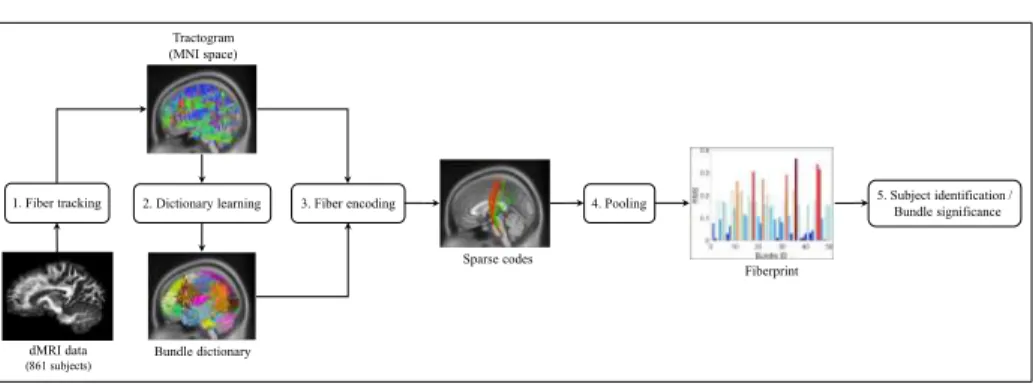
Figure 1: Pipeline of the proposed Fiberprint approach based on sparse code pooling.
Figure 1 summarizes the pipeline of the proposed Fiberprint method, com-prised of three steps. In the first step, signal reconstruction and fiber tracking
is performed on the pre-processed dMRI data of 861 subjects from the Human
165
Connectome Project [67, 68]. Second, a dictionary of prototype fiber trajecto-ries is then learned from a subset of subjects, based on our non-negative kernel dictionary learning framework. This dictionary can be seen as an atlas for mod-eling and analyzing the geometry of fiber trajectories from multiple subjects, along prominent bundles. In the third step, the learned dictionary is used to
en-170
code the fiber trajectories of the remaining subjects in a common feature space, via a sparse coding method. A fingerprint is then obtained, for each subject, by applying a pooling function to the sparse codes corresponding to each sub-ject’s fiber trajectories. This pooling function allows the comparison of subjects having a different number of fiber trajectories by aggregating the information
175
from all fiber trajectories in a single fixed-size vector. The resulting fingerprint corresponds to an estimate of fiber trajectory density along key bundles defined by the atlas. Finally, in the last step, fingerprints are used to identify unique characteristics of genetically-related subjects, or for finding bundles showing significant differences across various subject groups (e.g., male vs female). The
180
following subsections describe each of these steps in greater detail. 3.1. Data and pre-processing
We used the pre-processed dMRI data of 861 subjects (482 females, 378 male and 1 unknown, age 22–35) from the Q3 release of the Human Connectome Project [69, 67, 68], henceforth referred to as HCP data. All HCP data measure
185
diffusivity along 270 directions distributed equally over 3 shells with b-values of
1000, 2000 and 3000s/mm2, and were acquired on a Siemens Skyra 3T scanner
with the following parameters: sequence = Spin-echo EPI; repetition time (TR)
= 5520 ms; echo time (TE) = 89.5 ms; resolution = 1.25× 1.25 × 1.25 mm3
voxels. Further details can be obtained from HCP Q3 data release manual2.
190
For signal reconstruction and tractography, we used the freely available DSI Studio toolbox. All subjects were reconstructed in MNI space using the Q-space
diffeomorphic reconstruction (QSDR) [70] option in DSI Studio. QSDR is an extension of generalized q-sampling imaging (GQI, [71]), allowing the construc-tion of spin distribuconstruc-tion funcconstruc-tions (SDF) in a given template space. DSI Studio
195
first calculates the quantitative anisotropy (QA) mapping in the native space and then normalizes it to the MNI QA map using SPM normalization [72]. We used the SPM 21-27-21 option in DSI Studio for normalization, and set output resolution to 1 mm. For skull stripping, we used the masks provided with pre-processed diffusion HCP data. Other parameters were set to the default DSI
200
Studio values. We also normalized T1-weighted images to MNI template space as part of this processing.
Deterministic tractography was performed with the Runge-Kutta method of DSI Studio [40, 73], using the following parameters: minimum length of 40 mm, turning angle criteria of 60 degrees, and trlinear interpolation. The termination
205
criteria was based on the QA value, which is determined automatically by DSI Studio. As in the reconstruction step, the other parameters were set to the default DSI Studio values. Using this technique, we obtained a total of 50 000 fiber trajectories for each subject.
As a note, whether these fiber trajectories represent the actual white matter
210
pathways remains a topic of debate [74, 75]. Fiber trajectories derived from DSI studio are hypothetical curves in space that represent, at best, the major axonal directions suggested by the orientation distribution functions of each voxel, which may contain tens of thousands of actual axonal fibers.
3.2. Learning the fiber trajectory dictionary
215
Out of the 861 available subjects, 10 unrelated ones [76] were used to learn the dictionary of fiber trajectory prototypes, serving as a multi-subject atlas to map new fiber trajectory data to a common space. The learning process is based on the non-negative kernel dictionary learning method presented in [37, 38], which we now summarize.
220
Let X be the set of n training fiber trajectories, represented as a set of 3D coordinates. For the purpose of explanation, we suppose that each trajectory i
is encoded as a feature vector xi ∈ Rd, and that X is a d× n feature matrix.
Since our dictionary learning method is based on kernels, a fixed set of features is however not required, and fiber trajectories having a different number of
225
3D coordinates could be compared with a suitable similarity measure (i.e., the kernel function).
In the proposed model, each fiber trajectory can be described as a sparse linear combination of m prototype fiber trajectories in a dictionary D. Formally,
we write this as xi ∼ Dwi, where wi is a sparse vector of non-negative weights
230
representing the fiber trajectory’s relationship to each prototype. Since fiber trajectories may have very different lengths and endpoints, encoding them using a fixed set of features can be challenging. To avoid this problem, we embed
them into a q-dimensional Hilbert space via a mapping function φ :Rd → Rq,
such that φ(x)⊤φ(x′) = k(x, x′) is a kernel function. The main advantage
235
of this approach is that fiber trajectories can now be represented based on a similarity measure tailored to this type of data, such as the Hausdorff distance [44, 45, 49], the mean of closest points (MCP) distance [44, 50, 45, 49] or the Minimum average Direct Flip (MDF) distance [77]. In this work, we considered the MDF distance, which computes the average distance between points on a
240
fiber trajectory and corresponding points in a second fiber trajectory, or in the reverse point sequence of the second fiber trajectory if it leads to a smaller distance. A Gaussian kernel was used to convert distances to similarities, i.e.
k(x, x′) = exp!− γ · distMDF(x, x′)". The fiber trajectories were sampled to
15 equidistant points for distance computation [77] and the kernel bandwidth
245
parameter was set empirically to γ = 0.0001.
Using Φ∈ Rq×nto denote the matrix of mapped training fiber trajectories,
the kernel matrix of pairwise similarities then corresponds to K = Φ⊤Φ. Using
the idea proposed in [78], we express the dictionary as a non-negative linear
combination of training examples, i.e., D∼ ΦA, and formulate the dictionary
learning task as the following optimization problem: arg min A, W≥ 0 1 2∥Φ − ΦAW ∥ 2 F s.t. ∥wi∥0≤ Smax, i = 1, . . . , n, (1)
where ∥wi∥0 is the L0 norm (i.e., number of non-zero elements) of wi,
con-straining each fiber trajectory to be encoded using at most Smax prototypes,
A∈ Rn×mis the dictionary coefficient matrix, and W∈ Rm×nis the sparse code
matrix for all fiber trajectories. When Smax= 1, this formulation corresponds
250
to the kernel K-means problem [79]. As shown in Section 4.1.4, expressing fiber
trajectories using more than one prototype (i.e., Smax > 1) provides a better
representation of complex bundles, leading to a more discriminative fingerprint. This problem is solved using the method described in [37], which updates the sparse codes W and dictionary matrix A iteratively, until convergence. In the sparse coding step, each column of W is updated independently by optimizing the following sub-problem:
arg min wi≥ 0 1 2w ⊤ i A⊤KAwi − ki⊤Awi s.t. ∥wi∥0≤ Smax, (2)
where ki∈ Rn is the vector containing the similarities between fiber trajectory
i and all training fiber trajectories. This problem is solved heuristically using a non-negative kernel Orthogonal Matching Pursuit (NKOMP) algorithm [37]. The dictionary matrix A is then obtained using a kernel version of the non-negative matrix tri-factorization approach proposed in [80], which applies the following update scheme until convergence:
Aij ← Aij· ! KW⊤" ij (KAW W⊤) ij , ∀ i, j. (3)
Due to machine precision, the above update scheme produces small positive values instead of zero entries. To resolve this problem, a small threshold is
255
applied on A.
Since the kernel contains the similarities between each pair of fiber
trajecto-ries (50 000×10 fiber trajectories, squared), computing it directly is
impractica-ble. Instead, we start with 5 000 fiber trajectories sampled uniformly from each
subject, and approximate the resulting kernel matrix (50 000× 50 000) using
260
Nystrom’s method [81, 14]. This method starts with defining a subset of fiber trajectories and computing the pairwise similarities between each training fiber trajectory and this sampled subset. The missing entries in kernel matrix K are
then estimated using a low-rank approximation process based on SVD. Using this technique, the entire dictionary learning process takes about 1 000 seconds
265
on a quad-core 3.6 GHz computer with 32 GB of RAM.
Figure 1: Dictionary visualization. Visualization of m = 50 fiber prototypes learned from 10 subjects, with an unique color assigned to each dictionary prototype. For this simplified visualization each fiber is assigned to a single prototype by taking the maximum for each row of the matrix A. (superior axial, left sagittal, and anterior coronal views respectively) Figure 2: Dictionary visualization. Visualization of m = 50 fiber trajectory prototypes learned from 10 subjects, with an unique color assigned to each dictionary prototype. For this simpli-fied visualization each fiber trajectory is assigned to a single prototype by taking the maximum for each row of the matrix A. (superior axial, left sagittal, and anterior coronal views respec-tively)
Figure 2 gives a qualitative visualization of m = 50 fiber trajectory proto-types learned in the dictionary (the impact of parameter m is analyzed in Section 4.1.2), each one corresponding to a different color. To generate this figure, we convert the soft assignment defined in A to a hard clustering, by assigning each
270
fiber trajectory i to the prototype j for which aij is maximum3. We see that
the fiber trajectory clusters defined by the dictionary are reasonably consistent with prominent neuroanatomical bundles, such as the corpus callosum, cingu-lum, corticospinal tract and superior cerebellar penduncle. Note, however, that a one-to-one relationship does not always hold between these prototypes and
275
neuroanatomical bundles: complex bundles may be represented using multiple prototypes. Nonetheless, to simplify the presentation, we use the term bundle dictionary when referring to the output of the dictionary learning step.
3A separate visualization of each fiber trajectory cluster can be found in the supplementary
material.
3.3. Generating the subject fingerprints
The generation of a fingerprint from the fiber trajectory data of a new subject
280
is composed of two steps: sparse coding of fiber trajectories and sparse code pooling.
Sparse coding of fiber trajectories
In the first step, the learned dictionary is used to map the fiber trajectories of a given subject to a common feature space defined by the dictionary’s
bun-285
dles. This encoding process consists of solving the sparse coding problem of Eq. (2), which has been used for dictionary learning. Since each fiber trajectory is
represented using at most Smax coefficients, this re-encoding of a subject’s fiber
trajectory data is very compact.
The fiber trajectory sparse codes of four different subjects, obtained using
290
the dictionary of Figure 2, are illustrated in Figure 3. We represent bundles using the same colors as in Figure 2, and assign each fiber trajectory i to the
bundle for which wji is maximum, where W is the sparse code matrix of a
given subject. This hard assignment of fiber trajectories to dictionary bundles corresponds to the fiber trajectory segmentation approach presented in [38]. The
295
strength of the relationship between fiber trajectories and individual bundles can also be visualized by considering the values in each row of W . In Figure 4, the sparse code values (i.e., rows of W ) corresponding to the left and right corticospinal bundles are color coded such that fiber trajectories having a high membership to a bundle are red and those having a low membership are green
300
(fiber trajectories with zero membership are not shown). These figures highlight the implicit correspondence of bundles across subjects, as well as the variability in the fiber trajectory geometry of bundles, observed for different subjects. Sparse code pooling
Because subjects may have a different number of fiber trajectories, to allow
305
comparison across subjects, the sparse codes for fiber trajectories obtained in the previous step must be aggregated in a fixed-size feature vector. This is
Subject 1 Subject 2 Subject 3 Subject 4
Figure 1: Visualization of sparse code representation of fibers from four subjects. Each fiber is assigned to a single bundle by taking the maximum of the sparse code vector. Bundles are represented using the same colors as in Figure ??. (superior axial (top), left sagittal (middle), and anterior coronal (bottom) views respectively)
Figure 3: Visualization of sparse code representation of fiber trajectories from four subjects. Each fiber trajectory is assigned to a single bundle by taking the maximum of the sparse code vector. Bundles are represented using the same colors as in Figure 2. (superior axial (top), left sagittal (middle), and anterior coronal (bottom) views respectively)
achieved using a sparse code pooling function [39] that combines, for each dic-tionary bundle, the relationship between this bundle and all fiber trajectories of
a subject into a single value. Let W ∈ Rm×nbe the sparse code matrix obtained
310
in the previous step, each column corresponding to a different fiber trajectory of the subject to encode. We consider three pooling functions frequently used in the literature, based on the root mean square (RMS), mean and maximum:
# fRMS(W )$j = % & & ' 1 n n ( i=1 w2 ji (4) # fMean(W ) $ j = 1 n n ( i=1 |wji| (5) # fMax(W )$j = max)|wj1|, |wj2|, . . . , |wjn|*. (6)
Subject 1 Subject 2 Subject 3 Subject 4
Figure 1: Color coded visualization of sparse code memberships of fibers for the left (top row) and right (bottom row) corticospinal bundles from four subjects. Green and red represent, a low and a high membership of a fiber to a bundle, respectively. Fibers with a zero membership to the bundle are removed for a simplified visualization.
Figure 4: Color coded visualization of sparse code memberships of fiber trajectories for the left (top row) and right (bottom row) corticospinal bundles from four subjects. Green and red represent, a low and a high membership of a fiber trajectory to a bundle, respectively. Fiber trajectories with a zero membership to the bundle are removed for a simplified visualization.
where [f (W )]j is the pooled feature corresponding to the j-th dictionary
bundle.
315
Each of these pooling functions encodes a different property of a subject’s
fiber trajectory distribution along the dictionary bundles. Function fmean
com-putes the average sparse code value of fiber trajectories belonging to a bundle,
thus giving an estimate of the bundle’s density. fRMS is another measure of
density, which gives a greater importance to large magnitude values in W .
Fi-320
nally, fmax selects the maximum sparse code value over all fiber trajectories in
relationship to a given bundle. In practice, this value will be low for dictionary prototypes which are not useful for encoding a subject’s fiber trajectories.
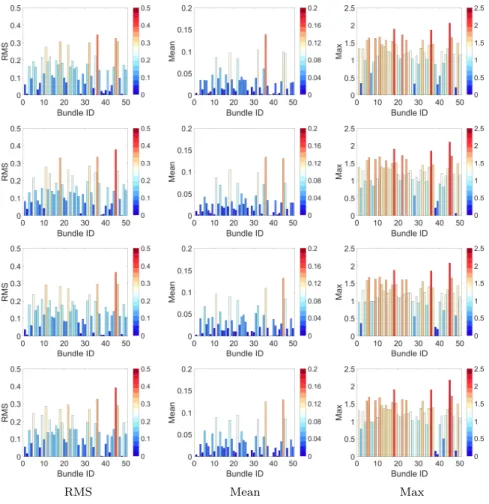
Figure 5 shows a bar plot representation of fingerprints obtained using the three pooling functions, for four different subjects. We observe small but
mean-325
ingful differences when comparing these fingerprints, supporting the hypothesis that they encode unique characteristics of fiber trajectory geometry. Moreover, we see that the pooling functions capture different properties (in particular the max pooling function) and have varying responses across bundles. The unique-ness of subject fingerprints can be further visualized in Figure 6, which color
codes the fiber trajectory bundles of the four subjects based on the magnitude of their corresponding RMS pooling function values. We observe that the bun-dles showing the highest response are consistent across subjects, although the magnitude of these responses differs from one subject to another.
RMS Mean Max
Figure 5: Subject fingerprint visualization. Color coded bar plot representation for four subjects (rows) and three pooling functions (RMS, Mean, and Max; columns), plotted as a value per bundle ID.
4. Experiments and results
335
In this section, we test the hypothesis that the proposed subject finger-print can effectively capture a particular subject’s white matter fiber geometry.
Subject 1 Subject 2 Subject 3 Subject 4
Figure 1: Subject fingerprint visualization. Color coded bundles from four subjects repre-senting the magnitude of their corresponding RMS pooling function values. We use the same color code scheme as in Figure ??. (superior axial (top), left sagittal (middle), and anterior coronal (bottom) views respectively)
Figure 6: Subject fingerprint visualization. Color coded bundles from four subjects repre-senting the magnitude of their corresponding RMS pooling function values. We use the same color code scheme as in Figure 5. (superior axial (top), left sagittal (middle), and anterior coronal (bottom) views respectively)
Because there are many parameters and factors involved in the generation of fin-gerprints (e.g., pooling function, dictionary size, and fiber tracking approach), we first perform an analysis to assess the robustness of our fingerprint to these
340
various parameters and factors. We then validate our main hypothesis using the task of subject identification and twin identification. Specifically, we try to determine if an individual can be identified using the proposed fingerprint, and whether this fingerprint can discriminate between twin and non-twin siblings. In the process, we also analyze important properties of our fingerprint, such
345
hemi-spheres, required to characterize a subject’s fiber trajectory geometry. Finally, we conduct a significance testing analysis to identify fiber trajectory bundles which show important differences related to the genetic proximity of siblings (i.e., twins vs non-twins), and subject gender (i.e., males vs females).
350
4.1. Impact of method parameters
We first analyze the impact of various parameters on the proposed subject fingerprint’s ability to discriminate between subjects. The following parame-ters are considered in our analysis: the pooling function (i.e., RMS, Mean or Max), the dictionary size (i.e., m), the sets of dictionary learning subjects, the
355
fiber trajectory representation sparsity (i.e., Smax), the inclusion/exclusion of
cerebellar white matter, the fiber tracking parameters, and the number of fiber trajectories used to generate the fingerprint.
The fingerprint’s discriminability is measured quantitatively as follows. First, the 50 000 fiber trajectories of each subject (i.e., the 851 subjects not used for training the dictionary) are randomly divided into 5 instances, each one con-taining 10 000 fiber trajectories. These instances are then converted to subject fingerprints using the sparse coding and pooling process of Section 3.3, giving a
total of 851× 5 = 4 255 fingerprints. Each of these fingerprints is a vector of m
features, one for each dictionary bundle. We use the Euclidean distance between two fingerprints to measure their similarity, and evaluate the separability of the proposed approach by comparing the distribution of distances between same-subject instances and instances obtained from different same-subjects. The d-prime sensitivity index [82] is used to obtain a quantitative measure of separability:
d-prime = + µ1− µ2 1 2 ! σ2 1 + σ22 " , (7)
where, µ1, µ2are the means and σ1, σ2the standard deviations of the compared
distributions. Higher d-prime values indicate better separability. In this work
360
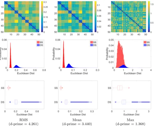
RMS (d-prime = 4.261) Mean (d-prime = 3.440) Max (d-prime = 1.368) Figure 7: Impact of pooling functions. Euclidean distance between fingerprints of 10 subjects with 5 instances each (top). Probability normalized histogram (middle) and box plot (bot-tom) for distances between same subject (SS) and different subject (DS) instances for all 851 subjects. Pooling functions: RMS, Mean, and Max (left to right columns respectively)
4.1.1. Pooling function
The impact of the pooling function on the fingerprint’s ability to distinguish subjects is analyzed in Figure 7. The top row of this figure shows the Euclidean distance between all pairs of instances from 10 different subjects, where
same-365
subject instances are grouped together. Except for the Max function, we
ob-serve a clear pattern where distances between same-subject instances (i.e., 5× 5
diagonal blocks) are smaller compared to distances between different-subject instances (off diagonal block elements). Pooling functions are further compared in the middle and bottom rows of the figure, showing the normalized histogram
370
computed for all 851 subjects. Once again, we notice a clear separation for the RMS and Mean pooling functions (d-prime of 4.261 and 3.440), but not the Max function (d-prime of 1.368). In an unpaired t-test, the means of same-subject and different-subject distances are significantly different, with p < 0.01.
375
Overall, this analysis shows that fingerprints obtained using the RMS and Mean pooling functions are significantly more similar for same-subject instances than instances from different subjects, and that the RMS function slightly out-performs Mean. As mentioned above, both functions estimate the fiber trajec-tory density along prominent bundles defined by the dictionary. In contrast,
380
the Max function leads to a poorly discriminative fingerprint. This could be due to the fact that features corresponding to each bundle are estimated us-ing a sus-ingle fiber trajectory with maximum sparse code magnitude, which does not capture the full variability in bundle geometry across subjects. The RMS pooling function was used for the remaining experiments of this study.
385
4.1.2. Dictionary size
The size of the dictionary (i.e., parameter m), which reflects the number of different bundles that can be captured by the encoding, can also impact the quality of the fingerprint: a small number of bundles may be insufficient to capture subtle differences between subjects, while having a large number of
390
bundles can affect the performance of the dictionary learning and sparse coding steps.
We tested seven different dictionary sizes, i.e. m = 10, 25, 50, 75, 100, 125, 150, while keeping the number of fiber trajectories per subject to 50 000. Note that varying m affects the number of fiber trajectories per bundle, as well as the
395
number of features in subject fingerprints. Figure 8 (left) shows the box plot of Euclidean distances between same-subject (red) and different-subject (blue) in-stances, for the tested dictionary sizes. We observe that the separation between same-subject and different-subject distance distributions increases slightly with the number of bundles, mostly due to a decrease in variance for distances
be-400
d-prime d-prime
Figure 8: Impact of the size of the dictionary and the level of sparsity Smax on subject
fingerprint. Box plot of Euclidean distances between same-subject (red) and different-subject (blue) instances for seven different dictionary sizes using all 851 subjects (left); and for varying level of the sparsity parameter Smaxusing 10 subjects (right).
fingerprint remains significant for dictionaries sizes of m ≥ 50, and using a
higher number of bundles may improve the consistency of the fingerprint. A dictionary size of m = 50 was used for the remaining experiments.
4.1.3. Independent dictionary sets
405
Since white matter geometry varies across individuals, changing the subjects used for learning the dictionary can also impact our fingerprint. To measure this impact, we created 5 different dictionaries learned from independent sets of 10 subjects, while keeping the sampling strategy and other parameters to their default values (m = 50). Figure 9 (top left) shows the box plot of Euclidean
dis-410
tances between same-subject and different-subject instances using each of these dictionaries. We observe no significant difference across dictionaries, demon-strating the robustness of our fingerprint to the choice of dictionary subjects. 4.1.4. Encoding sparsity
In the fiber trajectory encoding process, parameter Smax controls the level
415
of sparsity, i.e., the maximum number of dictionary prototypes used to encode a given fiber trajectory. This parameter can also be interpreted as the maximum number of bundles to which a fiber trajectory can be assigned, thereby providing
To evaluate the impact of sparsity, we varied parameter Smax from 1 to 6,
420
both for learning the dictionary and encoding new fiber trajectory data. Figure 8 (right) shows the box plots of distances between same-subject and different-subject instances, obtained from 10 different-subjects. We observe that the separability
increases with Smax and saturates around Smax= 4 (Box plots for m = 100 can
be found in the supplementary materials). These results indicate that having
425
a soft fiber-to-bundle assignment is necessary to capture the complex topology of bundles, which may cross or overlap one another. Since a maximum d-prime
value was obtained for Smax = 4, this sparsity level was kept for the following
experiments.
4.1.5. Fiber tracking parameters
430
We analyzed the robustness of the proposed method to various fiber tracking parameters, for a given QSDR based signal reconstruction (in MNI space) and a fixed dictionary. For this purpose, we generated fingerprints based on the fiber trajectories of 10 subjects, obtained by varying the following parameters: the number of output fiber trajectories (from 30 000 to 150 000), the deterministic
435
fiber tracking approach (Runge-Kutta – RK4 or Euler [40, 73]), the turning angle threshold (from 15 to 75 degrees), and the minimum length of fibers (from 20 to 250 mm). A single parameter was varied at a time, all other ones set to the value used in the previous experiments.
Figure 9 summarizes the results of this analysis, leading us to the following
440
observations. First, we notice that the separation between same-subject (red) and different-subject (blue) instances remains similar for numbers of output fiber trajectories of 30 000 or more. Moreover, the separability of our fingerprint is nearly the same for both the RK4 and Euler fiber tracking approaches. For the turning angle threshold, the separation between the medians of the two
445
distributions decreases as we increase the threshold’s value. Increasing this threshold may lead to the generation of fibers with large curvature or very small length, which are significantly different from other fibers in the same bundle. Encoding these fibers can therefore add noise to the sparse code representation
d-prime d-prime
d-prime d-prime
d-prime d-prime
Figure 9: Impact of independent dictionary sets and fiber tracking parameters on subject fingerprints. Box plots of Euclidean distances between same-subject (red) and different-subject (blue) instances using 10 subjects for: independent sets of dictionaries; the number of output fiber trajectories; the fiber tracking approach; the turning angle threshold; and the minimum length of fiber trajectories. (d-prime values are reported along the right axis of each plot)
of subjects, resulting in a reduced separability.
450
Results also show a higher separation for larger values of minimum fiber trajectory length. As highlighted in several fiber-related studies [77, 76], fiber trajectories below 40 mm in length represent short-range connections, having lower clinical relevance (e.g., surgical planning). In applications like automated
fiber grouping, such fiber trajectories may pose a considerable challenge [77]. For
455
long fiber trajectories (i.e., 80 mm to 250 mm), we observe a similar trend where the distance between distribution medians increases with minimum fiber length. However, the separation in terms of d-prime does not increase monotonically due to a higher variance in different-subject distances. Note that this phenomenon could also be explained by the fact that the dictionary used in this experiment
460
was generated with a minimum fiber length of 40 mm. Overall, we observe that the fingerprints are quite separable across a large range of variations in these parameters.
4.1.6. Inclusion of cerebellum
The inclusion of fiber trajectories from cerebellar white matter could also
im-465
pact the proposed fingerprint, due to the variability in cerebellum slice coverage across subjects. Figure 10 gives the normalized histograms and box plots of dis-tances between same-subject and different-subject insdis-tances of all 851 subjects, obtained with and without considering the cerebellum. Fingerprints without cerebellum were obtained from the full fingerprints by removing the features
470
corresponding to fiber trajectory bundles in the cerebellum. These bundles were determined by visual inspection of bundles in the dictionary. These results show a small decrease in separability when excluding cerebellum fiber trajecto-ries (d-prime from 4.347 to 3.995), which could be due to the reduction in the number of bundles from 50 to 44, and also the reduction in total number of
475
fiber trajectories contributing to the fingerprint. Nevertheless, the fingerprints generated without information from the cerebellum still exhibits significant dif-ferences across subjects.
4.1.7. Number of fingerprint fiber trajectories
Since the fingerprint (with RMS or Mean pooling) estimates the fiber
tra-480
jectory density along specific bundles, another relevant question is the impact of the number of fiber trajectories n used to generate the fingerprint. If this number is low, relative to the number of bundles, it may not be possible to get
With cerebellum (d-prime = 4.347)
Without cerebellum (d-prime = 3.995)
Figure 10: Impact of cerebellum exclusion on subject fingerprint. Probability normalized histogram (top) and box plot (bottom) for Euclidean distances between same subject (SS) and different subject (DS) instances for all 851 subjects. Note that the fingerprint without cerebellum is obtained by removing the bundles corresponding to cerebellum from the full subject fingerprint.
an accurate measure of fiber trajectory density. To determine how this param-eter affects the fingerprint’s separability, we generated fingerprints for all 851
485
subjects using sub-samples of the subject’s fiber trajectories. For every subject, five instances were created for fiber trajectory sub-sample sizes ranging from n = 100 to 10 000.
Figure 11 (left) gives the box plot of distances between same-subject and different-subject instances. We observe that the separability (i.e., d-prime)
in-490
creases steadily with the number of fiber trajectories n. Moreover, we notice that separability measures increase only slightly after n = 3 000, suggesting this to be the minimum number of fiber trajectories necessary to obtain a dis-criminative fingerprint (for a dictionary size of m = 50). To understand how
d-prime
Figure 11: Impact of the number of fiber trajectories used to generate a subject fingerprint. Box plot for Euclidean distances between same-subject (red) and different-subject (blue) in-stances for all 851 subjects (left). Bar plot of RMS pooled features corresponding to four different bundles of a subject, obtained with varying numbers of fiber trajectories (right).
the number of fiber trajectories affects the fingerprint, Figure 11 (right) shows
495
the RMS pooled features corresponding to four different bundles of a subject, obtained with varying numbers of fiber trajectories. We observe that pooled
features stabilize for n≥ 3 000, confirming our previous hypothesis.
4.2. Subject identification
The experiments presented in previous sections showed the robustness of the
500
proposed subject fingerprint to various parameters. In this section, we apply our fingerprint to the task of identifying subjects and pairs of genetically-related subjects (i.e., twins and non-twin siblings). The objective of this analysis is two-fold: to demonstrate that the fingerprint captures characteristics of white matter geometry which can uniquely identify a subject, and to show that some
505
of these characteristics are inheritable.
Toward this goal, we use the fingerprints obtained from each of the 4255 instances of fiber trajectory data (i.e., 851 subjects with 5 instances each), and perform a ranked retrieval analysis based on the k-nearest neighbors of a fingerprint. Given a subject and a target group (i.e., same subject, twins or non-twin siblings), we consider each of the subject’s instances individually, and rank the remaining 4254 instances by their similarity to this subject instance (using the Euclidean distance between their fingerprints). Denote as T the set
of instances in the target group, and let Sk be the set containing the k most
similar instances. We evaluate the retrieval performance of the fingerprint, for a specific value of k, using the measures of precision and recall:
precision@k = |T ∩ Sk|
k , recall@k =
|T ∩ Sk|
|T | . (8)
We report the mean precision@k and recall@k, computed over all subjects and instances.
4.2.1. Same subject identification
Table 1 gives the mean precision of the fingerprint for identifying same
sub-510
ject instances, using a single nearest neighbor (i.e., precision@1). In other words, we measure the frequency at which the nearest neighbor of an instance belongs to the same subject. Precision values are reported for a varying number of fiber trajectories used to generate the fingerprints (i.e., parameter n), as well as for fingerprints generated with and without cerebellum fiber trajectories.
Further-515
more, to evaluate the contribution of fiber trajectories across brain hemispheres, we also report the precision of fingerprints obtained using only fiber trajectories from the left hemisphere (17 bundles) or right hemisphere (15 bundles), as well as those obtained using only inter hemispheric fiber trajectories (12 bundles located mostly in the corpus callosum). Note that we obtained
hemisphere-520
specific fingerprints from the full brain fingerprint by keeping only the features corresponding to bundles within these hemispheres. As mentioned earlier, these bundles were identified by visualization of all dictionary bundles. Finally, to evaluate the chance factor, we also computed the precision obtained from 1 000 random lists of nearest neighbors (i.e., the first k entries in a random
permuta-525
tion), using all n = 10 000 fiber trajectories.
We observe that a mean precision@1 of 100% is achieved, both with and without cerebellum fiber trajectories, when n = 3 000 or more fiber trajectories are used to generate the fingerprints. Below this number, the precision decreases monotonically to 1.0% for n = 100. Since a maximum precision@1 of 0.4% was
530
Table 1: Same-subject instance identification. Mean precision@1 (in %) for a varying number of fiber trajectories using the RMS pooling function and all 851 subjects, in a nearest neighbor analysis. The second column shows results for fingerprints generated from the full brain. The third column shows result for without-cerebellum fingerprints. The right columns evaluate the contribution of fiber trajectories from a specific hemisphere. Note that the without-cerebellum fingerprints are obtained by removing cerebellum bundles from the full brain fingerprint, and the hemisphere specific fingerprints are obtained from the full brain fingerprints by keeping hemisphere-specific bundles only. Also, the first column indicates the number of fiber trajec-tories used for generation of the full brain fingerprint. Maximum precision@1 of 0.4% was obtained for the randomly generated lists of k-nearest neighbors using the full brain finger-print.
# Fibers Cerebellum Hemisphere Yes No Left Right Inter
100 1.4 1.0 0.4 0.4 0.4 500 36.9 21.7 5.1 3.9 3.2 1 000 85.7 68.3 17.4 14.0 10.5 2 000 99.7 97.8 54.0 41.5 27.5 3 000 100.0 99.9 77.6 67.4 46.9 4 000 100.0 100.0 88.6 81.5 61.4 5 000 100.0 100.0 94.7 89.5 73.1 6 000 100.0 100.0 97.7 93.6 81.8 8 000 100.0 100.0 99.3 98.3 91.2 10 000 100.0 100.0 99.8 99.3 95.3
that these results are significant. Furthermore, we see that the precision reduces significantly when considering only fiber trajectories from the left or right hemi-spheres, or just inter-hemispheric fiber trajectories. Once again, this could be due to the smaller number of features in these hemisphere-specific fingerprints,
535
which reduces their ability to differentiate subjects. Nevertheless, for n = 10 000 full-brain fiber trajectories, fingerprints generated using only single-hemisphere or inter-hemispheric fiber trajectories achieve a mean precision@1 above 95%, suggesting that characteristics unique to a subject are located in both hemi-spheres, as well as in crossing bundles like the corpus callosum. Comparing
values across hemispheres, we notice a higher precision in the left hemisphere (e.g., precision@1 of 77.6 for n = 3 000, versus 67.4 for the right hemisphere). To determine whether handedness could be a factor in this difference (i.e., 781 of the 851 subjects are right-handed), we repeated this experiment using 80 left-handed and 80 right-handed subjects. Results obtained with this setup are
545
similar to those observed for the entire set of subjects (see Table 1 of Supple-mentary materials), indicating that this bilateral asymmetry is independent of subject handedness.
To analyze the robustness of our fiberprint to alignment and signal recon-struction, we generated new fingerprints for two subjects using different methods
550
for these pre-processing steps, and tried to re-identify these two subjects with their original fingerprints. The new fingerprints were obtained by aligning the
diffusion data of the subjects to the HCP 842 template4(MNI space, 1mm
res-olution, similar to the QSDR reconstruction output) using FSL [83] flirt with 12 DOF affine transform (first aligning T1w images, and then applying the affine
555
transform to diffusion data using the applyxfm4D option). We then performed DTI signal reconstruction followed by RK4 streamline tracking (FA threshold 0.2, other parameters are kept the same). Five fingerprint instances were gen-erated for each subject, each one obtained by randomly subsampling 5 000 fiber trajectories (see Section 3.3 for details). Note that the same dictionary as in
560
previous experiments was employed for obtaining these fingerprints.
Figure 12 (left) compares the two subjects’ tractography output obtained us-ing the different alignment and reconstruction approaches. We can observe clear differences in the produced tractographies, highlighted by the non-overlapping red- and blue-colored fiber trajectories. Examples of fingerprint instances
gener-565
ated using the two processes are shown in Figure 13, the first column correspond-ing to an instance obtained with QSDR and rigid alignment (QSDR+rigid), and columns two and three showing two fingerprint instances based on DTI and affine alignment (DTI+affine). Although small differences are present, we
can see that our fiberprint preserves the location and relative importance of
570
the principal fingerprint values (i.e., “peaks”) across the two different align-ment and reconstruction approaches. This can be explained by the fact that the fiberprint models fiber trajectory density along prominent bundles, which is weakly affected by differences in the local geometry of individual fibers.
These results are substantiated in Figure 12 (right), where we report mean
575
recall@k for the task of identifying the DTI+affine fingerprints using the 851 originally generated QSDR+rigid fingerprints. The mean recall@k is computed over 10 identification tasks (two subjects with 5 instance each). We observe that a mean recall@k of 100% is achieved within k = 10 nearest neighbors, further demonstrating the robustness of our fiberprint to alignment and signal
580
reconstruction methods.
Subject 1 Subject 2
1
Figure 12: Comparison of QSDR+rigid alignment (blue) and DTI+affine alignment (red) based tractographies for subject 1 and subject 2 (left). Mean recall@k for DTI+affine align-ment based fiberprint identification using 851 QSDR+rigid alignalign-ment fiberprints (right)
4.2.2. Genetically-related subject identification
A similar analysis was performed to identify genetically-related subjects. For this analysis, we used the Mother ID, Age, Twin stat, and Zygosity fields of the Twin HCP dataset to identify 82 pairs of monozygotic twin (MZ) subjects, 82
585
pairs of dizygotic twin (DZ) subjects, and 166 pairs of non-twin siblings (NT).
Figure 13: Color-coded bar plot representation of a subject’s fiberprint, compared across the different alignment and signal reconstruction methods. Column 1 is a fiberprint based on QSDR and rigid alignment (Figure 5); columns 2 and 3 show fiberprint instances obtained with DTI and affine alignment.
For every subject having a MZ, DZ or NT sibling, we used a single instance, and obtained a measure of recall@k, for k = 1, . . . , 30, by counting the ratio of MZ, DZ or NT sibling subjects within the list of k-nearest neighbors. As in the previous experiment, the chance factor was considered by computing the
590
maximum recall@k value obtained from 1 000 random lists of nearest neighbors.
k 0 10 20 30 mean recall@k 0 0.2 0.4 0.6 0.8 1 MZ DZ NT rnd MZ rnd DZ rnd NT k 0 10 20 30 mean recall@k 0 0.2 0.4 0.6 0.8 1 MZ DZ NT rnd MZ rnd DZ rnd NT
Figure 14: Genetically-related subject identification. The mean recall@k for MZ-twin (82-pairs), DZ-twin (82-(82-pairs), Non-Twin siblings (166 pairs) using Fiberprint (left) and full T1w images rigidly aligned to MNI space as fingerprint (middle). The age difference impact on Non-Twin sibling identification, with 0≤ ∆age1 ≤ 3, and 3 < ∆age2 ≤ 11, 3 being the median age difference (right). In all plots, the chance factor is measured via a random list of nearest neighbors (rnd).
Figure 14 (left) summarizes the results of this analysis. As expected, higher recall values are observed for MZ twins compared to DZ twins and non-twin siblings, reflecting the fact that such subjects have identical genetic material. Moreover, a higher recall is obtained for DZ twins, in comparison to non-twin
595
on fingerprint similarity are significantly higher than those computed from ran-dom lists of nearest neighbors, validating the significance of these results.
Unlike non-twin siblings, DZ twins have the same age, a confound which might bias our analysis. To measure the true impact of this factor, we divided
600
pairs of NT siblings in two groups based on their age difference: 0≤ ∆age1≤ 3
and 3 < ∆age2 ≤ 11. Figure 14 (right) gives the recall@k values obtained for
these two groups. It can be seen that NT siblings having greater age differences lead to a slightly higher recall (not statistically significant), and that recall values in both groups are significantly smaller than those observed for DZ twins,
605
thereby eliminating age as a possible bias.
To substantiate these observations, Figure 15 gives the normalized histogram and box plots of Euclidean distances between instances belonging to MZ, DZ and NT siblings. We observe that the mean of distances corresponding to MZ twins is smaller than the mean of DZ twin distances, which is itself less than
610
the mean distance between NT instances (d-prime values of 0.47, 0.64, and 0.26 for BMZ vs BDZ, BMZ vs BNT, and BDZ vs BNT). Note that these differences are significant in an unpaired t-test, with p < 0.01. Confidence intervals on
the difference of distribution means are [−0.0190, −0.0158], [−0.0327, −0.0287],
and [−0.0154, −0.0113], for BMZ vs BDZ, BMZ vs BNT, and BDZ vs BNT,
615
respectively. Overall, this analysis shows that the proposed fingerprint captures genetically-related information on the geometry of white matter.
4.2.3. Comparison with a global fingerprint based on T1-weighted images To compare our Fiberprint with a standard morphological approach, we used the T1-weighted images (rigidly aligned to MNI space) of subjects as fingerprint
620
and computed nearest neighbors based on the sum of squared differences (SSD) between aligned images. Figure 14 (middle) shows the mean recall@k, for k = 1, . . . , 30, obtained by this fingerprint for identifying MZ, DZ and NT siblings.
We observe higher recall values for the fingerprint using T1-weighted im-ages, compared to our Fiberprint, the most substantial differences obtained for
625
Figure 15: Differences between fingerprints of genetically-related subjects. Probability nor-malized histogram and box plot of Euclidean distances between instances belonging to MZ, DZ, and Non-Twin siblings
T1-weighted images, is related to genetic proximity and can be used for identi-fying siblings. However, the fingerprint based on T1-weighted images is much
larger than the proposed Fiberprint (157× 189 × 136 = 4, 035, 528 features
versus m = 50 features for our Fiberprint), and contains a lot of information
630
unrelated to connectivity (e.g., skull, non-white matter brain regions, etc.). In contrast, the proposed Fiberprint is highly compact and thus suitable for large-scale datasets. Moreover, it can be employed to compare subjects specifically on the level of structural connectivity, rather than global geometry.
To further assess the informativeness of our fiberprint compared to a
finger-635
print based on whole T1-weighted images, we computed the number of distinct and common sibling pairs (MZ/DZ/NT) identified by these two fingerprints. Toward this goal, we used the same lists of nearest neighbors as in Figure 14 and considered the identification of a sibling as successful if this sibling’s finger-print is found within the k = 30 nearest neighbors.
640
Table 2 reports the proportion of subjects for each category (mean over 5 fiberprint instances). It can be seen that the proposed fiberprint provides infor-mation complementary to the fingerprint based on raw T1 intensities, finding around 15% of siblings not identified by this fingerprint. Conversely, about 20% of siblings are identified only by the whole-image fingerprint. In summary, both
645
subjects.
Table 2: Informativeness of our fiberprint compared to a fingerprint based on whole T1-weighted images for identifying genetically-related subjects. Column 1 gives the proportion of twins/siblings identified by both fingerprints, Column 2 and 3 the proportion of twins/siblings identified by only one fingerprint, and column 4 the proportion of twins/siblings not identified by any of the fingerprints. A sibling is considered as identified if his/her fingerprint is within the list of k = 30 nearest neighbors. Number of identification tasks: 164-MZ, 164-DZ, and 215-NT. We report mean over 5 fiberprint instances.
Sibling Both T1w Fiberprint None
MZ 50.12% 22.44% 15.37% 12.07%
DZ 18.17% 19.02% 15.24% 47.56%
NT 11.35% 19.81% 14.51% 54.33%
4.3. Bundle-wise significance analysis
As mentioned before, the proposed fingerprint encodes fiber trajectory ge-ometry along bundles defined by the dictionary. In this section, we evaluate the
650
significance of individual bundles by comparing the distribution of fingerprint features in instances corresponding to different subject groups (e.g., DZ twins vs non-twin siblings, male vs female, etc.).
This bundle-wise analysis of significance uses the distributions of fingerprint features corresponding to specific bundles, in instances belonging to two different
655
subject groups. For each of the 50 dictionary bundles, we obtain a p-value using
a Wilcoxon rank-sum test5, representing the confidence at which we can reject
the hypothesis that the two distributions are equal. To account for multiple comparisons, we correct these p-values using the Holm-Bonferroni method [84] and consider as significant the bundles with corrected p < 0.05.
660
4.3.1. Differences across genetically-related subjects
We first identify the bundles which show a statistically significant difference across two groups of genetically-related subjects. As in the subject identification experiment, we compute the pairwise distances between instances corresponding to MZ twins, DZ twins and non-twin siblings, considering each fingerprint
fea-665
ture (i.e., bundle) individually. The significance of a bundle is measured based on the null hypothesis that the distances in two groups are equally distributed.
Figure 16 shows the Holm-Bonferroni corrected p-values (in -log10scale) of
each bundle, for MZ twins compared to non-twin siblings. The results identify
three separate bundles with significant differences (-log10(p-value) > 1.3)
corre-670
sponding to the corticospinal bundles, with fiber trajectories in the parietal lobe and dorsal regions of the brain. Furthermore, bundle-wise differences between DZ and NT siblings, occurring mainly in frontal cortex areas, can also be seen in Figure 17.
4.3.2. Differences related to gender
675
A similar analysis was conducted to find bundles showing statistically signif-icant differences between male and female subjects. For this analysis, we used
the data from 332 males (age: 28.05± 3.65) and 436 females (age: 29.33 ± 3.55),
all of them right-handed. While the analysis on genetically-related subjects compared distance distributions, in this case, we compared features directly.
680
That is, for each bundle, we computed the distribution of feature values corre-sponding to this bundle, and compared the distributions obtained in instances of male and female subjects.
Figure 18 reports the corrected p-values (in -log10 scale) obtained for each
bundle. We can see several significant bundles (14 in total), with corrected
685
p < 0.05, with the most prominent differences occurring in the frontal cortex. Specifically, significant bundles include fiber trajectories in the pre-frontal area, and around the precuneus.
0 0.5 1 1.5 2 2.5
Figure 1: MZ vs NT. Differences between MZ-twin and Non-Twin siblings. Color coded bundle visualization for Holm-Bonferroni corrected p-values (in -log10 scale) obtained using Wilcoxon rank-sum test. (superior axial, anterior coronal, and left sagittal views (top row); inferior axial, posterior coronal, and right sagittal views (bottom row);)
Figure 16: MZ vs NT. Differences between MZ-twin and Non-Twin siblings. Color coded bundle visualization for Holm-Bonferroni corrected p-values (in -log10scale) obtained using a
Wilcoxon rank-sum test. (superior axial, anterior coronal, and left sagittal views (top row); inferior axial, posterior coronal, and right sagittal views (bottom row);)
5. Discussion
We now summarize and discuss the findings related to our parameter study,
690
subject identification experiments, and bundle-wise significance tests. We then highlight limitations and additional considerations of this study.
5.1. Findings related to the parameter study
An extensive set of experiments was conducted to determine the impact of various parameters on the fingerprint’s ability to uniquely characterize a subject.
695
These experiments showed that pooling functions estimating the fiber trajectory density along dictionary bundles, such as the RMS and Mean functions, pro-vided fingerprints that were significantly more similar for same-subject instances than those from different subjects. Moreover, fingerprints obtained using RMS pooling were found to give significant separability for dictionaries containing
0 0.5 1 1.5 2 2.5
Figure 1: DZ vs NT. Differences between DZ-twin and Non-Twin siblings. Color coded bundle visualization for Holm-Bonferroni corrected p-values (in -log10 scale) obtained using
Wilcoxon rank-sum test. (superior axial, anterior coronal, and left sagittal views (top row); inferior axial, posterior coronal, and right sagittal views (bottom row);)
Figure 17: DZ vs NT. Differences between DZ-twin and Non-Twin siblings. Color coded bundle visualization for Holm-Bonferroni corrected p-values (in -log10scale) obtained using a Wilcoxon rank-sum test. (superior axial, anterior coronal, and left sagittal views (top row); inferior axial, posterior coronal, and right sagittal views (bottom row);)
50 bundles or more, a number consistent with previous studies on the topic of fiber trajectory clustering and segmentation [12, 14]. Our experiments have also shown the advantage of using a soft assignment of fiber trajectories to bundles, via our non-negative sparse coding framework, which offers a more precise de-scription of complex bundles that may overlap and cross each other. Specifically,
705
we observed that fiber trajectories can be encoded as a sparse combination of
Smax = 4 bundle prototypes. This sparsity level was also found to be optimal
in our previous work on fiber trajectory segmentation [38].
We evaluated the robustness of the proposed method by varying the fiber tracking parameters. Our method provides separability for 30 000 or more
out-710
put fiber trajectories, both using the RK4 and Euler fiber tracking approaches. The tracking parameters having the highest impact are the turning angle thresh-old and minimum fiber trajectory length, although significant separability was