Middle atmosphere temperature trend and solar cycle revealed by long-term Rayleigh lidar observations

HAL Id: hal-00594272

https://hal.archives-ouvertes.fr/hal-00594272

Submitted on 17 Aug 2020

HAL is a multi-disciplinary open access

archive for the deposit and dissemination of

sci-entific research documents, whether they are

pub-lished or not. The documents may come from

teaching and research institutions in France or

abroad, or from public or private research centers.

L’archive ouverte pluridisciplinaire HAL, est

destinée au dépôt et à la diffusion de documents

scientifiques de niveau recherche, publiés ou non,

émanant des établissements d’enseignement et de

recherche français ou étrangers, des laboratoires

publics ou privés.

revealed by long-term Rayleigh lidar observations

Tao Li, Thierry Leblanc, I. S. Mcdermid, Philippe Keckhut, Alain

Hauchecorne, Xiankang Dou

To cite this version:

Tao Li, Thierry Leblanc, I. S. Mcdermid, Philippe Keckhut, Alain Hauchecorne, et al.. Middle

at-mosphere temperature trend and solar cycle revealed by long-term Rayleigh lidar observations.

Jour-nal of Geophysical Research: Atmospheres, American Geophysical Union, 2011, 116, pp.D00P05.

�10.1029/2010JD015275�. �hal-00594272�

Middle atmosphere temperature trend and solar cycle revealed

by long

‐term Rayleigh lidar observations

Tao Li,

Thierry Leblanc,

I. Stuart McDermid,

Philippe Keckhut,

Alain Hauchecorne,

and Xiankang Dou

Received 1 November 2010; revised 9 May 2011; accepted 17 May 2011; published 23 June 2011.

[1]

The long

‐term temperature profile data sets obtained by Rayleigh lidars at three

different northern latitudes within the Network for the Detection of Atmospheric

Composition Change were used to derive the middle atmosphere temperature trend and

response to the 11 year solar cycle. The lidars were located at the Mauna Loa

Observatory, Hawaii (MLO, 19.5°N); the Table Mountain Facility, California (TMF,

34.4°N); and the Observatoire de Haute Provence, France (OHP, 43.9°N). A stratospheric

cooling trend of 2

–3 K/decade was found for both TMF and OHP, and a trend of ≤0.5 ±

0.5 K/decade was found at MLO. In the mesosphere, the trend at TMF (3

–4 K/decade)

was much larger than that at both OHP and MLO (<1 K/decade). The lidar trends agree

well with earlier satellite and rocketsonde trends in the stratosphere, but a substantial

discrepancy was found in the mesosphere. The cooling trend in the upper stratosphere at

OHP during 1981

–1994 (∼2–3 K/decade) was much larger than that during 1995–2009

(

≤0.8 K/decade), coincident with the slightly increasing upper stratospheric ozone density

after 1995. Significant temperature response to the 11 year solar cycle was found. The

correlation was positive in both the stratosphere and mesosphere at MLO and TMF. At

OHP a wintertime negative response in the upper stratosphere and a positive response in

the middle mesosphere were observed during 1981

–1994, but the opposite behavior was

found during 1995

–2009. This behavior may not be a direct solar cycle response at all

but is likely related to an apparent response to decadal variability (e.g., volcanoes,

modulated random occurrence of sudden stratospheric warmings) that is more complex.

Citation: Li, T., T. Leblanc, I. S. McDermid, P. Keckhut, A. Hauchecorne, and X. Dou (2011), Middle atmosphere temperature trend and solar cycle revealed by long‐term Rayleigh lidar observations, J. Geophys. Res., 116, D00P05,

doi:10.1029/2010JD015275.

1.

Introduction

[2] Quantitative assessment of the temperature trend and

the temperature response to the 11 year solar cycle in the middle atmosphere is important in understanding global cli-mate change in this region. Significant cooling in the middle atmosphere has most likely been caused by the increase of greenhouse gas concentrations [Roble and Dickinson, 1989] and by the depletion of lower stratospheric ozone [Ramaswamy et al., 2001]. A recent update of the strato-spheric trends derived from multiple data sets from satellite, radiosonde, and lidar observations since 1979 suggested a

cooling trend of ∼0.5 K/decade in the lower stratosphere and 0.5–1.5 K/decade in the middle and upper stratosphere [Randel et al., 2009]. In the mesosphere, most observations reported a cooling trend of a few degrees per decade, con-sistent with the model‐simulated trend induced mainly by doubled CO2 concentrations [Beig et al., 2003]. However,

due to the limited number and quality of observations, there is large variability in the reported cooling trend in the meso-sphere and lower thermomeso-sphere (MLT) regions with values between 0 and 10 K/decade [Beig et al., 2003].

[3] If the length of data set is only 1 or 2 decades, the

determination of the temperature trend may be significantly affected by the decadal temperature variability (e.g., 11 year solar cycle) [Beig et al., 2008]. The direct middle atmo-sphere temperature response to the solar cycle is primarily due to the absorption of solar radiation by ozone and oxygen [Brasseur, 1993; Hood, 2004; Gray et al., 2010]. Changes in the incoming solar flux appear to induce significant vari-ability in the middle atmosphere temperature. A study using the long‐term data sets obtained by U.S. rocketsondes, OHP Rayleigh lidar (1979–2001), and the Stratospheric Sound-ing Unit (SSU) on board the series of NOAA operational 1

School of Earth and Space Sciences, University of Science and Technology of China, Hefei, China.

2

State Key Laboratory of Space Weather, Chinese Academy of Sciences, Beijing, China.

3

Table Mountain Facility, Jet Propulsion Laboratory, California Institute of Technology, Wrightwood, California, USA.

4_{Laboratoire Atmosphères, Milieux, Observations Spatiales, Institut}

Pierre‐Simon Laplace, Guyancourt, France.

Copyright 2011 by the American Geophysical Union. 0148‐0227/11/2010JD015275

satellites found a significant middle atmosphere temperature response to the 11 year solar cycle with seasonal and latitu-dinal variability [Keckhut et al., 2005]. In addition, large negative signatures at midlatitudes in the winter hemisphere have been reported [Keckhut et al., 2005; Frame and Gray, 2010]. Using the Halogen Occultation Experiment (HALOE) 14 year data set, Remsberg [2009] derived a middle atmo-sphere temperature trend and solar cycle response that showed reasonably good agreement at low latitudes and midlatitudes with ground‐based data sets.

[4] In this paper the long‐term temperature data sets

obtained by Rayleigh lidars at three different locations within the Network for the Detection of Atmospheric Composition Change (NDACC) [Keckhut et al., 2004] were used to study the temperature trend and temperature response to the 11 year solar cycle in the middle atmosphere: Mauna Loa Obser-vatory, Hawaii (MLO, 19.5°N); Table Mountain Facility, California (TMF, 34.4°N); Observatoire de Haute Provence, France (OHP, 43.9°N). Recently Randel et al. [2009] pre-sented an updated comparison of stratospheric temperature trends from the SSU data set covering 1979–2005 and lidar data sets in the upper stratosphere at TMF and OHP covering 1988–2005, finding significant differences. Steinbrecht et al. [2009] studied the upper stratospheric (35–45 km) tempera-ture and ozone trends using NDACC lidar data sets through 2008. Keckhut et al. [2005] analyzed the temperature solar cycle with the OHP lidar data set between 1979 and 2001. To date, however, there has been no published study of the stratospheric and mesospheric temperature trend in which the same analytic method is applied to the long‐term data sets (through December 2010) from three different lidar stations. Further, the lidar temperature response to the latest solar cycle and its seasonal variability in the middle atmosphere have not previously been published. Here a multicompo-nent linear regression analysis, including terms for the trend, 11 year solar cycle, volcanic aerosol, El Niño–Southern Oscillation (ENSO), and Quasi‐Biennial Oscillation (QBO), was performed on the deseasonalized monthly mean tem-perature profiles. The description of instruments, data sets, and data analysis method is presented in section 2, followed by the results and discussion of the derived temperature trend in section 3 and temperature response to the 11 year solar cycle in section 4. A brief summary, in section 5, concludes the paper.

2.

Instruments, Data Sets, and Data Analysis

back-scattered by air molecules and/or aerosols in the middle atmosphere. Above ∼30 km, where the aerosol backscat-tering is negligible, the temperature profile can be derived from Rayleigh return signals by assuming the atmosphere follows the ideal gas law and is in hydrostatic equilibrium [Hauchecorne and Chanin, 1980]. To retrieve the temper-ature profile, an initial value at the top of the profile (∼90 km), typically obtained from a climatological model (e.g., MSIS), is used as a reference point to derive the temperature vertical profile through downward integration. The uncertainty caused by lidar temperature analysis algorithms and initial value at the reference point becomes negligible at 10–15 km below this reference point [Leblanc et al., 1998]. Due to the exponential decrease of air density and 1/z2dependence of the lidar return

signal with altitude z, the Rayleigh backscattering signals decrease significantly at the higher altitudes, leading to large statistical uncertainty. Under nighttime clear‐sky conditions, the typical temperature precision of the measurement with 2 h temporal resolution and 1 km vertical resolution in the stratosphere and 2–6 km in the mesosphere (with ∼6 km at 80 km altitude) is∼0.3, 1.0, 3.0 K for MLO and 0.5, 2.0, 5.5 K for TMF at 40, 60, and 80 km, respectively; while the statis-tical uncertainty of the temperature nighttime mean (4–10 h, usually 6–8 h) profile at OHP with a constant vertical reso-lution of 3 km was∼0.5, 2.5, 6.0 K at 40, 60, and 80 km, respectively, comparable with those at MLO and TMF.

[6] The three NDACC Rayleigh lidar temperature data

sets were downloaded from the NDACC website at http:// www.ndsc.ncep.noaa.gov/. The data quality is checked reg-ularly using a mobile lidar for validation campaigns, satellite observations for geographical transfer standards, and algo-rithm intercomparisons [Keckhut et al., 2004] and sensitivity tests [Leblanc et al., 1998]. Table 1 lists the characteristics of each lidar data set. These long‐term data sets, each with 17 or more years duration, cover a range of latitudes: MLO 19.5°N (1993–2010), TMF 34.4°N (1989–2010), and OHP 43.9°N (1981–2009). Each lidar system is usually operated for a number of hours at night depending on the system and weather conditions. Figure 1 shows a histogram of the number of operational nights in each month for the three data sets. All three lidars were normally operated for 5–20 nights per month, but if the lidar was operated for fewer than 5 nights within one month (as is the case for a few months), then the mean for that month was discarded and an interpolated value was used.

[7] To study the temperature trend, 11 year solar cycle

response, and other interannual variability, the monthly means were deseasonalized at each altitude with the cli-matological mean, and annual and semiannual oscillations (AO and SAO) removed. The deseasonalized monthly mean profiles were then binned over 5 km altitude intervals (e.g., a new data point at 40 km was averaged over 37.5–42.5 km range) to further reduce the statistical uncertainty. A linear regression analysis, with trend (assumed to be linear), 11 year solar cycle, stratospheric aerosol, ENSO, and two orthogonal QBO terms, was applied to the deseasonalized time series at each altitude. The coefficient of each term was modulated by the AO and SAO with the form A1+ A2coswt + A3sinwt +

A4cos2wt + A5sin2wt, w = 2p/(12 months) to account for

seasonal dependence, similar to equation (1) in the study by Li et al. [2008]. The uncertainties in the fitting coefficients were then estimated according to the variances and covariances obtained from the linear least squares fit.

[8] The reference time series“solar,” “aerosol,” and “ENSO”

are the time series of the monthly mean F10.7 cm solar radio flux (available at http://www.ngdc.noaa.gov/stp/solar/ solardataservices.html), the Multivariate ENSO Index (MEI) (available at http://www.esrl.noaa.gov/psd/enso//enso.mei_ index.html), and the stratospheric aerosol optical depth (available at http://data.giss.nasa.gov/modelforce/strataer/; the minimum value was used for the past several years), respectively. The two QBO time series correspond to two empirical orthogonal functions (EOF) derived from the equatorial stratospheric zonal winds at seven different levels (70, 50, 40, 30, 20, 15, and 10 hPa) measured by radiosonde

over Singapore (http://www.geo.fu‐berlin.de/en/met/ag/strat/ produkte/qbo/index.html) [Naujokat, 1986; Wallace et al., 1993; Randel and Wu, 1996]. To test, we performed the regression fitting both including and excluding the ENSO term, and the temperature trend and solar cycle results showed almost no difference. However, this is not the case for the aerosol index. Since the two most recent major volcanic eruptions occurred near the solar maximum, they could slightly perturb the magnitude of the results (up to ∼0.2 K/100 F10.7 in the stratosphere) but not the vertical pattern and stratospheric negative response at OHP. Keckhut et al. [1995] has already discussed in detail the OHP lidar temperature response to the Mount Pinatubo volcanic erup-tion. In this paper we present only the results for the tem-perature trend and solar cycle response; other sources of

interannual variability (e.g., QBO and ENSO) will be dis-cussed in a future paper.

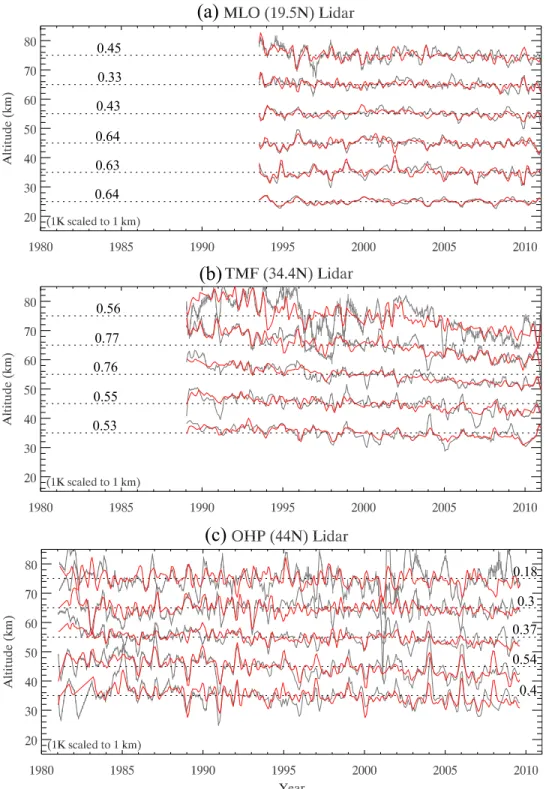
[9] Figures 2a, 2b, and 2c show the time series (plotted for

every other altitude) of the deseasonalized monthly mean temperature (black) for the three different lidar data sets at MLO, TMF, and OHP, respectively. The red superimposed curves are the corresponding reconstructed linear regression fits obtained by summing the trend, solar cycle, aerosol, ENSO, and QBO components, without the residuals. Also, the square of the correlation coefficient between the red and black curves is shown for each altitude and represents the fraction of the variance explained by the regression fit. The linear regression analysis generally captures the longer timescale variability with the best fitting for the MLO data set (>60% variance in the stratosphere and >30% in the mesosphere accounted for) but the worst fitting for OHP (40%–50% variances in the stratosphere while only 18% in the upper mesosphere accounted for), suggesting the increased intra‐annual and interannual variability at the higher latitude. A cooling trend is clear in the stratosphere and lower meso-sphere at both TMF and OHP and in the upper mesomeso-sphere at TMF. Lower signal‐to‐noise ratios in the mesosphere clearly result in higher statistical uncertainties, especially in the upper mesosphere, which cause more uncertainty in the regression fits in this region. In the mesosphere, the temper-ature tides become significant. However, the tidal effect was not large in the case of NDACC lidar data sets because even if the time of measurements changed from one day to another due to weather conditions, the starting measurement was always close to the beginning of the night, and integration of several hours smoothed out such effects [Keckhut et al., 1996; Leblanc et al., 1999].

3.

Temperature Trend

[10] Figures 3a, 3b, and 3c show the annual mean profiles

of the temperature trend derived from the lidar data sets at MLO, TMF, and OHP, respectively. For comparison, we also plotted the previously published annual trends near the lidar locations derived from the 1979–2005 SSU zonal mean data set by Randel et al. [2009], the 1991–2005 HALOE zonal mean data set by Remsberg [2009], and the 1969–1991 rocketsonde data sets by Keckhut et al. [1999]. A small cooling trend of ∼0.5 ± 0.5 K/decade was found between 30 and 60 km in the MLO lidar data set, in good agreement with the trends derived from SSU and HALOE at 20°N, and rocketsondes at Barking Sands (22°N) (except in the lower mesosphere, where rocketsondes had a large cooling trend). Note here that the rocketsonde time period has no overlap at all with the MLO lidar time period. At TMF, a cooling trend of∼2–4 K/decade, increasing with altitude up to 65 km, is consistent with the rocketsonde trend at Point Mugu (34°N) but almost twice the SSU and HALOE trends at 35°N. The stratospheric trend at OHP (−2 K/decade) is comparable

Table 1. Characteristics of the Three Rayleigh Lidar Data Sets

Data Sets Latitude, Longitude Duration

Regular Operating Hours per Night

Total Number of Nights

MLO 19.5°N, 55.6°W 1993.07–2010.12 2 2183

TMF 34.4°N, 117.7°W 1989.01–2010.12 2 2113 OHP 43.9°N, 5.7°E 1981.01–2009.08 4–10 3699

Figure 1. Histogram plot of the number of routine opera-tion nights in each month. The dotted line marks the mini-mum number of nights required for considering a valid monthly average from observations.

to the trend at TMF (−2 to −3 K/decade) and slightly larger than the SSU trend; but the mesospheric cooling trend at OHP is much smaller,∼2–3 times smaller than the HALOE trend, possibly because the data comes from different time periods: 1991–2005 for HALOE, 1982–2009 for OHP lidar. Figures 4a, 4b, and 4c show the seasonal variability of the temperature trend at MLO, TMF, and OHP, respectively. No

significant trend was found at MLO for any season. At TMF the temperature cooling trend was found to be significant at all altitudes with a maximum of∼3–4 K/decade in the upper stratosphere in spring and fall and∼4 K/decade in the winter mesosphere. Similarly, a summertime cooling trend with a maximum of ∼3 K/decade in the upper stratosphere was observed to be significant at OHP.

Figure 2. The selective time series of deseasonalized monthly mean temperature (black) shown at 10 km intervals and their corresponding linear regression fitting results (red) for three different lidar data sets at (a) MLO, (b) TMF, and (c) OHP. The temperature perturbation scale is 1 K km−1. The numbers above each dashed line denote the square of correlation coefficient between the red and black curves.

[11] The temperature cooling trends in the middle and

upper stratosphere observed by the Rayleigh lidars at TMF and OHP are generally larger than earlier satellite observa-tions [Remsberg, 2009; Randel et al., 2009]. This is not the case for the MLO lidar trend, which agrees very well with previous results. Using the historic rocketsonde data sets, both Dunkerton et al. [1998] and Keckhut et al. [1999] found a significant cooling trend of ∼1.7 K/decade in the stratosphere above 30 km when averaging multiple data sets from the tropics to the midlatitudes. Chemistry climate model (CCM) simulations of the stratospheric cooling trend with contributions from well‐mixed greenhouse gases and

ozone depletion are comparable to the early satellite and radiosonde results [Eyring et al., 2006; Austin et al., 2009]. Stratospheric water vapor, an important radiative consti-tuent, was previously observed to be increasing at a rate of 1–2% yr−1 _{in the upper stratosphere [Nedoluha et al.,}

1998]. This increase could also contribute significantly to the stratospheric cooling trend, as suggested by Rind and Lonergan [1995]. However, observations now suggest that water vapor did not continue to increase in the stratosphere [Solomon et al., 2010] and mesosphere [Nedoluha et al., 2003] during the last decade. The temperature trends revealed from long‐term data sets observed by ground‐based and

Figure 4. Seasonal variability of the temperature trend at (a) MLO, (b) TMF, and (c) OHP. The shaded regions in Figures 4a, 4b, and 4c indicate that the results are not significant at a 2s confidence level, while the dashed contour lines denote negative values and the solid lines denote positive values.

Figure 3. Annual mean profiles of the temperature trend at (a) MLO, (b) TMF, and (c) OHP, and com-parison with previous publications for the annual trend near lidar latitudes derived from SSU zonal mean (1979–2005), HALOE zonal mean (1991–2005), and rocketsonde (1969–1991) data sets. The dashed curves denote the lidar trend, and the horizontal bars indicate a 1s confidence level. The diamonds, stars, and plus signs denote SSU, HALOE, and rocketsonde trends, respectively.

spaceborne instruments at different locations typically show larger variability in the mesosphere than in the stratosphere [Keckhut et al., 1999; Beig et al., 2003]. Model simulations suggested a cooling trend of a few degrees per decade in the lower and middle mesosphere induced by doubled CO2

concentration and other major greenhouse gases [Beig et al., 2003; Schmidt et al., 2006].

[12] Using HALOE ozone 1991–2005 data sets,

Remsberg [2009] found that the ozone linear trend in the upper stratosphere and mesosphere was nearly zero. This was further confirmed in analyses of the long‐term NDACC lidar ozone data sets by Steinbrecht et al. [2009], who showed that the ozone density in the upper stratosphere started to increase only slightly after 1995. This change in the ozone trend could significantly affect the temperature trend in the middle atmosphere [Schwarzkopf and Ramaswamy, 2008; Laštovička, 2009]. Randel et al. [2009] also found relatively constant stratospheric temperature anomalies during 1995–2005 from their SSU data set. To explore the possible change in the temperature trend after 1995, in Figure 5 we plot the annual mean profiles of the temperature trend derived from the OHP data set during three different time periods (1981–2009, 1981–1994, and 1995–2009) (Figure 5a) and from three different lidar data sets during a single time period (1995–2009) (Figure 5b). The cooling trend below 60 km at OHP during 1995–2009 (≤0.8 K/decade) is much smaller than the trend at the same altitudes during 1981–1994 (∼2–3 K/decade), which is coincident with the stratospheric ozone trend change after 1995 and the slight decrease of water vapor over the past decade. Meanwhile the cooling trend during 1995–2009 at both MLO and OHP was much smaller than the trend at TMF. We have no further explanation for the large cooling trend found at TMF.

4.

Temperature Response to the 11 Year

Solar Cycle

[13] In addition to the temperature trend retrieved from

long‐term lidar data sets, we also extracted the temperature response to the 11 year solar cycle. Figures 6a, 6b, and 6c show the corresponding annual mean profiles of the solar cycle signals at MLO, TMF, and OHP, respectively, and how they compare with the previously published results for latitudes similar to the lidar locations obtained from the 1979–2005 SSU data set [Randel et al., 2009] and the 1991–2005 HALOE data set [Remsberg, 2009]. Note here that we converted the unit of K/sol max‐min given by both Randel et al. [2009] and Remsberg [2009] to K/100 F10.7. A positive correlation to the solar flux was observed at all altitudes over MLO with a maximum value of ∼1.0 ± 0.6 K/100 F10.7 near 35 and 55 km. At TMF a near‐zero response was found in the upper stratosphere, while a large response in the mesosphere increased linearly with altitude from ∼0.0 ± 0.7 K/100 F10.7 at 50 km to ∼3 ± 1.4 K/ 100 F10.7 at 75 km. At OHP the annual mean profile shows a small negative response of∼0.5 ± 0.8 K/100 F10.7 in the upper stratosphere and a positive response in the meso-sphere with a maximum value of ∼1.8 ± 0.7 K/100 F10.7 near 60 km. Comparisons of the lidar results with satel-lite results show very good agreement, except above 70 km at OHP.

[14] The rocketsonde data sets in the tropics and

sub-tropics revealed a positive temperature response to the solar cycle with a value of ∼1–2 K/100 F10.7 in the strato-sphere and∼2 K/125 F10.7 in the mesosphere [Dunkerton et al., 1998; Keckhut et al., 2005], slightly larger than the MLO lidar result (≤1 K/100 F10.7). The 11 year cycle of solar flux could primarily impact stratospheric ozone through photochemistry and thus affect stratospheric temperature [Ramaswamy et al., 2001]. The NCAR Whole Atmosphere Community Climate Model (WACCM) simulations also predicted a positive response of less than 1 K/125 F10.7 in the stratosphere [Marsh et al., 2007]. A recent review compared the updated results extracted from multiple data sets and found a positive response within a few K/125 F10.7 in the Northern Hemisphere subtropical and midlatitude mesosphere [Beig et al., 2008]. In general, quite good agreements were found for the middle atmosphere tem-perature response to solar cycle derived from various data sets.

[15] Figures 7a, 7b, and 7c show the seasonal variability of

the temperature response to the 11 year solar cycle at MLO, TMF, and OHP, respectively. A notable and significant fea-ture was found over OHP, exemplified by a negative response in the winter upper stratosphere (∼2.3 ± 0.9 K/100 F10.7 near 40 km) and a corresponding positive response in the middle mesosphere (∼3.2 ± 1.0 K/100 F10.7 near 60 km), which is generally consistent with the findings of Keckhut et al. [2005] based on the OHP lidar data set for 1979–2001. This winter response could be decadal variability, which is either truly due to the solar cycle or comes from something else and aliases in the solar cycle. In addition, a positive response of ∼2.5 ± 0.8 K/100 F10.7 in the summer mesosphere at OHP was also shown to be significant. In the Northern Hemi-sphere midlatitudes, the rocketsonde data sets showed a negative response to the 11 year solar cycle with an ampli-tude of∼2–3 K/125 F10.7 in the stratosphere [Keckhut et al., 2005], considerably stronger than the negative response with amplitude of∼0.5 K/125 F10.7 obtained from an early SSU satellite data set for 1979–1995 [Ramaswamy et al., 2001]. Using the ECMWF ER‐40 data set, Frame and Gray [2010] found a dominant positive response in the lower‐latitude stratosphere and a negative response in the higher‐latitude upper stratosphere in the Northern Hemisphere winter, con-sistent with lidar observations at OHP.

[16] The differences in temperature response to solar cycle

between the different data sets may have been due to their different time periods and geographical locations. To investigate this, we plotted the annual mean profiles of the temperature response to the 11 year solar cycle derived from the OHP data sets during three different periods (1981– 2009, 1981–1994, and 1995–2009) (Figure 8a) and at three different lidar locations during a single period (1995–2009) (Figure 8b) for comparison. In the upper stratosphere at OHP, the temperature response (∼2 K/100 F10.7) was neg-ative in 1981–1994 but positive in 1995–2009 and vice versa in the upper mesosphere. During the 1995–2009 period the temperature response in the stratosphere suggests a posi-tive correlation (1–2 K/100 F10.7) at all three locations, while in the upper mesosphere we found a positive response at TMF (2–4 K/100 F10.7) but a negative one at OHP (∼2 K/100 F10.7).

[17] To illustrate the opposite temperature response in the

upper stratosphere at OHP during the different solar cycles, Figure 9 shows the time series of stratospheric temperature anomalies (solid curve) at OHP averaged over 30–50 km, smoothed with a 3‐month window, and overlaid with the normalized F10.7 cm solar radio flux (dashed curve). It is clear that the temperatures were higher during the 1984– 1987 solar minimum than during the 1989–1992 solar maximum, especially in winter. In the following cycle, the temperatures were clearly lower during the solar minima in 1994–1997 and 2007–2009 than during the solar maximum in 2000–2002. The strong temperature peaks during the winters of 2003–2004 and 2005–2006 were likely related to

the strong sudden stratospheric warmings (SSWs) [Manney et al., 2008]. In addition, we note that a large temperature cooling trend (∼2 K/decade) during 1981–1994 but a near‐ zero trend during the 1995–2009 period were also found, coincident with the slight increase in upper stratospheric ozone density after 1995 observed by collocated ozone lidar [Steinbrecht et al., 2009].

[18] The opposite temperature response to the 11 year

solar cycle in the stratosphere and mesosphere found at OHP suggested that dynamical effects could play an important role in altering the sign of the response, as suggested by early modeling work [Balachandran and Rind, 1995]. It may also be related to planetary wave activity that could

Figure 6. As in Figure 3 but for the temperature response to the 11 year solar cycle.

Figure 5. Annual mean profiles of the temperature trend derived from the data sets (a) during three dif-ferent periods at OHP and (b) during 1995–2009 at three difdif-ferent lidar locations.

propagate upward into the upper stratosphere in the North-ern Hemisphere wintertime [Keckhut et al., 2005] and cause the significant SSW events in some winters [Gray et al., 2004; Hampson et al., 2005]. Using a mechanistic model, Hampson et al. [2005] found that the extratropical temperature response to the solar cycle is similar to that in the tropics if planetary wave (PW) forcing is either weak (which corresponded to no or weak SSW induced by PWs) or strong (which corresponded to SSW at both solar mini-mum and maximini-mum). However, if reasonable (intermediate) PW forcing is applied, the extratropical temperature solar signal in winter is fully reversed (negative response in the winter stratosphere). This is because the winter SSW induced by intermediate PW forcing occurs more frequently during solar minimum than during solar maximum. Winter SSW was usually accompanied by prior mesospheric cool-ing [Liu and Roble, 2002], which may have contributed to the observed opposite responses between the stratosphere and mesosphere.

[19] Further, the occurrence frequency of SSW is also

sensitive to both the solar condition (maximum or mini-mum) and the equatorial Quasi‐Biennial Oscillation (QBO) phase (westerly and easterly) [Labitzke, 1987]. The zonal mean zonal wind anomalies associated with both the QBO and the solar cycle are likely to play an important role in influencing the Northern Hemisphere (NH) winter strato-spheric polar vortex [Gray et al., 2004]. Holton and Tan [1980, 1982] found that the NH winter polar vortex is more disturbed by planetary waves during the QBO’s easterly phase than during its westerly phase. Using an idealized model ECMWF ERA‐40 data set, Gray et al. [2004] showed that during the solar minimum–QBO east-erly, the equatorial easterly zonal wind was reinforced, while it was weakened or canceled out during solar maxi-mum–QBO easterly and solar minimaxi-mum–QBO westerly. Camp and Tung [2007] found that the SSWs could occur during the QBO easterly phase at both solar maximum and minimum. The lowest occurrence frequency of SSWs was found during the QBO westerly phase and solar minimum

Figure 8. As in Figure 5 but for the 11 year solar cycle. Figure 7. As in Figure 4 but for the 11 year solar cycle.

condition. Therefore, the occurrence frequency of SSWs associated with the solar cycle and the QBO may influence the extratropical winter temperature response to the 11 year solar cycle. However, detailed studies of the occurrence frequency of SSWs under solar maximum and minimum conditions and during the QBO westerly‐easterly phases are complicated, and coordination with reanalysis data sets, satellite data sets, and model simulation is necessary to fully understand the mechanism.

[20] On the other hand, major volcanic eruptions, such as

El Chichón (April 1982) and Mount Pinatubo (June 1991), both happening near the solar maximum, directly induce significant transient warming events in the stratosphere [Ramaswamy et al., 2001; Randel et al., 2009] and indi-rectly affect the global temperature at the surface [Thompson et al., 2009], in the mesosphere [Keckhut et al., 1995], and even in the lower thermosphere [She et al., 1998]. This indirect effect on the temperature could persist much longer than expected. For example, the surface temperature cooling [Thompson et al., 2009] and mesopause temperature warm-ing [She et al., 1998] related to the Mount Pinatubo eruption may have lasted through 1998. The lidar temperature response to volcanic aerosol optical depth has similar results to that discussed in a previous paper [Keckhut et al., 1995]. Although we have included the time series of stratospheric aerosol optical depth in our regression fitting, thus repre-senting the major volcanic eruptions, the trend and solar cycle results may still be slightly disturbed by the indirect effect of major volcanic eruptions.

5.

Summary

[21] Using the long‐term temperature data sets obtained

with Rayleigh lidars at three different locations within the NDACC (MLO, Hawaii (19.5°N); TMF, California (34.4°N); OHP, France (43.9°N)), we studied the middle atmosphere temperature trend and temperature response to the 11 year solar cycle. The multiple linear regression analysis was used to extract the interannual signals from deseasonalized monthly mean temperature profiles. The cooling trend was found to be 2–3 K/decade in the middle and upper strato-sphere at both TMF and OHP, while ≤0.5 ± 0.5 K/decade

at MLO. Comparisons of these results with previously published trends derived from SSU and HALOE satellites and rocketsondes show generally good agreements, while a greater discrepancy between lidar and satellite cooling trends was found in the mesosphere at both TMF and OHP, with lidar trends twice as big at TMF (3–4 K/decade) but 2–3 times smaller at OHP (≤1 K/decade) than HALOE trends. The cooling trend in the upper stratosphere at OHP was much larger during the 1981–1994 period than during the 1995–2009 period, consistent with the slight increase of upper stratospheric ozone density after 1995 and the decrease of water vapor over the past decade.

[22] On the other hand, a significant temperature response

to the 11 year solar cycle was found in all three lidar data sets, with a positive response of≤1 K/100 F10.7 at MLO, linearly increasing positive response from near zero at 50 km to∼3.0 ± 1.4 K/100 F10.7 at 75 km at TMF, and a small negative response of ∼0.5 ± 0.8 K/100 F10.7 in the upper stratosphere at OHP coupled with a positive response of∼1.8 ± 0.7 K/100 F10.7 near 60 km. The lidar–solar cycle correlations agree well with satellite results. The winter negative response in the upper stratosphere at OHP corre-sponds with the winter positive response in the middle mesosphere, which is likely related to planetary wave activity and the occurrence frequency of SSWs influenced by the solar cycle and the QBO. Further, we found that the tem-perature response at OHP was negative in the upper strato-sphere during 1981–1994 while positive during 1995–2009, and vice versa in the upper mesosphere, possibly suggesting a different occurrence frequency of SSWs in winter during the different solar cycles. The apparent temperature response to the solar cycle observed with lidar may be not a direct solar cycle response at all but may instead come from the modulated random occurrence of SSWs, volcanoes, or some other decadal variability that aliases into the apparent solar cycle response.

[23] Acknowledgments. The research described in this paper was carried out at the University of Science and Technology of China, with support from the National Natural Science Foundation of China grants 40974084, 41074108, and 41025016, the specialized research fund for

Figure 9. Time series of the stratospheric temperature anomalies (solid curve) at OHP averaged over 30–50 km, smoothed with a 3 month window and overplotted with the normalized F10.7 cm solar radio flux (dashed curve). The reversed correlation during 1982–1992 is emphasized with the green solid curve.

State Key Laboratories, and the Chinese Academy of Sciences Hundred Talent program, and at the California Institute of Technology under an agreement with the National Aeronautics and Space Administration. The Rayleigh lidar long‐term operations are performed within the NDACC net-work, and the temperature data sets are available on the NDACC website: http://www.ndsc.ncep.noaa.gov/. Observatory of Haute Provence NDACC activities are supported by the Institute National des Sciences de l’Univers, the Centre National Études Spatiales, and the European Space Agency (ESA) through the Envisat Quality Assessment with Lidar ESA project (EQUAL), and long‐term investigations are funded by the European Integrated Project Geomon (contract FOP6‐2005‐Global‐4‐036677).

References

Austin, J., et al. (2009), Coupled chemistry climate model simulations of stratospheric temperatures and their trends for the recent past, Geophys. Res. Lett., 36, L13809, doi:10.1029/2009GL038462.

Balachandran, N. K., and D. Rind (1995), Modeling the effects of UV variability and the QBO on the troposphere–stratosphere system. Part I: The middle atmosphere, J. Clim., 8, 2058–2079, doi:10.1175/1520-0442(1995)008<2058:MTEOUV>2.0.CO;2.

Beig, G., et al. (2003), Review of mesospheric temperature trends, Rev. Geophys., 41(4), 1015, doi:10.1029/2002RG000121.

Beig, G., J. Scheer, M. G. Mlynczak, and P. Keckhut (2008), Overview of the temperature response in the mesosphere and lower thermosphere to solar activity, Rev. Geophys., 46, RG3002, doi:10.1029/2007RG000236. Brasseur, G. (1993), The response of the middle atmosphere to long‐term and short‐term solar variability: A two‐dimensional model, J. Geophys. Res., 98(D12), 23,079–23,090, doi:10.1029/93JD02406.

Camp, C. D., and K.‐K. Tung (2007), The influence of the solar cycle and QBO on the late‐winter stratospheric polar vortex, J. Atmos. Sci., 64, 1267–1283, doi:10.1175/JAS3883.1.

Dunkerton, T. J., D. P. Delisi, and M. P. Baldwin (1998), Middle atmo-sphere cooling trend in historical rocketsonde data, Geophys. Res. Lett., 25(17), 3371–3374, doi:10.1029/98GL02385.

Eyring, V., et al. (2006), Assessment of temperature, trace species, and ozone in chemistry‐climate model simulations of the recent past, J. Geophys. Res., 111, D22308, doi:10.1029/2006JD007327.

Frame, T. H. A., and L. J. Gray (2010), The 11‐yr solar cycle in ERA‐40 data: An update to 2008, J. Clim., 23, 2213–2222, doi:10.1175/ 2009JCLI3150.1.

Gray, L. J., S. Crooks, C. Pascoe, S. Sparrow, and M. Palmer (2004), Solar and QBO influences on the timing of stratospheric sudden warmings, J. Atmos. Sci., 61, 2777–2796, doi:10.1175/JAS-3297.1.

Gray, L. J., et al. (2010), Solar influences on climate, Rev. Geophys., 48, RG4001, doi:10.1029/2009RG000282.

Hampson, J., P. Keckhut, A. Hauchecorne, and M. L. Chanin (2005), The effect of the 11‐year solar cycle on the temperature in the upper strato-sphere and mesostrato-sphere: Part II. Numerical simulations and the role of planetary waves, J. Atmos. Sol. Terr. Phys., 67, 948–958, doi:10.1016/ j.jastp.2005.03.005.

Hauchecorne, A., and M. L. Chanin (1980), Density and temperature pro-files obtained by lidar between 35 and 70 km, Geophys. Res. Lett., 7(8), 565–568, doi:10.1029/GL007i008p00565.

Holton, J. R., and H.‐C. Tan (1980), The influence of the equatorial Quasi‐ Biennial Oscillation on the global circulation at 50 mb, J. Atmos. Sci., 37, 2200–2208, doi:10.1175/1520-0469(1980)037<2200:TIOTEQ>2.0. CO;2.

Holton, J. R., and H.‐C. Tan (1982), The Quasi‐Biennial Oscillation in the Northern Hemisphere lower stratosphere, J. Meteorol. Soc. Jpn., 60, 140–148.

Hood, L. (2004), Effects of solar UV variability on the stratosphere, in Solar Variability and Its Effect on the Earth’s Atmosphere and Climate System, Geophys. Monogr. Ser., vol. 14, edited by J. Pap et al., pp. 283–303, AGU, Washington, D. C.

Keckhut, P., A. Hauchecorne, and M. L. Chanin (1995), Midlatitude long‐ term variability of the middle atmosphere: Trends and cyclic and episodic changes, J. Geophys. Res., 100(D9), 18,887–18,897, doi:10.1029/ 95JD01387.

Keckhut, P., et al. (1996), Semidiurnal and diurnal temperature tides (30–55 km): Climatology and effect on UARS‐LIDAR data comparisons, J. Geophys. Res., 101(D6), 10,299–10,310, doi:10.1029/96JD00344. Keckhut, P., F. J. Schmidlin, A. Hauchecorne, and M. L. Chanin (1999),

Stratospheric and mesospheric cooling trend estimates from U.S. rocket-sondes at low latitude stations (8°S–34°N), taking into account instru-mental changes and natural variability, J. Atmos. Sol. Terr. Phys., 61, 447–459, doi:10.1016/S1364-6826(98)00139-4.

Keckhut, P., et al. (2004), Review of ozone and temperature lidar valida-tions performed within the framework of the Network for the Detection

of Stratospheric Change, J. Environ. Monit., 6, 721–733, doi:10.1039/ b404256e.

Keckhut, P., C. Cagnazzo, M.‐L. Chanin, C. Claud, and A. Hauchecorne (2005), The 11‐year solar‐cycle effects on the temperature in the upper stratosphere and mesosphere: Part I—Assessment of observations, J. Atmos. Sol. Terr. Phys., 67, 940–947, doi:10.1016/j.jastp.2005.01.008.

Labitzke, K. (1987), Sunspots, the QBO, and the stratospheric temperature in the north polar region, Geophys. Res. Lett., 14(5), 535–537, doi:10.1029/GL014i005p00535.

Laštovička, J. (2009), Global pattern of trends in the upper atmosphere and ionosphere: Recent progress, J. Atmos. Sol. Terr. Phys., 71, 1514–1528, doi:10.1016/j.jastp.2009.01.010.

Leblanc, T., I. S. McDermid, A. Hauchecorne, and P. Keckhut (1998), Evaluation of optimization of lidar temperature analysis algorithms using simulated data, J. Geophys. Res., 103(D6), 6177–6187, doi:10.1029/ 97JD03494.

Leblanc, T., I. S. McDermid, and D. A. Ortland (1999), Lidar observations of the middle atmospheric thermal tides and comparison with the High Resolution Doppler Imager and Global‐Scale Wave Model: 1. Methodol-ogy and winter observations at Table Mountain (34.4°N), J. Geophys. Res., 104(D10), 11,917–11,929, doi:10.1029/1999JD900007.

Li, T., T. Leblanc, and I. S. McDermid (2008), Interannual variations of middle atmospheric temperature as measured by the JPL lidar at Mauna Loa Observatory, Hawaii (19.5°N, 155.6°W), J. Geophys. Res., 113, D14109, doi:10.1029/2007JD009764.

Liu, H.‐L., and R. G. Roble (2002), A study of a self‐generated stratospheric sudden warming and its mesospheric–lower thermospheric impacts using the coupled TIME‐GCM/CCM3, J. Geophys. Res., 107(D23), 4695, doi:10.1029/2001JD001533.

Manney, G. L., et al. (2008), The evolution of the stratopause during the 2006 major warming: Satellite data and assimilated meteorological anal-yses, J. Geophys. Res., 113, D11115, doi:10.1029/2007JD009097. Marsh, D. R., R. R. Garcia, D. E. Kinnison, B. A. Boville, F. Sassi, S. C.

Solomon, and K. Matthes (2007), Modeling the whole atmosphere response to solar cycle changes in radiative and geomagnetic forcing, J. Geophys. Res., 112, D23306, doi:10.1029/2006JD008306.

Naujokat, B. (1986), An update of the observed Quasi‐Biennial Oscillation of the stratospheric winds over the tropics, J. Atmos. Sci., 43, 1873–1877, doi:10.1175/1520-0469(1986)043<1873:AUOTOQ>2.0.CO;2. Nedoluha, G. E., R. M. Bevilacqua, R. M. Gomez, D. E. Siskind, B. C.

Hicks, J. M. Russell III, and B. J. Connor (1998), Increases in middle atmospheric water vapor as observed by the Halogen Occultation Exper-iment and the ground‐based Water Vapor Millimeter‐wave Spectrometer from 1991 to 1997, J. Geophys. Res., 103(D3), 3531–3543, doi:10.1029/ 97JD03282.

Nedoluha, G. E., R. M. Bevilacqua, R. M. Gomez, B. C. Hicks, J. M. Russell III, and B. J. Connor (2003), An evaluation of trends in middle atmospheric water vapor as measured by HALOE, WVMS, and POAM, J. Geophys. Res., 108(D13), 4391, doi:10.1029/2002JD003332.

Ramaswamy, V., et al. (2001), Stratospheric temperature trends: Observa-tions and model simulaObserva-tions, Rev. Geophys., 39(1), 71–122, doi:10.1029/ 1999RG000065.

Randel, W. J., and F. Wu (1996), Isolation of the ozone QBO in SAGE II data by singular‐value decomposition, J. Atmos. Sci., 53, 2546–2559, doi:10.1175/1520-0469(1996)053<2546:IOTOQI>2.0.CO;2.

Randel, W. J., et al. (2009), An update of observed stratospheric tempera-ture trends, J. Geophys. Res., 114, D02107, doi:10.1029/2008JD010421. Remsberg, E. E. (2009), Trends and solar cycle effects in temperature ver-sus altitude from the Halogen Occultation Experiment for the mesosphere and upper stratosphere, J. Geophys. Res., 114, D12303, doi:10.1029/ 2009JD011897.

Rind, D., and P. Lonergan (1995), Modeled impacts of stratospheric ozone and water vapor perturbations with implications for high‐speed civil transport aircraft, J. Geophys. Res., 100(D4), 7381–7396, doi:10.1029/ 95JD00196.

Roble, R. G., and R. E. Dickinson (1989), How will changes in carbon dioxide and methane modify the mean structure of the mesosphere and thermosphere?, Geophys. Res. Lett., 16(12), 1441–1444, doi:10.1029/ GL016i012p01441.

Schmidt, H., G. P. Brasseur, M. Charron, E. Manzini, M. A. Giorgetta, T. Diehl, V. I. Fomichev, D. Kinnison, D. Marsh, and S. Walters (2006), The HAMMONIA chemistry climate model: Sensitivity of the mesopause region to the 11‐year solar cycle and CO2doubling, J. Clim.,

19, 3903–3931, doi:10.1175/JCLI3829.1.

Schwarzkopf, M. D., and V. Ramaswamy (2008), Evolution of strato-spheric temperature in the 20th century, Geophys. Res. Lett., 35, L03705, doi:10.1029/2007GL032489.

She, C. Y., S. W. Thiel, and D. A. Krueger (1998), Observed episodic warming at 86 and 100 km between 1990 and 1997: Effects of Mount

Pinatubo eruption, Geophys. Res. Lett., 25(4), 497–500, doi:10.1029/ 98GL00178.

Solomon, S., K. H. Rosenlof, R. W. Portmann, J. S. Daniel, S. M. Davis, T. J. Sanford, and G.‐K. Plattner (2010), Contributions of stratospheric water vapor to decadal changes in the rate of global warming, Science, 327(5970), 1219–1223, doi:10.1126/science.1182488.

Steinbrecht, W., et al. (2009), Ozone and temperature trends in the upper stratosphere at five stations of the Network for the Detection of Atmo-spheric Composition Change, Int. J. Remote Sens., 30, 3875–3886, doi:10.1080/01431160902821841.

Thompson, D. W. J., J. M. Wallace, P. D. Jones, and J. J. Kennedy (2009), Identifying signatures of natural climate variability in time series of global‐mean surface temperature: Methodology and insights, J. Clim., 22, 6120–6141, doi:10.1175/2009JCLI3089.1.

Wallace, J. M., R. L. Panetta, and J. Estberg (1993), Representation of the equatorial stratospheric Quasi‐Biennial Oscillation in EOF phase space, J. Atmos. Sci., 50, 1751–1762, doi:10.1175/1520-0469(1993) 050<1751:ROTESQ>2.0.CO;2.

X. Dou and T. Li, School of Earth and Space Sciences, University of Science and Technology of China, 96 Jinzhai Rd., Hefei, Anhui 230026, China. (litao@ustc.edu.cn)

A. Hauchecorne and P. Keckhut, Laboratoire Atmosphères, Milieux, Observations Spatiales, Institut Pierre‐Simon Laplace, Quartier des Garennes, 11 boulevard d’Alembert, F‐78280 Guyancourt, France.

T. Leblanc and I. S. McDermid, JPL Table Mountain Facility, California Institute of Technology, 24490 Table Mountain Rd., Wrightwood, CA 92397, USA.