Simultaneous observations of magnetopause flux transfer events and of their associated signatures at ionospheric altitudes

HAL Id: hal-00317452

https://hal.archives-ouvertes.fr/hal-00317452

Submitted on 14 Jun 2004

HAL is a multi-disciplinary open access

archive for the deposit and dissemination of

sci-entific research documents, whether they are

pub-lished or not. The documents may come from

teaching and research institutions in France or

abroad, or from public or private research centers.

L’archive ouverte pluridisciplinaire HAL, est

destinée au dépôt et à la diffusion de documents

scientifiques de niveau recherche, publiés ou non,

émanant des établissements d’enseignement et de

recherche français ou étrangers, des laboratoires

publics ou privés.

events and of their associated signatures at ionospheric

altitudes

K. A. Mcwilliams, G. J. Sofko, T. K. Yeoman, S. E. Milan, D. G. Sibeck, T.

Nagai, T. Mukai, I. J. Coleman, T. Hori, F. J. Rich

To cite this version:

K. A. Mcwilliams, G. J. Sofko, T. K. Yeoman, S. E. Milan, D. G. Sibeck, et al.. Simultaneous

observations of magnetopause flux transfer events and of their associated signatures at ionospheric

altitudes. Annales Geophysicae, European Geosciences Union, 2004, 22 (6), pp.2181-2199.

�hal-00317452�

Annales Geophysicae (2004) 22: 2181–2199 SRef-ID: 1432-0576/ag/2004-22-2181 © European Geosciences Union 2004

Annales

Geophysicae

Simultaneous observations of magnetopause flux transfer events and

of their associated signatures at ionospheric altitudes

K. A. McWilliams1, G. J. Sofko1, T. K. Yeoman2, S. E. Milan2, D. G. Sibeck3,7, T. Nagai4, T. Mukai5, I. J. Coleman6, T. Hori7, and F. J. Rich8

1_{Institute of Space and Atmospheric Studies, University of Saskatchewan, Saskatoon, Canada} 2_{Department of Physics and Astronomy, University of Leicester, Leicester, UK}

3_{NASA/GSFC, Greenbelt, Maryland, USA}

4_{Department of Earth and Planetary Sciences, Tokyo Institute of Technology, Tokyo, Japan} 5_{Institute of Space and Astronautical Science, Kanagawa, Japan}

6_{British Antarctic Survey, Cambridge, UK}

7_{Johns Hopkins University, Applied Physics Laboratory, Laurel, Maryland, USA} 8_{AFRL/VSBXP, Hanscom AFB, Massachusetts, USA}

Received: 4 March 2003 – Revised: 18 February 2004 – Accepted: 25 February 2004 – Published: 14 June 2004

Abstract. An extensive variety of instruments, including Geotail, DMSP F11, SuperDARN, and IMP-8, were mon-itoring the dayside magnetosphere and ionosphere between 14:00 and 18:00 UT on 18 January 1999. The location of the instruments provided an excellent opportunity to study in detail the direct coupling between the solar wind, the mag-netosphere, and the ionosphere. Flux transfer events were observed by Geotail near the magnetopause in the dawn side magnetosheath at about 4 magnetic local time during exclusively northward interplanetary magnetic field condi-tions. Excellent coverage of the entire dayside high-latitude ionosphere was achieved by the Northern Hemisphere Su-perDARN radars. On the large scale, temporally and spa-tially, the dayside magnetosphere convection remained di-rectly driven by the interplanetary magnetic field, despite the highly variable interplanetary magnetic field conditions, in-cluding long periods of northward field. The SuperDARN radars in the dawn sector also measured small-scale tempo-rally varying convection velocities, which are indicative of flux transfer event activity, in the vicinity of the magnetic footprint of Geotail. DMSP F11 in the Southern Hemisphere measured typical cusp precipitation simultaneously with and magnetically conjugate to a single flux transfer event signa-ture detected by Geotail. A study of the characteristics of the DMSP ion spectrogram revealed that the source plasma from the reconnection site originated downstream of the subsolar point. Detailed analyses of locally optimised coordinate sys-tems for individual flux transfer events at Geotail are con-sistent with a series of flux tubes protruding from the mag-netopause, and originating from a high-latitude reconnection site in the Southern Hemisphere. This high-latitude recon-nection site agrees with plasma injected away from the

sub-Correspondence to: K. A. McWilliams

(mcwilliams@dansas.usask.ca)

solar point. This is the first simultaneous and independent determination from ionospheric and space-based data of the location of magnetic reconnection.

Key words. Magnetospheric physics (energetic particles, precipitating; magnetosphere-ionosphere interactions) – Space plasma physics (magnetic reconnection)

1 Introduction

Magnetic reconnection is a fundamental process in the dy-namics of the magnetosphere, and the merging of the inter-planetary magnetic field (IMF) and the geomagnetic field on the dayside provides the primary mechanism for energy input into the magnetosphere from the solar wind. Understanding the nature of this reconnection process is a key to revealing the true nature of the interaction of the solar wind, the mag-netosphere, and the ionosphere. Several important questions that remain concern the nature of reconnection itself. Is re-connection a steady-state process? Is it episodic or bursty? Is it a combination of the two? If reconnection is transient in nature, then is it a large-scale phenomenon or is it small and patchy?

It is generally accepted that magnetic reconnection is the primary driver of magnetospheric and ionospheric convec-tion (Dungey, 1961). The Dungey picture is essentially a steady-state one, but the real interaction is time-dependent, most obviously because of the time-dependent nature of the external driver – the IMF – and possibly because of in-trinsic magnetopause instabilities. Haerendel et al. (1978) presented the first plasma and field observations from the frontside boundary layer, in the cusp region in particular, that were consistent with small-scale, transient reconnection at

the magnetopause. A bipolar variation of the magnetic field in the direction of the magnetopause normal has been inter-preted as due to a sharply kinked, newly-reconnected flux tube passing very near to the spacecraft (Russell and Elphic, 1978, 1979; Sonnerup, 1987; Farrugia et al., 1987).

In situ measurements of these reconnection bursts have been studied quite extensively (e.g. Haerendel et al., 1978; Russell and Elphic, 1978, 1979; Rijnbeek et al., 1984; Lock-wood and Wild, 1993; Kuo et al., 1995), and they have come to be known as flux transfer events (FTEs). Statistical stud-ies of FTEs from spacecraft data have revealed that they are common at all local times (Rijnbeek et al., 1984; Lockwood et al., 1995). FTEs occur predominantly during southward IMF conditions, but they can also occur when the IMF has a northward component (Kawano and Russell, 1997). North-ward events tend to occur when there is a dominant IMF By component (Kuo et al., 1995).

Because of the single-point nature of spacecraft measure-ments at the magnetopause, it is not possible to determine whether this spread over local times is due to many small bursts of reconnection scattered over the magnetopause or due to much larger FTEs covering large portions of the mag-netopause. One must also look to the ionosphere in the footprint of reconnection, where large-scale two-dimensional measurements of particles and fields are routinely made, to determine the nature of reconnection and the characteristic properties of FTEs. The early work of Elphic et al. (1990) demonstrated ionospheric flow bursts measured by EISCAT that followed FTEs observed by ISEE. The first magneti-cally conjugate measurements of an FTE by Equator-S and of ionospheric flow bursts by SuperDARN were presented by Neudegg et al. (1999), and the UV aurora measured by the VIS Earth camera in the vicinity of the reconnection footprint for this event was later discussed (Neudegg et al., 2001). More recently, Cluster observations have been com-bined with a variety of ground-based instruments (e.g. Wild et al., 2001; Lockwood et al., 2001a, 2001b). Statistically, the distribution of the repetition rates of pulsed ionospheric flows and poleward moving auroral forms is in agreement with the distribution of times between FTEs at the magne-topause (McWilliams et al., 2000).

The original prediction for the morphology of newly-reconnected field lines resulting from a flux transfer event was the flux rope model of Russell and Elphic (1978). In this scenario, a relatively short reconnection X-line forms a bulge in the magnetopause over which the magnetosheath and mag-netosphere fields are draped. The FTE flux tube itself was es-timated to have an area of about 10 RE(Russell and Elphic, 1979), but this was impossible to confirm due to the single-point nature of spacecraft measurements. This flux tube con-figuration would result in a dipolar variation of the compo-nent of the magnetic field normal to the magnetopause as the feature propagated past a spacecraft located near the bound-ary. A field-aligned current within the bulge would also give rise to a bipolar signature within the bulge. The ionospheric signature of such an FTE would be a patch of plasma moving with a velocity differing from that of the surrounding plasma

under the combined influence of the magnetic curvature and pressure gradient forces at the magnetopause (Goertz et al., 1985; Southwood, 1985, 1987).

An extension, quite literally, of the flux tube model is the two-dimensional reconnection pulse model in which the length of the reconnection line is not specified (Saunders, 1983; Southwood et al., 1988). The predicted ionospheric signature is conceptually similar to the flux tube model, but with the possibility of a feature with a much longer local time extent. This azimuthal extension of the reconnection region allows for the interpretation of large-scale ionospheric con-vection patterns in terms of FTEs (Cowley and Lockwood, 1992).

Recent multi-instrument studies of ionospheric signatures of FTEs demonstrated that transient magnetic reconnection can manifest itself as a global-scale peeling of magnetic flux tubes from the dayside magnetopause (Milan et al., 2000; McWilliams et al., 2001a; McWilliams et al., 2001b). Whilst the ionospheric data in these studies exhibited all the typical signatures of flux transfer events, which are often assumed to be associated with small-scale (of the order of a few thousand km at the magnetopause) reconnection bursts, the data were found to be the response to a locally transient phenomenon, both at the magnetopause and in the ionosphere, but each event developed in time to include the majority of the dayside ionosphere and magnetosphere.

In this study we will examine FTE signatures evident in a large number of data sets from a variety of instruments. Geotail provides evidence of FTEs at the magnetopause. We will examine localised boundary normal coordinates for each FTE, giving each FTE its own coordinate system. The orientation of these coordinate systems will be used to de-duce the location of the reconnection site and compare this with the predictions from the anti-parallel merging hypothe-sis (Crooker, 1979). The Geotail data will be compared with low-altitude reconnection signatures. SuperDARN was mon-itoring the large-scale response to IMF changes, as well as the localised transient features associated with the poleward convection following FTEs. DMSP measured the cusp parti-cle precipitation at the same time and magnetically conjugate to an FTE observed at Geotail. We will closely examine the energy-dispersed cusp ions, in particular the low-energy cut-off, from which we will reconstruct the field-aligned distri-bution of the plasma injected along the field line at the recon-nection site. The location of the reconrecon-nection site from the DMSP injected distribution will then be deduced and com-pared with the location determined from the Geotail analysis.

2 Instruments 2.1 Geotail

In this study Geotail magnetic field and plasma data from a dawn side magnetopause skimming orbit will be examined.

The magnetic field data presented in this study are from the magnetic field experiment (MGF) (Kokobun et al., 1994),

K. A. McWilliams et al.: Simultaneous FTEs and ionospheric signatures 2183 which includes dual tri-axial fluxgate magnetometers. The

fluxgate magnetometers have 7 ranges (from ±16 nT to ±65 536 nT), which are switched automatically. The samples are averaged to 16 vectors per second for the outboard sen-sor (mounted on a mast 7.15 m from the spacecraft spin axis) and to 4 samples per second for the inboard sensor (mounted on the same mast 5.12 m from the spin axis). In this study, 3-s averaged data were used.

Three-dimensional plasma velocities and moments are measured by the LEP-EA and LEP-SW sensor units of the low energy particle (LEP) experiment (Mukai et al., 1994) on Geotail. LEP-EA primarily measures hot magnetospheric electrons and positive ions in the energy ranges 8 eV to 38 keV for electrons and a few eV/Q to 43 keV/Q for ions. LEP-EA has a large geometrical factor, in order to measure tenuous magnetotail plasma. The fields of view of the elec-tron and ion analysers are 10◦×145◦, parallel to the satellite spin axis. Velocity measurements are calculated for every spacecraft spin (20 rpm), but due to telemetry constraints full three-dimensional velocity moments are only transmitted ev-ery fourth spin, with the count data being accumulated during the 4 spins.

Due to its large geometric factor LEP-EA is unable to mea-sure solar wind ions, particularly protons. LEP-SW is de-signed to measure solar wind ions in the energy range 0.1– 8 keV/Q. It has a 270◦spherical electrostatic analyser, whose field of view is 5◦×60◦. SW operates similarly to LEP-EA, but only the first of the velocity moments for each 4-spin data collection period are transmitted to the ground.

2.2 SuperDARN

The Super Dual Auroral Radar Network (SuperDARN) (Greenwald et al., 1995) is an international collaborative net-work of HF radars that monitors ionospheric plasma convec-tion over the majority of the northern and southern polar re-gions. Measurements from six of the Northern Hemisphere radars have been used in this study to produce global-scale ionospheric convection velocities in the dayside auroral zone and polar cap. The radars included in this study are listed in Table 1.

The SuperDARN radars use a multi-pulse transmission se-quence to sound 16 beams sequentially, forming a full scan that spans 52◦in azimuth. During the interval of interest on 18 January 1999, the radars are synchronised to perform a full 16-beam scan every two minutes. Measurements along each beam are taken in 75 range gates, which are 45 km in length, and the distance to the first gate is 180 km. The echoes from each range gate are processed through an au-tocorrelation function, from which one obtains the backscat-tered power, the mean Doppler velocity (an estimate of the ionospheric plasma drift velocity along the beam direction), and an estimate of the spectral width.

During the interval of interest the SuperDARN radars were monitoring the dayside auroral zone and polar cap. HF radars are particularly sensitive to plasma structures at the footprint of the magnetospheric reconnection region, where the soft

Table 1. The geographic locations and boresite headings clockwise

from geographic North of the SuperDARN radars used in this study.

Radar Code Latitude Longitude Heading

Saskatoon, Canada t 52.16◦N 106.53◦W 23.1◦ Kapuskasing, Canada k 49.39◦N 82.32◦W −12.0◦ Goose Bay, Canada g 53.32◦N 60.46◦W 5.0◦ Stokkseyri, Iceland w 63.86◦N 22.02◦W −59.0◦ þykkvibær, Iceland e 63.77◦N 20.54◦W 30.0◦ Hankasalmi, Finland f 62.32◦N 26.61◦E −12.0◦

particles precipitating along the magnetic field lines excite F-region irregularities, which act as a “hard target” in the dayside ionosphere (Milan et al., 1998).

2.3 DMSP

The DMSP F11 satellite, orbiting at 860 km altitude, has upward-looking charged particle flux and energy detectors amongst its complement of instruments. From the measured field-aligned plasma populations, the location and time vari-ation of high-latitude magnetospheric plasma regions can be inferred (e.g. Newell and Meng, 1992). In the present study, data from the Southern Hemisphere auroral zone measured by DMSP-F11 spacecraft will be examined. The spacecraft is three-axis stabilised with the particle detectors pointing to-wards the local zenith, directly away from the Earth. Elec-trostatic analysers measure electron and ion energies and fluxes from 32 eV to 30 keV in 20 logarithmically based steps (Hardy et al., 1985). The field of view of the particle spec-trometer is 2◦by 5◦for the 1–30 keV detector and 4◦by 5◦ for the 32–1000 eV detector. The ion driftmeter (Rich and Hairston, 1994) is part of a set of thermal plasma sensors on the DMSP, and it is capable of measuring the ion drifts in the horizontal and vertical planes perpendicular to the direction of travel.

3 Observations

3.1 Ionospheric convection responses to interplanetary magnetic field changes

The upstream IMF conditions are provided by IMP-8, which is located immediately upstream of the postnoon bow shock, as illustrated in Fig. 1. Upstream data from WIND was not available for this study, since WIND was located inside the magnetosphere. The GSM components of the IMF measured at IMP-8, presented in Fig. 2, were highly variable between 15:00 and 18:00 UT, but the changes in the components are due primarily to changes in the orientation of the IMF, rather than changes in the field strength. The plasma data (not shown) is steady throughout the interval, with the GSE x component of the solar wind velocity at about −350 km s−1 and the proton number density at about 10 cm−3.

Fig. 1. The trajectories of Geotail, WIND, and IMP-8 on 18

Jan-uary 1999 in GSE coordinates. IMP-8 was located immediately upstream of the bow shock, and Geotail was performing a mag-netopause skimming orbit of the dawn flank. A modelled magne-topause (Shue et al., 1997) and bow shock (Peredo et al., 1995), cal-culated for the plasma parameters listed in panel (a), are included for reference.

Estimates of the IMF delays from the IMP-8 spacecraft to the ionosphere were determined by analysis of the orienta-tion of the phase fronts that passed over the spacecraft using the method of Khan and Cowley (1999). The cross product of the IMF orientation (averaged over 10 min) before and af-ter the IMF discontinuity at 15:20 UT, for example, gives an estimate of the normal direction of the IMF phase front of

ˆ

n=[−0.737, −0.206, 0.644], referenced to GSE coordinates. The point at which the phase front intersects the subsolar axis is then calculated, and the propagation time from the sub-solar intersection point to the subsub-solar bow shock is deter-mined using the solar wind speed. The discontinuity is then propagated through the bow shock, and 2 min are added to account for the propagation of the signal through the mag-netosphere to the ionosphere (Khan and Cowley, 1999). At 15:20 UT the intersection of the phase front with the GSE ˆx

axis occurred at 4.7 RE. Because this is within the magne-tosphere, we must go back about 3 min to the time when the phase front passing through IMP-8 impinged upon the subso-lar bow shock. The transit time through the magnetosheath is estimated at approximately 11 min. Adding 2-min travel time to the ionosphere gives a total bow-shock-to-ionosphere delay of approximately 13 min, or 10 min from the measure-ment time at IMP-8 to the ionosphere response. Between 15:00 and 18:00 UT there were several changes in the phase front orientation, and each resulted in a delay from IMP-8 to the ionosphere in the range of 8–12 min, with the major-ity of the delays being 10 min. An estimate of the time delay of 10 min will be used to compare the ionospheric convection patterns measured in the ionosphere by SuperDARN with the IMF orientation at the IMP-8 spacecraft between 14:50 and 17:50 UT. Because the convection patterns are averages over 10 min, they should reflect changes in the IMF despite varia-tions in the estimated delay time of two minutes.

Excellent coverage of the dayside ionospheric convec-tion pattern was achieved by the Northern Hemisphere ar-ray of SuperDARN radars, and the dayside convection pat-tern is expected to respond directly to the changing orienta-tion of the IMF if the solar wind and the magnetosphere are coupled. Measurements from the six northern SuperDARN radars were used to create the convection maps. The Super-DARN convection velocity vectors in Fig. 3 were obtained by merging collocated measurements from the overlapping fields of view of the SuperDARN radars. The filled circles mark the centres of the areas encompassed by the overlap-ping radar beams and the lines denote the magnitude and di-rection of the merged convection velocities. In this case sev-eral radar scans were combined to produce convection pat-terns averaged over 10 min. These merge maps therefore re-veal the large-scale ionospheric response to the IMF changes, which occur on a scale of tens of minutes. The most imme-diate response in the ionosphere to the IMF orientation dur-ing reconnection is expected in the equatorward portion of the merged convection velocities. The IMF orientation for each merge map in Fig. 3 is marked by the dashed lines in Fig. 2, with the labels corresponding to the merge panel la-bels in Fig. 3. A quiet-time (Kp=0) auroral oval (Feldstein and Starkov, 1967) is plotted on each merge panel for refer-ence.

The IMF has a small northward component (+2 nT), a nearly zero Bx component, and a strong By component (+7 nT) until 15:20 UT. An example of the ionospheric con-vection pattern corresponding to this IMF orientation mea-sured between 14:50 and 15:00 UT (Fig. 3a) exhibits primar-ily azimuthal flow in the dawnward direction, as expected for strongly positive Byconditions.

At 15:20 UT the IMF becomes weakly southward (Bz∼−2 nT), and the By component remains dominantly positive (+6 nT). The corresponding ionospheric convection pattern measured between 15:30 and 15:40 UT responds to the southward turning, with poleward convection in Fig. 3b. There is still a component of dawnward flow, in response to the persistent positive Bycomponent.

K. A. McWilliams et al.: Simultaneous FTEs and ionospheric signatures 2185

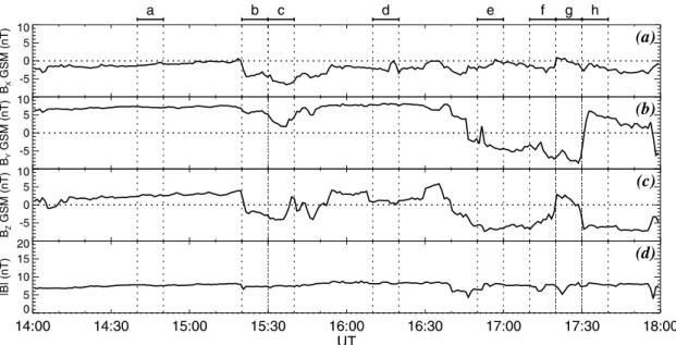
Fig. 2. (a) Bx, (b) By, (c) Bzmagnetic field components in GSM coordinates, and (d) the magnetic field strength from the IMP-8 spacecraft.

(a) 1450-1500 y z 12 18 (b) 1530-1540 z _y 18 (c) 1540-1550 y z 18 (d) 1620-1630 y z 80o 80o 70o 70o 18 1000 m/s (e) 1700-1710 1000 m/s 1000 m/s 1000 m/s 1000 m/s y z 12 06 (f) 1720-1730 z _y 06 (g) 1730-1740 y z 06 (h) 1740-1750 y z 80o 80o 70o 70o 06

Fig. 3. Two-dimensional convection velocities during selected intervals of interest. Dashed concentric circles represent contours of magnetic

latitude, and the straight dashed lines represent hours of magnetic local time, with 12 MLT at the top of the plots. The merged vectors were obtained by reconstructing a horizontal ionospheric convection velocity from two overlapping line of sight velocity components measured by two SuperDARN radars. The line of sight data were averaged over 10 min. The corresponding averaged IMF orientation in the Byand BzGSM plane is plotted in the upper right-hand corner of each panel, and each corresponding 10-min interval is marked at the top of Fig. 2, with the labels corresponding to the panel labels in this figure.

Fig. 4. The BzGSM component of the magnetic field measured at (a) Geotail (black line) and (b) IMP-8. The IMP-8 data has also

been plotted in red in panel (a), magnified by a factor of three and subjected to three time delays of 20 min, 15 min and 6 min, as indi-cated at the top of the figure.

At 15:30 UT the IMF By component becomes much weaker (+2 nT), while the Bzcomponent remained strongly southward (−4 nT). The poleward convection velocities are faster in the corresponding convection pattern (15:40– 15:50 UT; Fig. 3c). There is evidence of the dayside por-tion of the convecpor-tion reversal boundary in the dawn sector, typical of the southward IMF twin-cell convection pattern.

The IMF conditions between 16:10 and 16:20 UT are nearly identical to the initial configuration: weakly positive Bz (+1 nT), strongly positive By (+8 nT), and weakly neg-ative Bx (−2 nT). The corresponding convection pattern in Fig. 3d is very similar to the initial convection pattern in Fig. 3a. At approximately 80◦ magnetic latitude there is a strong dawnward flow with very little poleward convec-tion. Above 80◦there remain, however, vestiges of the strong poleward flow that echo those during the prior IMF orienta-tion.

Between 16:50 and 17:00 UT the IMF Bx component re-mains nearly zero, while the By component becomes nega-tive (−3 nT), and the Bzcomponent is southward with an av-erage value of about −3 nT. In the 17:00–17:10 UT panel of Fig. 3e, the low latitude flows into the polar cap in the corre-sponding ionospheric convection data in Fig. 3e are strongly duskward, and there are vestiges of dawnward flow at high latitudes. There is evidence of the dayside portions of the convection reversals of the simple twin cell vortical flow pat-terns.

During the 17:10–17:20 UT interval, the IMF By com-ponent had become more strongly negative (−6 nT), which was of similar magnitude to that of the Bz component. The associated convection pattern in the equatorward portion of the throat (Fig. 3f; 17:20–17:30 UT) continues to have a duskward component during this interval, while the

convec-tion further into the polar cap is less extensive than the pre-vious panel and is primarily poleward.

At 17:20 UT, the IMF Bz component sharply changed from negative (∼−5 nT) to weakly positive (+2 nT), last-ing until 17:30 UT, and the strongly negative Bycomponent (∼−7 nT) dominates during this interval. The corresponding ionospheric convection velocities in Fig. 3g exhibit nearly totally azimuthal duskward flow below 80◦ and very little backscatter further poleward. The prenoon convection rever-sal boundary is observed to cross local noon into the post-noon sector by about 2 h of local time.

The sudden positive turning of the IMF By component from −8 nT to +6 nT at 17:30 UT excites the convection pattern measured in Fig. 3h, in which the equatorward convection velocities have rotated from nearly azimuthally duskward to poleward and dawnward. The IMF Bz compo-nent was strongly negative at −6 nT. The prenoon convec-tion reversal boundary is no longer evident between 12 and 14 magnetic local time (MLT).

3.2 Geotail magnetopause encounters

The trajectory of the Geotail spacecraft from the dawnside magnetosphere into the magnetosheath at about 04:00 MLT (about 15 Earth radii downstream of the Earth) resulted in a prolonged series of magnetopause crossings of the dawn-side magnetopause. The GSM ˆz component of the mag-netic field measured by Geotail during its final magneto-sphere encounters is the black line in Fig. 4a. To elucidate comparison between the IMF and the magnetosheath field, which is expected to be compressed, the measured IMF data in panel (b) has been multiplied by a factor of three and has been subjected to three different delays (a 20-min de-lay until 15:02 UT, a 15-min dede-lay from 15:02 to 16:50 UT, and a 6-min delay after 16:50 UT). The scaled and delayed IMF data is the red line in panel (a). Prior to 14:54 UT, the z component of the Geotail magnetic field data oscil-lated rapidly between relatively steady northward orienta-tions (Bz∼12 nT), corresponding to the magnetosphere (e.g. 13:45 to 14:15 UT), and more variable intervals in the mag-netosheath, corresponding to the lagged IMP-8 observations (e.g. 14:10 to 14:30 UT). The presence of both field signa-tures are consistent with rapid boundary fluctuations over the spacecraft, and the plasma moment data during this interval (not shown) are consistent with the spacecraft passing rapidly in and out of the magnetosphere. At 14:54 UT the Geotail spacecraft passed out of the magnetosphere and remained, for the most part, in the magnetosheath.

A more detailed view of the field and plasma data mea-sured immediately following the last magnetopause crossing is presented in Fig. 5. The top three panels are the magnetic field components at Geotail; they have been converted into the traditional boundary normal coordinates obtained by a minimum variance analysis (Sonnerup and Scheible, 1998) on the 14:50–17:00 UT data as a whole. In this LMN co-ordinate system (Russell and Elphic, 1978), the direction of minimum magnetic field variance is defined as the boundary

K. A. McWilliams et al.: Simultaneous FTEs and ionospheric signatures 2187

Fig. 5. (a) B_l, (b) Bm, (c) Bnboundary normal (Russell and Elphic, 1978) magnetic field components, and (d) the magnetic field strength from Geotail. The boundary normal unit vector relative to GSM is [−0.277, 0.927, 0.253]. (e)–(g) The plasma velocity in the ˆx, ˆy, and ˆz GSM directions, respectively, (h) the plasma concentration, and (i) the ion temperature from the LEP-SW instrument on Geotail.

normal direction ˆn, the ˆmdirection is set orthogonal to ˆn with no component in the GSM ˆz direction, and the ˆl direc-tion completes the right-handed set. Roughly speaking, the

ˆ

mdirection points westward and the ˆl direction northward. Panel (d) is the magnetic field strength measured at Geotail. The bottom three panels of Fig. 5 are the GSE ˆx component of the plasma velocity, the plasma number density, and the ion temperature, respectively. The plasma data during this interval was measured by the LEP-SW instrument on Geo-tail, which may be less reliable in the magnetosheath, as well as when it is in the solar wind during highly disturbed con-ditions. However, the data can still be used qualitatively as verification of processes responsible for the measured mag-netic field signatures.

In Fig. 5c nine instances of a bipolar variation of Bn are evident, and these are marked by the vertical dashed lines. These boundary normal signatures were measured at the same time as transient increases in the magnetic field

strength (panel d), increases in the tailward speed of the plasma (panel e), decreases in the plasma number density (panel f), and increases in the plasma temperature (panel g). These signatures imply that the spacecraft was in the mag-netosheath, and flux tubes containing a mixture of magne-tosheath and magnetospheric plasma periodically convected past the spacecraft. It is important to note that the same boundary normal transformation was used for the extended interval of more than two hours of data presented in Fig. 5. The LMN boundary normal vectors in GSM coordinates are: ˆl=[0.07, −0.24, 0.97], ˆm=[−0.96, −0.29, 0.00], and

ˆ

n=[0.28, -0.93, -0.25]. Local boundary coordinates vary with time, depending on the shape of the magnetopause. Whilst the data presented in Fig. 5 are extremely useful in de-termining where the most obvious FTE features occur in the data, for our purposes it is essential to examine the localised boundary normal coordinates for several specific intervals in much greater detail, and this will be discussed in Sect. 4.2.

Fig. 6. The field components and strength for the FTE signature centred on 15:18 UT in (a) GSM coordinates, (b) boundary normal LMN

coordinates, and (c) local boundary normal IJK coordinates (solid line) and minimum variance coordinates (dashed line) (Sonnerup and Scheible, 1998).

4 Discussion

4.1 Upstream IMF and ionospheric convection

In Sect. 3.1 it was demonstrated that the dayside ionospheric convection pattern was responding directly to the orientation of the IMF. While the appropriate IMF delay changes by a minute or two due to slightly varying solar wind speed, changing orientations of phase fronts, and motion of the spacecraft, the correspondence between the IMF orientation and the direction of ionospheric convection on a time resolu-tion of 10 min in the dayside auroral zone and polar cap is as expected (e.g. Weimer, 1995; Ruohoniemi and Greenwald, 1996). When there was a southward IMF Bz component, there was poleward flow in the noon sector, tilted according to the orientation of the IMF Bycomponent. When the IMF Bz component was positive the By component became the dominant factor in determining the direction of flow in the throat of the convection pattern, with largely azimuthal flows developing.

According to the anti-parallel merging hypothesis (Crooker, 1979), magnetic reconnection under southward IMF conditions occurs on the closed field lines equatorward of the magnetic cusps. Magnetic reconnection under north-ward IMF conditions is expected to occur on the open field lines of the mantle, effectively stirring the open field lines in the polar cap and forming a so-called lobe convection cell in the polar cap. For northward IMF conditions no flux transfer from closed dayside field lines to open polar cap/mantle field lines is expected. For both positive and negative Bz the addition of a By component will shift the reconnection site in local time and latitude, and the addition of a strong enough Bycan create two reconnection sites at high latitudes away from the local noon. When Bzis weakly negative and

By is strong, the flows into the polar cap will have a large azimuthal component. The azimuthal flows in the dayside portion of a lobe cell (due to reconnection at high-latitudes on open field lines) can appear very similar to the azimuthal flows expected during high-latitude reconnection on closed field lines, expected when By is strong and Bz is weakly negative. More information is required about the location of the open-closed field line boundary and the particles that precipitate from the reconnection region in order to distinguish between reconnection on open or closed field lines at high latitudes. For the case presented here, we will attempt to resolve the uncertainty about the location of reconnection by comparing the ionospheric convection measurements with Geotail observations of FTEs and with DMSP F11 observations of ions precipitating along these newly-reconnected field lines.

Whilst the overall convection near the cusp responds as predicted on a time scale of tens of minutes in the present study, the particulars of the reconnection process and the cor-responding flow response remain at smaller temporal scales. This gives the opportunity for a more detailed analysis of Geotail magnetopause data, as well as DMSP particle data in the vicinity of the cusp footprint. Such an analysis should provide insight into the possible variations of the reconnec-tion process itself in the context of driven ionospheric con-vection flows from individual SuperDARN radars. The direct response to the IMF throughout the entire interval presented here with a consistent time delay implies direct coupling of the IMF and the solar wind. From the convection pattern alone, it is very difficult to determine if the reconnection is occurring on closed or open field lines at the magnetopause, but the convection patterns are vital to placing other mea-surements of reconnection in context.

K. A. McWilliams et al.: Simultaneous FTEs and ionospheric signatures 2189 4.2 Geotail FTEs in detail

The IMF delays to the ionosphere are relatively well-defined, due to the close proximity of IMP-8 to the Earth, but time delays to the Geotail spacecraft, which is located deep within the magnetosheath near the dawn-side magnetopause at about 4 MLT, are much more variable. In order to match up the large-scale magnetic field features in Fig. 4, it was necessary to impose 3 different IMF delays. When Geotail is largely within the magnetosphere (prior to 14:54 UT) a delay of 20 min is required, which is not unreasonable, consider-ing the 8-min propagation estimated to the subsolar point. After this time, Geotail is in the magnetosheath and mea-sures a field very similar to the IMF, but compressed, match-ing well the IMF field component multiplied by a factor of three. The IMF delay after Geotail’s final exit of the magne-tosphere at 14:54 UT is 15 min, and after 16:50 UT the delay is reduced to 6 min. This is not unexpected, as it has long been known that in general, the plasma flow in the tosheath increases with increasing distance from the magne-topause (e.g. Spreiter and Stahara, 1980). Changes in the ori-entation of the IMF will also produce different delays. Prior to 16:50 UT the orientation of the IMF in the ecliptic plane measured at IMP-8 was Bx negative and By positive. After 16:50 UT the IMF becomes largely azimuthal with Bxnear zero and By largely negative. The magnetic field that was detected at IMP-8 after 16:50 UT would have been further downstream in the dawn sector than the field measured prior to 16:50 UT, and therefore a shorter transit time to the space-craft after 16:50 UT is expected.

4.2.1 Local boundary normal coordinates

Following its exit from the magnetosphere at 14:54 UT, Geo-tail measured a series of signatures typical of FTEs passing near the spacecraft – bipolar field variations in the bound-ary normal direction, transient increases in the field strength, the antisunward velocity and the ion temperature, as well as transient decreases in plasma number density. These data suggest that a sequence of newly-reconnected flux tubes, on which there existed a mixture of magnetosheath and mag-netospheric plasma, passed by Geotail, which is situated in the downstream dawnside magnetosheath. As mentioned in Sect. 3.2, the boundary normal direction, used to calculate the LMN magnetic field components in Fig. 5, was an esti-mate over about two hours, but particular attention must be paid to each individual FTE, in order to accurately determine the boundary normal coordinates for each FTE traversal.

Localised boundary normal coordinates are less restrictive than the traditional LMN coordinates, in which ˆmmust have no component in the GSM ˆz direction. To facilitate the in-terpretation of the magnetic field variations for the FTEs, it is very useful to try to decouple the field components, start-ing from the minimum variance determination of the LMN boundary normal coordinates. The coordinate system is ro-tated until each orthogonal component contains a feature which is comprehensible in terms of FTE-type activity at the

magnetopause. An example of an easily decoupled event was centred on 15:18 UT and lasted for approximately two min-utes (see Fig. 5). There was a bipolar variation measured in the Bn component (in the LMN coordinate system), which is evident in Fig. 5, but the bipolar feature is also apparent in the other components of the magnetic field. By rotating the coordinate system, it is possible to confine the bipolar signature to a single component.

For each FTE signature the LMN boundary normal co-ordinate system was re-calculated for a much smaller time interval. From the GSM magnetic field data for the 15:18 UT event (Fig. 6a), the LMN coordinates were cal-culated based on the data between 15:16 and 15:20 UT. Geo-tail remained primarily in the magnetosheath, only skirt-ing the structures that caused the FTE signatures, and the minimum variance technique (Sonnerup and Scheible, 1998) picked out approximately the magnetosheath field direction as the minimum variance direction. For the 15:18 UT event, a rotation of 90◦about the minimum vari-ance ˆm direction yields the familiar bipolar signature in the ˆn direction, while retaining the restriction that ˆm has no component in the ˆz GSM direction. The boundary normal LMN coordinate system for the 15:18 UT event is defined with the unit vectors ˆl=[−0.65, −0.05, 0.76],

ˆ

m=[0.07, −0.997, 0.00], ˆn=[0.76,0.06,0.65], and the LMN magnetic field components are presented in Fig. 6b.

From this point, the coordinate system was rotated to de-couple the magnetic field signatures of the FTE. In local boundary coordinates, the restriction that the z component of ˆmbe zero no longer applies. The LMN coordinate sys-tem was rotated −170.5◦ _{about ˆmto minimise B}

m outside the FTE signature. Then the coordinate system was rotated by 169◦_{about the new ˆl to maximise the bipolar variation} in the new “Bn”. A rotation of 2◦about the resulting ˆnaxis minimises “Bm” outside the bipolar field variation.

These coordinate transforms define the new local bound-ary normal coordinates, and we call these new coordinates ˆi,

ˆ

j, and ˆk to distinguish them from the conventional LMN co-ordinates. The magnetic field data in IJK coordinates for the 15:18 UT event is presented in Fig. 6c. The localised IJK co-ordinates, referenced to the GSM coco-ordinates, are shown in Fig. 7, and the unit vectors are as follows: ˆi=[0.73,0.25,0.63],

ˆ

j=[0.10, −0.96, 0.27], ˆk=[0.67, −0.14, −0.73]. The decou-pled field components in this system are such that Biis nearly constant, Bj has a step function-like increase over the event, and the Bkvariation is bipolar. The IJK coordinate system is similar to that derived from the minimum variance technique (Sonnerup and Scheible, 1998), the field components from which are plotted as the dashed lines in Fig. 6c. The mini-mum variance technique does not, however, completely de-couple the field components; for example, the step-function behaviour of Bj is still evident, but the field outside the step function does not tend to zero.

In the IJK coordinate system ˆi is approximately in the di-rection of the magnetosheath field, and ˆj is approximately normal to the magnetopause. Perhaps surprisingly, the direc-tion of the bipolar field oscilladirec-tion, ˆk, is not normal to the

Fig. 7. The localised boundary normal unit vectors for the 15:18 UT

FTE relative to the GSM coordinate system were ˆi=[0.73, 0.25, 0.63], ˆj=[0.10, −0.96, 0.27], ˆk=[0.67, −0.14, −0.73].

Fig. 8. An artistic rendering of a possible flux tube geometry that

would excite localised boundary normal field variations like those measured at 15:18 UT and presented in Fig. 6. Panel (a) portrays the event in a plane perpendicular to the magnetopause and panel (b) portrays the event in the plane of the magnetopause.

magnetopause, but rather it lies in the plane of the magne-topause. Nevertheless, as illustrated in Fig. 8, this would be expected for a flux tube protruding from the magnetopause, an FTE of the type originally illustrated by Russell and El-phic (1978).

Figure 8a is a view from above (+ˆz GSM) of the magne-tosheath adjacent to the dawn magnetopause as a flux tube passes the spacecraft in the direction of the magnetosheath flow. As the flux tube passes the spacecraft, the magnetome-ters will measure a step-like deflection in the ˆj direction, but the ˆi component is expected to remain relatively steady if it is aligned along the direction of the magnetosheath field. When looking at the magnetopause along the direction of the protruding flux tube, as illustrated in Fig. 8b, the flux tube passes below the spacecraft, and Geotail would detect a con-stant Bi, a step-function change in Bj, and a bipolar variation in Bk. The field compression over the event, the deflection of the field in a direction perpendicular to the flux tube, and the bipolar draping over the flux tube are consistent with previ-ous studies of FTEs (Sonnerup, 1987; Farrugia et al., 1987). The FTE signature passed the spacecraft in about 2 minutes, and the speed within the features was roughly 350 km/s ac-cording to LEP-SW, giving an approximate extent of 6–7 RE. This simple model can be applied to several of the FTEs, but those closest to the magnetopause and furthest into the magnetosheath are much more difficult to deconvolve. An example of a slightly more complicated case is centred on 15:06 UT (not shown). By applying the same localised co-ordinate transformation as that determined for the 15:18 UT event, one finds that there is still a constant Bi component, but in this case there is evidence of two consecutive bipolar oscillations, and the Bj component shows evidence of two consecutive step-like increases. It appears in this case that a pair of adjacent reconnected flux tubes passed near Geo-tail. In all cases, the plasma speed inside the FTE features was nearly 20% higher, from about 275 km/s to 325 km/s, and was of similar magnitude to that described for the event at 15:18 UT. In this series of FTEs, while some cases are more complicated, they generally satisfy the simple flux tube model.

The draping of the magnetosheath field, as determined from the localised boundary normal coordinates, has impli-cations for the location of the reconnection site. Under pos-itive ByIMF conditions, the antiparallel merging hypothesis (Crooker, 1979) predicts reconnection at high latitudes in the northern postnoon sector and in the southern prenoon sector. 4.2.2 Implications for the location of the reconnection site Figure 9 presents a comparison of solar wind, magnetopause, and ionospheric measurements taken between 14:00 and 18:00 UT on 18 January 1999, during the interval of FTEs. Panels (a) and (b) are the ˆy and ˆz GSM components of the IMF measured at IMP-8, respectively. The IMP-8 data has been plotted with a 10-min offset, which was found to be appropriate in Sect. 3.1 for delays to the ionosphere.

Panel (c) is the nonlocal boundary normal component of the magnetic field at Geotail (Bn), which is reproduced from Fig. 5, and the FTEs are marked with the verti-cal dashed lines. Ionospheric convection velocities mea-sured by the SuperDARN radars at Kapuskasing and Saska-toon are presented in panels (d) and (e), respectively. The

K. A. McWilliams et al.: Simultaneous FTEs and ionospheric signatures 2191

Fig. 9. Comparison of (a) and (b) the upstream IMF, (c) Geotail FTEs, and ionospheric convection velocities observed by (d) beam 9 at

range 49 of the Kapuskasing and by (e) beam 10 at range 55 of the Saskatoon SuperDARN radars. The magnetic footprint of the Geotail spacecraft is located in the Saskatoon-Kapuskasing field of view in the prenoon sector.

Saskatoon-Kapuskasing radar pair was located in the dawn sector between 6 and 12 MLT and the magnetic footprint of the Geotail spacecraft, calculated using the T96 magnetic field model (Tsyganenko and Stern, 1996), was located in the field of view of the two radars.

Throughout the interval (14:00–18:00 UT) the Kapuskas-ing radar, which was directed primarily antisunward, mea-sured a series of poleward moving regions of backscatter with velocities away from the radar, indicated by the arrows. These transient features were consistent across several adja-cent radar beams, including beam 7. The velocities measured along Kapuskasing beam 7 are colour coded such that nega-tive velocities (red-yellow) are flows away from the radar and positive (blue-green) towards. The location of Kapuskasing beam 7 is the blue beam in Fig. 3.

Similar poleward moving features were seen early on by STARE in 1978, and they were found to be closely

associ-ated with field-aligned plasma beams at the magnetopause measured by GEOS 2 (Sofko et al., 1979; Sofko et al., 1985), and since then these poleward moving radar auroral forms (PMRAFs) have been shown to be typical of the iono-spheric response to FTEs (e.g. Pinnock et al., 1995; Provan et al., 1998; McWilliams et al., 2000). The PMRAFs in the present study also have high backscattered power and high spectral widths (not shown), which are indicative of recon-nected field lines (Davies et al., 2002; McWilliams et al., 2001a). As the radar fields-of-view rotate towards magnetic local noon, the increased ionisation in the F-region results in more radar echoes. However, it is important to note that, even with changing backscatter conditions, PMRAFs are ob-served throughout the interval, regardless of the orientation of the IMF.

The easternmost beams of the Saskatoon radar were di-rected primarily azimuthally towards noon from the dawn

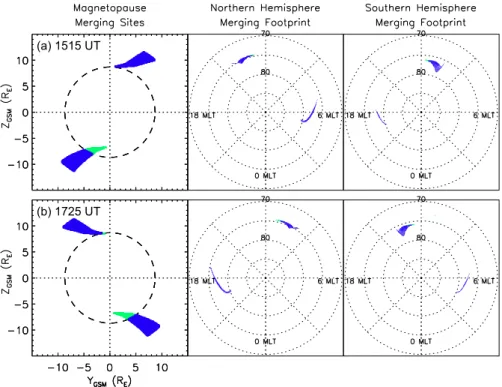
Fig. 10. The y-z GSM projection of the antiparallel merging regions on a modelled magnetopause, according to the method of Coleman et al.

(2001) for (a) 15:15 UT and (b) 17:25 UT. The dashed circle denotes the boundary between sub-Alfvénic and super-Alfvénic flow regions. The merging footprint plots illustrate where the antiparallel merging sites map down to the northern and southern ionospheres, as a function of magnetic latitude and local time.

sector during this interval. The Saskatoon radar was there-fore sensitive to azimuthal flows in the vicinity of the foot-print of reconnection and did not measure the PMRAFs, but periodic velocity fluctuations with a repetition rate of the or-der of several minutes are still evident in the data. Line-of-sight velocity data from beam 10, range 55 of the Saskatoon radar are presented in panel (e), and the location of this range cell is drawn in red in Fig. 3. The time scale of the velocity fluctuations is similar to the time between FTEs measured at Geotail and the time between PMRAFs measured by the Ka-puskasing radar. The slower variations of the order of tens of minutes are direct responses to changes in the IMF. When the IMF Bycomponent was strongly positive, the Saskatoon line-of-sight velocities were positive (towards the radar), or equivalently dawnward for this range gate. When the IMF Bycomponent was negative, the flows were directed towards local noon (away from the radar), as expected. This direct response to the IMF was discussed in terms of the merged convection velocities in Fig. 3. Both the line of sight data in Fig. 9 and the merged data in Fig. 3 are strongly suggestive of direct coupling of the IMF and the magnetospheric field via FTEs.

The Geotail FTEs and SuperDARN PMRAFs do not ex-hibit a one-to-one correspondence, but this is not unexpected, due to the highly localised nature of the Geotail data and the extensive SuperDARN coverage, which maps out to vast re-gions of the magnetosphere. An interesting study would be a detailed analysis of in situ measurements of FTEs

occur-ring under a variety of IMF conditions and the evolution of their footprints in the ionosphere viewed by pairs of overlap-ping SuperDARN radars. This type of study is beyond the scope of the present data set, as there is not sufficient over-lapping measurement of PMRAFs by SuperDARN to look at the evolution of the ionospheric vector electric field in the footprint of reconnected flux tubes, such as the study pre-sented by McWilliams et al. (2001a).

Although the Geotail and SuperDARN FTE signatures do not display a one-to-one correspondence, their repetition rates are comparable. Allowing for a slightly longer delay of several minutes from 8 to Geotail than from IMP-8 to the ionosphere, as evident in Fig. 4 and discussed in Sect. 4.2, the FTEs measured at Geotail occurred only when the IMF has a strongly dominant Bycomponent and a large positive Bz component. When Bz was near zero or nega-tive, and when the By component was negative there were no FTEs measured at Geotail. There was only a short inter-val during which the IMF By component was negative and the Bz component was weakly positive (17:20–17:30 UT). No FTEs were measured during this time, but the duration of this IMF orientation was very brief. In contrast, the ubiqui-tous PMRAFS observed by Kapuskasing radar (Fig. 9d) sug-gest that FTEs occurred throughout the interval, regardless of the orientation of the IMF. It is probable that the lack of FTEs at Geotail at some times is due not to the cessation of reconnection but to the location of the reconnection site and the subsequent motion of the reconnected flux tubes, which

K. A. McWilliams et al.: Simultaneous FTEs and ionospheric signatures 2193 are not expected to pass near the spacecraft during certain

IMF orientations.

When the IMF is strongly southward the reconnection site shifts to lower latitudes, closer to the subsolar point. Rela-tively little azimuthal tension force is expected on the recon-nected field lines, since Byis not dominant. The reconnected flux tubes are expected to pass more directly over the poles, not in the vicinity of Geotail at the equatorial dawn-side mag-netopause.

Under weakly positive Bzand strongly positive By condi-tions the antiparallel merging sites are expected to be located at high latitudes in the southern prenoon and the northern postnoon sectors. This event occurred in January, when the southern cusp was tilted towards the Sun, and this dipole tilt may influence the location of reconnection. The antiparallel regions on a modelled magnetopause for various IMF condi-tions measured by IMP-8 during this interval were calculated and mapped down to the northern and southern ionospheres, according to the method of Coleman et al. (2001). The re-sults of this model are presented in Fig. 10 for the IMF condi-tions measured at (a) 15:15 UT (IMF weakly northward with strong positive By), and at (b) 17:25 UT (IMF weakly north-ward with strong negative By). The left panels display the antiparallel merging regions in the y−z GSM plane, with the dashed circle denoting the boundary between sub-Alfvénic and super-Alfvénic flow regions. The boundary is a zeroth-order estimate of the location of the Alfvénic boundary, and details of the boundary calculations are presented by Rogers et al. (2000). The antiparallel reconnection sites in the figure are located in the closed field line region, which is sometimes referred to as “equatorward of the cusp”, rather than on the lobe field lines. Reconnection occurring at distances larger than the Alfvénic boundary is not expected to produce sig-nificant particle precipitation at ionospheric altitudes, since the plasma in the super-Alfvénic region is convecting faster than the particles precipitate along the field lines. The merg-ing footprint plots illustrate where the antiparallel mergmerg-ing sites map down to the northern and southern ionospheres, as a function of magnetic latitude and local time. For both IMF orientations, the southern antiparallel merging site is larger, and this is a result of the dipole tilt.

An example of the antiparallel model results during the time when Geotail saw FTEs is presented in Fig. 10a. The field line mapping to the southern ionosphere places the antiparallel regions at about 78◦ magnetic latitude and be-tween 10:00 and 12:00 MLT, which is very close to where the 16:16 UT Geotail FTE footprint and the onset of DMSP cusp ions were located (see Fig. 11c). Flux tubes opened by a southern high-latitude prenoon reconnection site on closed field lines that could pass near Geotail would, after the straightening phase of the flux tube motion, be connected to the northern ionosphere, as illustrated in Fig. 12. Recon-nected flux tubes conRecon-nected to the southern ionosphere would also be created, but these would be expected to drape over the southern polar cap towards the dusk magnetosphere, and these flux tubes would not encounter Geotail. The recon-nected flux tubes conrecon-nected to the northern ionosphere,

how-ever, would be swept tailward in the magnetosheath and the draping of the flux tubes in the magnetosheath near Geotail created by this type of geometry would have positive ˆx and ˆ

zGSM components. This is the orientation of the magne-tosheath field determined from the local minimum variance analysis of the FTE signatures in Sect. 4.2.1 – the ˆi compo-nent. If the reconnection site in the Southern Hemisphere were located on southern mantle field lines in the prenoon sector, they would circulate in the mantle and not be expected to pass over Geotail, near the equatorial dawn-side magne-topause.

Under negative Byand weakly northward IMF conditions, the modelled antiparallel regions are expected to be in the northern prenoon and southern postnoon sectors at high lati-tudes. One would expect a flux tube reconnected in the north-ern prenoon sector to appear to be connected to the south-ern ionosphere, in a manner analogous to that presented in Fig. 12. The draped field in the magnetosheath would have a positive Bzand a negative BxGSM component at Geotail, but no FTEs are measured near 17:25 UT, when the IMF has the negative Byand small positive Bz orientation. This may be due to the brevity of this IMF orientation. Geotail is also gradually moving away from the magnetopause, so such FTE signatures may be neither strong nor obvious. More compar-ative studies of this kind are necessary to resolve this issue. 4.3 DMSP cusp ions

The above hypothesis points towards high-latitude reconnec-tion on closed magnetic field lines in the Southern Hemi-sphere when By and Bz were positive, and this can be fur-ther tested using spacecraft particle data from lower altitudes. The Geotail plasma data was only suitable for qualitative use, but there was some evidence of mixed magnetosphere and magnetosheath plasma and bi-directional field-aligned particle beams at the times when FTE signatures were mea-sured (not shown). These particles precipitating in the cusp are expected to be seen as energy-dispersed ion signatures in DMSP particle data.

A typical feature in DMSP particle data in the cusp footprint is the presence of large ion fluxes – typically 108eV cm−2s−1sr−1eV−1(Newell et al., 1991). Often the ions will exhibit an energy dispersion, since the precipitation characteristics of cusp ions along a field line depend on the amount of time elapsed since the field line underwent recon-nection. Plasma injected at the reconnection site precipitates along convecting field lines, resulting in the highest energy particles precipitating into the ionosphere first, followed by successively less energetic particles, and this feature has been widely observed (e.g. see Smith et al., 1992, and references therein). Cusp ions were measured on 18 January 1999 in the Southern Hemisphere by the DMSP F11 spacecraft, with the equatorward boundary being encountered at approximately 16:16 UT, as shown in Fig. 11b. In this case the ion en-ergy decreased along the satellite trajectory, which is con-sistent with the spacecraft moving into the polar cap away from the footprint of the reconnection site. The electron

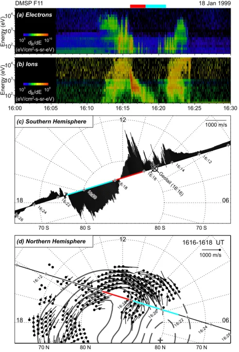
Fig. 11. DMSP F11 (a) electron and (b) ion spectrograms measured between 16:00 and 16:30 UT as the spacecraft traversed the southern

dayside auroral zone. (c) The horizontal drift measured during the DMSP crossing of the Southern Hemisphere, overlaid with the approximate footprint of Geotail at 16:16 UT, when it measured an FTE at the magnetopause. (d) The Northern Hemisphere convection velocities (vectors and velocity streamlines) deduced from all northern hemisphere SuperDARN radars, overlaid with the DMSP track, which has been reflected across magnetic local noon. The red and blue lines above the top panel signify times when cusp/mantle precipitation and virtually no precipitation was measured, respectively, and these correspond to the coloured sections of the satellite trajectory in the lower two panels.

spectrogram is presented in Fig. 11a; as expected, the av-erage energy of the electrons in the cusp is quite small, of the order of 100 eV. The low-energy electron flux dropped suddenly at 16:18:10 UT, the rapid energy dispersion of the cusp ions ceased, and the average ion energy remained low (<200 eV). From 16:18:10 UT to about 16:19:20 UT some very low energy ions were measured, but these may be due to

instrumental effects. At the time the spacecraft was charged −15 V with respect to the plasma, which accelerates ions as they approach the spacecraft, and this acceleration is impor-tant at 30 and 45 eV. The spectrograms are consistent with the spacecraft traversing the cusp through the footprint of newly-reconnected field lines, then passing into the mantle, into the polar cap void and out of the polar cap into the auroral zone at

K. A. McWilliams et al.: Simultaneous FTEs and ionospheric signatures 2195 16:21 UT. The red line at the top of Fig. 11 indicates where

the cusp and then mantle ions were observed, and the blue line indicates the polar cap void.

The horizontal plasma drifts measured by the DMSP drift meter are presented in Fig. 11c. The portions of the tra-jectory where cusp/mantle and then no plasma was detected are coloured red and blue, respectively. As the spacecraft traversed from dawn to dusk, it encountered increasingly variable sunward flow until magnetic local noon when there was a region of antisunward flows. Equatorward of approx-imately 76◦S the flow reversed and was weakly sunward. This pattern of velocities perpendicular to the spacecraft tra-jectory is consistent with an asymmetric twin-cell pattern with the larger convection cell in the prenoon sector and the overall pattern rotated slightly counterclockwise, as expected in the Southern Hemisphere due to the positive IMF By ori-entation at the time.

Unfortunately the SuperDARN radars in the Southern Hemisphere measured very little backscatter at the time. There was, however, excellent coverage in the Northern Hemisphere. The Southern Hemisphere convection patterns for negative IMF By are expected to be very similar to the northern convection pattern for positive IMF By, and vice versa. Reflecting the convection pattern about noon is a rough approximation for determining the convection pattern in the opposite hemisphere. The northern convection pattern, determined from the spherical harmonic fitting technique of Ruohoniemi and Baker (1998), is presented in Fig. 11d, with the DMSP F11 trajectory mirrored across local noon. The component of the SuperDARN vector flows perpendicular to the DMSP trajectory in Fig. 11d is in excellent agreement with the horizontal drifts measured by DMSP in Fig. 11c. The spacecraft measured sunward velocities until just prior to 16:18 UT, as it traversed the dawn auroral zone and passed into the polar cap. In the Northern Hemisphere the convec-tion velocities had a sunward component in the postnoon sec-tor along the mirrored satellite trajecsec-tory, and the poleward velocities were encountered just prior to the 16:16 UT point along the DMSP’s mirrored trajectory. At about 16:21 UT DMSP F11 encountered a reversal of convection from anti-sunward to primarily anti-sunward in the Southern Hemisphere. This coincides with the end of the polar cap traversal deduced from the particle data and occurs at the end of the blue por-tion of the trajectory. The 16:21 UT point along the mirrored trajectory in the Northern Hemisphere is equatorward of the convection reversal boundary of the fitted equipotential con-tours. This is likely primarily an artefact of the convection model used to constrain the fitting procedure, as there are no SuperDARN data points near the 16:21 UT point in the mir-rored trajectory. The convection reversal boundary closer to noon, however, between 9 and 11 MLT, where there is much better data coverage by the radars, is located at the same mag-netic latitude as the 16:21 UT point on the mirrored trajec-tory, where the convection reversal is expected.

At 16:16 UT the Geotail spacecraft measured an FTE on the dawn flank, and its magnetically conjugate position was mapped down to DMSP altitudes using the T96 geomagnetic

Fig. 12. An artistic rendering of the evolution of a flux tube that

reconnected at high southerly latitudes in the prenoon sector and convects past Geotail (◦×G) on the dawn flank.

field model (Tsyganenko and Stern, 1996) in Fig. 11c. The agreement between the Geotail FTE footpoint and the loca-tion of DMSP F11 when it saw the equatorward boundary of the cusp ions is remarkable. These simultaneous and conju-gate measurements of an FTE and a clear energy-dispersed ion signature imply that DMSP F11 passed through the foot-print of active reconnection. The small offset between the Geotail footprint and the onset of energy-dispersed cusp ions at DMSP F11 may be due to several factors, such as inac-curacies in the magnetospheric field line model. The T96 model mapped Geotail’s footprint from just inside the mod-elled magnetopause, when Geotail was situated in the mag-netosheath immediately outside of the actual magnetopause. Another possible factor which may cause an offset is the fi-nite time the ions require to precipitate along the reconnected field lines while they are convecting in the polar cap.

Another feature of data from a spacecraft travelling through the reconnection footprint is a relatively sharp, low energy cutoff for the cusp ions, because particles precipitat-ing along the field with less energy than this cutoff do not have time to reach the spacecraft in the time taken for the field line to convect into the location of the measurement (Lockwood and Smith, 1992). Since these particles have the lowest energy, they have travelled the furthest along the field line and therefore are presumed to originate from the recon-nection site. This low-energy cutoff decreases with increas-ing distance from the footprint of the reconnection site. The Geotail/IMP-8/SuperDARN comparison in Sect. 4.2.2 sug-gested that when FTEs were measured the reconnection site was at high southerly latitudes in the prenoon sector, and the ion energy cutoff may be able to reveal information about the magnetosheath plasma injected at the reconnection site.

A subset of the DMSP ion spectrogram from the south-ern orbit, focusing on the energy-dispersed cusp ions, is presented in Fig. 13. Because of pitch angle scattering, the low energy cutoff can become smeared over a range of en-ergies, so the cutoff energies of the ion distribution function were determined for each energy channel at the point where

Fig. 13. The DMSP F11 ion spectrogram measured between 16:15 and 16:18 UT. The black crosses mark the peak differential energy flux

[eV cm−2s−1sr−1eV−1] in each energy channel, and the white crosses mark where the differential energy flux is 90% or less of the peak value.

Fig. 14. The crosses represent the values of the ion distribution

function [m−6s3] where the differential energy flux is 90% or less of the peak measurement (the white crosses in Fig. 13). The particle energy has been converted to a proton velocity v (E=1₂mpv2). The solid line is a maxwellian fit to the data points. The peak of the fitted maxwellian vpis equal to 340 km s−1.

the differential energy flux dropped to 90% or less of the peak value. This method of determining the low energy ion cut-off has been adopted from Lockwood and Smith (1992). The black crosses in Fig. 13 mark the peak differential energy flux for each energy channel, and the white crosses mark where fluxes drop to 90% or less of peak flux.

The differential energy flux was converted to a velocity distribution function, and the resulting distribution function

of ion cutoffs (Fig. 14) has the form of a truncated drifting maxwellian distribution. This is the field-aligned component of the D-shaped distribution expected in the Earth’s refer-ence frame for a plasma population injected along a convect-ing field line, predicted by Cowley (1982). The peak veloc-ity of the best fit maxwellian distribution (the solid line in Fig. 14) is 340 km s−1, which is 97% of the solar wind ve-locity. The fitted distribution has a temperature of 7×105K, which is about 18 times that of the solar wind ion thermal temperature during this interval. The fitted plasma density is 8 cm−3, which is about 0.8 that in the solar wind. Whilst the errors in such a calculation are vast, the results are all typical of magnetosheath values downstream of the subsolar point (Spreiter and Stahara, 1980). The values derived from the fitted maxwellian are in agreement with the conclusion from the Geotail FTE analysis that the reconnection site is at high latitudes, away from the subsolar point. Acceleration across the reconnection line could produce precipitating energies a factor of two or three larger than the magnetosheath values (Smith et al., 1992), but this would not reduce the injected velocity to subsolar values.

5 Summary

On 18 January 1999 between 14:00 and 18:00 UT, excellent coverage of the directly coupled solar wind, magnetosphere, and ionosphere was achieved. IMP-8 was located immedi-ately upstream of the bow shock, Geotail crossed the dawn-side magnetopause at about 4 MLT, DMSP traversed the southern auroral zone, and SuperDARN covered the entire dayside ionosphere in the Northern Hemisphere. Due to this excellent data set, we were able to develop a very detailed picture of the reconnection process and its effects on the particles and fields of the directly coupled magnetosphere-ionosphere system. This study presents the first simultaneous

K. A. McWilliams et al.: Simultaneous FTEs and ionospheric signatures 2197 independent ionospheric and space-based determinations of

the location of the FTE reconnection site.

The large-scale ionospheric convection velocities re-sponded very directly to the orientation of the upstream IMF. On a smaller scale, transient ionospheric convection velocity enhancements were observed, with a time scale of about ten minutes, throughout the interval. These transient poleward moving radar auroral forms indicate transient reconnection at the magnetopause. The radar transients occurred through-out the 14:00–18:00 UT interval, suggesting that reconnec-tion, in the form of flux transfer events, was occurring on the magnetopause, regardless of the varying orientation of the IMF.

Geotail, located near the equatorial plane on the dawn flank, measured a series of FTE signatures under exclusively northward IMF conditions only when the IMF Bycomponent was strongly positive. The ubiquity of the radar transients in the dayside ionosphere, an indicator of FTE activity, implied that reconnection was continuing during the entire interval, regardless of the IMF orientation. The location of the recon-nection site and the evolution of reconnected flux tubes de-pend primarily on the orientation of the IMF, and the lack of FTEs measured at Geotail during the other IMF orientations was likely due to the spacecraft not being in an appropriate place to view flux tubes reconnected during different IMF conditions.

Localised boundary normal coordinate analysis revealed that the FTE signatures were consistent with a classic flux tube protruding from the magnetopause passing near the spacecraft. These flux tubes were estimated to be roughly 6–7 REacross. The alignment of the magnetosheath field di-rection, from the localised boundary normal analysis, was consistent with reconnected flux tubes connected to the northern ionosphere. Models of the antiparallel merging sites on the magnetopause pointed towards a Southern Hemi-sphere reconnection site in the prenoon sector. Field lines reconnecting at this point with one end passing through the northern ionosphere would have the measured magne-tosheath field direction once they reached the position of Geotail.

The first simultaneous and conjugate measurements of an FTE at the magnetopause and low-altitude DMSP energy-dispersed ions, indicative of the ionospheric footprint of the magnetospheric cusp, were presented. The low-energy cut-off values of the DMSP ion spectrogram were used to recon-struct the plasma distribution injected at the reconnection site itself. This distribution fit extremely well to a truncated drift-ing maxwellian distribution, which is expected for the field-aligned component of the plasma distribution injected at the reconnection site. The characteristics of the injected plasma are consistent with non-subsolar magnetosheath plasma, and this agrees with the high-latitude reconnection site deduced from the Geotail data analysis.

Acknowledgements. K. A. McWilliams is supported by NSERC through PDF-242485-2001 and a Collaborative Research Opportu-nities grant for “Scientific Personnel of the Canadian SuperDARN

Program”. Work by D. G. Sibeck at JHU/APL and NASA/GSFC was supported by NAG5-10479. F. J. Rich is supported by the US Air Force Office of Scientific Research under Task 2311SDA3. The DMSP particle detectors were designed by D. Hardy of AFRL, and data obtained from JHU/APL. We thank D. Hardy, F. Rich, and P. Newell for its use. We would like to thank R. P. Lepping, A. J. Lazarus and the NSSDC for providing IMP-8 data.

Topical Editor T. Pulkkinen thanks two referees for their help in evaluating this paper.

References

Coleman, I. J., Chisham, G., Pinnock, M., and Freeman, M. P.: An ionospheric convection signature of antiparallel reconnection, J. Geophys. Res., 106, 28 995–29 007, 2001.

Cowley, S. W. H.: The causes of convection in the Earth’s magneti-sphere: A review of developments during IMS, Rev. Geophys., 20, 531–565, 1982.

Cowley, S. W. H. and Lockwood, M.: Excitation and decay of so-lar wind-driven flows in the magnetosphere-ionosphere system, Ann. Geophys., 10, 103–115, 1992.

Crooker, N. U.: Dayside merging cusp geometry, J. Geophys. Res., 84, 951–959, 1979.

Davies, J. A., Yeoman, T. K., Rae, I. J., Milan, S. E., Lester, M., Lockwood, M., and McWilliams, A.: Joint CUTLASS Finland and EISCAT VHF radar observations of the ionospheric signa-tures of dayside transient reconnection, Ann. Geophys., 20, 781– 794, 2002.

Dungey, J. W.: Interplanetary magnetic field and the auroral zones, Phys. Rev. Lett., 6, 47–48, 1961.

Elphic, R. C., Lockwood, M., Cowley, S. W. H., and Sandholt, P. E.: Flux transfer events at the magnetopause and in the ionosphere, Geophys. Res. Lett., 17, 2241–2244, 1990.

Farrugia, C. J., Elphic, R. C., Southwood, D. J., and Cowley, S. W. H.: Field and flow perturbations outside the reconnected field line region in flux transfer events: Theory, Planet. Space Sci., 35, 227–240, 1987.

Feldstein, Y. I. and Starkov, G. V.: Dynamic of auroral belt and polar geomagnetic disturbances, Planet. Space Sci., 15, 209–229, 1967.

Goertz, C. K., Nielsen, E., Korth, A., Glassmeier, K.-H., Hal-doupis, C., Hoeg, P., and Hayward, D.: Observations of a pos-sible ground signature of flux transfer events, J. Geophys. Res., 90, 4069–4078, 1985.

Greenwald, R. A., Baker, K. B., Dudeney, J. R., Pinnock, M., Jones, T. B., Thomas, E. C., Villain, J.-P., Cerisier, J.-C., Senior, C., Hanuise, C., Hunsucker, R. D., Sofko, G., Koehler, J., Nielsen, E., Pellinen, R., and Walker, A. D. M.: DARN/SuperDARN: a gloval view of the dynamics of high-latitude convection, Space Sci. Rev., 71, 761–796, 1995.

Haerendel, G., Paschmann, G., Sckopke, N., Rosenbauer, H., and Hedgecock, P. C.: The frontside boundary layer of the magne-tosphere and the problem of reconnection, J. Geophys. Res., 83, 3195–3216, 1978.

Hardy, D. A., Schmitt, L. K., Gussenhoven, F. J., Yeh, H. C., Schumaker, T. L., Hube, A., and Pantazis, J.: Precipitating electron and ion detectors SSJ/4 for the block 5D/flights 6–10 DMSP satellites, Report AFGL-TR-84-0317, Air Force Geo-physics Laboratory, Hanscom Air Force Base, Mass., USA, 1985.