Aliphatic and aromatic hydrocarbons in comet 67P/Churyumov-Gerasimenko seen by ROSINA

HAL Id: insu-02293706

https://hal-insu.archives-ouvertes.fr/insu-02293706

Submitted on 10 Nov 2020

HAL is a multi-disciplinary open access

archive for the deposit and dissemination of

sci-entific research documents, whether they are

pub-lished or not. The documents may come from

teaching and research institutions in France or

abroad, or from public or private research centers.

L’archive ouverte pluridisciplinaire HAL, est

destinée au dépôt et à la diffusion de documents

scientifiques de niveau recherche, publiés ou non,

émanant des établissements d’enseignement et de

recherche français ou étrangers, des laboratoires

publics ou privés.

67P/Churyumov-Gerasimenko seen by ROSINA

M. Schuhmann, Kathrin Altwegg, Hans Balsiger, Jean-Jacques Berthelier,

Johan de Keyser, Björn Fiethe, S. A. Fuselier, S. Gasc, T.I. Gombosi, N.

Hänni, et al.

To cite this version:

M. Schuhmann, Kathrin Altwegg, Hans Balsiger, Jean-Jacques Berthelier, Johan de Keyser, et al..

Aliphatic and aromatic hydrocarbons in comet 67P/Churyumov-Gerasimenko seen by ROSINA.

Astronomy and Astrophysics - A&A, EDP Sciences, 2019, 630, A31 (11 p.).

�10.1051/0004-6361/201834666�. �insu-02293706�

&

Astrophysics

Special issue

© ESO 2019

Rosetta mission full comet phase results

Aliphatic and aromatic hydrocarbons in comet

67P/Churyumov-Gerasimenko seen by ROSINA

M. Schuhmann

_{, K. Altwegg}

_{, H. Balsiger}

_{, J.-J. Berthelier}

_{, J. De Keyser}

_{, B. Fiethe}

_,

S. A. Fuselier

_{, S. Gasc}

_{, T. I. Gombosi}

_{, N. Hänni}

_{, M. Rubin}

_{, C.-Y. Tzou}

_{, and S. F. Wampfler}

1_{Space Research and Planetary Sciences, University of Bern, Bern, Switzerland}

e-mail: markus.schuhmann@space.unibe.ch

2 _{Center for Space and Habitability, University of Bern, Gesellschaftsstrasse 6, Bern, Switzerland} 3_{Institut Pierre Simon Laplace, CNRS, Université Pierre et Marie Curie, Paris, France}

4_{Koninklijk Belgisch Instituut voor Ruimte–Aeronomie, Institut Royal Belge d’Aéronomie Spatiale, Avenue Circulaire 3,}

Uccle, Belgium

5_{Institut für Datentechnik und Kommunikationsnetze, TU Braunschweig, Braunschweig, Germany} 6_{Space Science Directorate, Southwest Research Institute, San Antonio, Texas, USA}

7_{University of Texas at San Antonio, San Antonio, Texas, USA}

8_{Department of Climate and Space Sciences and Engineering, University of Michigan, Ann Arbor, USA}

Received 16 November 2018 / Accepted 10 April 2019

ABSTRACT

Context. Unlike all previous cometary space missions, the Rosetta spacecraft accompanied its target, comet

67P/Churyumov-Gerasimenko, for more than two years on its way around the Sun. Thereby, an unexpected diversity and complexity of the chemical composition was revealed.

Aims. Our first step of decrypting the exact chemical composition of the gaseous phase is the identifying and quantifying the bulk

composition of the pure aromatic and aliphatic hydrocarbons.

Methods. For this study, data from ROSINA–Double Focusing Mass Spectrometer (DFMS) onboard the Rosetta spacecraft and the

laboratory twin model were used. A joint campaign of laboratory calibration measurements and space data analysis was performed to derive the hydrocarbon bulk composition for the post-inbound equinox period at 1.52 AU in May 2015. Furthermore, several other mis-sion phases were investigated to determine the dependencies of season, location, and heliocentric distance on the relative abundances of hydrocarbons.

Results. It is shown that the bulk composition of the gaseous phase includes a high number of aliphatic compounds such as methane,

ethane, and propane, as well as the aromatic compounds benzene and toluene. Butane and pentane were successfully identified in mea-surements at closer distance to the comet in May 2016. Furthermore, the presence of hexane and heptane in the coma is confirmed on rare occasions during the mission. Their presence in DFMS space data appears to be linked to days or periods of high dust activity. In addition to the saturated aliphatic and aromatic compounds, a high number of remaining unsaturated species is present, which cannot be explained by fragmentation of saturated species or contribution from other organic molecules in addition to pure hydrocarbons. This indicates the existence of unsaturated aliphatic and aromatic hydrocarbon molecules in the coma of comet 67P.

Key words. comets: general – comets: individual: 67P/Churyumov-Gerasimenko

1. Introduction

The European Space Agency’s Rosetta mission has marked a cornerstone in cometary space science. Unlike all previous cometary space missions, Rosetta accompanied its target, comet 67P/Churyumov-Gerasimenko (hereafter 67P) for an extended

time period of more than two years (Glassmeier et al. 2007).

Furthermore, the first soft landing on a comet was performed, and data from the surface were collected by the Rosetta lan-der Philae. A suite of 11 instruments on the orbiter module and another 10 instruments on the lander allowed an in depth inves-tigation of many physical and chemical properties of the nucleus

and coma (Bibring et al. 2015;Taylor et al. 2015). This detailed

investigation was justified because comets contain a unique well-preserved reservoir of the material that formed our solar system. Of special interest are certainly the organics found in comets because they not only present a fingerprint of the chemical and

physical conditions before and during solar system formation, but may also help us to constrain the delivery of organic matter by comets on the early Earth. More than 30 yr ago, the flyby of the Giotto spacecraft at comet Halley revealed complex organics

up to mass 100 u/e (Mitchell et al. 1987) in a cometary coma.

However, the mass resolution was not sufficient to identify the molecules. The only organics that have clearly been identified in cometary coma before Rosetta are low-mass molecules seen

with remote sensing from the ground (Bockelée-Morvan et al.

2000; Mumma & Charnley 2011). It became apparent already very early in the Rosetta mission that organics play an impor-tant role for 67P not only in the volatile part of the coma, but

also in the refractories (Fray et al. 2016).Capaccioni et al.(2015)

reported that the dark surface and low albedo of 67P are compat-ible with a polyaromatic carbonaceous component mixed with

opaque minerals, while Quirico et al.(2016) reported carbon–

spectrum. Many of the organics known to exist in cometary coma from remote sensing could be detected in the coma of 67P

already beyond 3 au (Le Roy et al. 2015). Organic compounds on

comet 67P have been observed by various instruments, including the lander mass spectrometer Cometary Sampling and

Compo-sition Experiment (COSAC;Goesmann et al. 2015) and Ptolemy

(Wright et al. 2015). A comparison of the COSAC, Ptolemy, and

ROSINA mass spectra analysis is provided by Altwegg et al.

(2017), who listed the coherence and differences in

interpreta-tion of the observed organic composiinterpreta-tion. The unexpected high complexity and diversity of detected organic molecules includ-ing CH-, COOH-, HCN-, CHS-, CNOH-, and HCO-bearinclud-ing compounds makes analysis difficult and time consuming, and demands significant laboratory work. In the present study a calibration campaign was performed on several aliphatic and aromatic hydrcarbons to obtain their fragmentation pattern and the detector sensitivity for ROSINA–DFMS mass spectrome-ters. Based on the calibration results and data from the National Institute of Standards and Technology (NIST), an identification campaign on hydrocarbons in the coma of comet 67P was per-formed. Furthermore, the relative abundances were calulated for various mission phases and compared to other studies.

2. Methods and observations

ROSINA, the Rosetta Orbiter Spectrometer for Neutral and Ion Analysis, consists of three different instruments: the Cometary Pressure Sensor (COPS) and two mass spectrometers, the Reflectron-type Time-Of-Flight (RTOF) and the Double

Focus-ing Mass Spectrometer DFMS (Balsiger et al. 2007). Unlike

other mass spectrometers on the lander Philae, ROSINA had

a much longer investigation time (Altwegg et al. 2017). From

the arrival at the comet in 2014 until the end of mission on 30 September, 2016, ROSINA measurements where performed in different settings. These measurements support the scientific goal for ROSINA of long-term observation of the cometary coma during the crucial stages of the comet’s orbital path, including the inbound and outbound equinoxes and perihelion. 2.1. DFMS operation and settings

The presented work is based on data collected with ROSINA–

DFMS built in Mattauch–Herzog configuration (Mattauch &

Herzog 1934). DFMS allowed operation with filament emission of either 2, 20, or 200 µA and could be operated in low-resolution and high-low-resolution mode (where the zoom factor was 6.4 times higher than in low-resolution mode). DFMS used electron impact ionization with an electron energy of 45 eV to ionize incoming neutral gas, which is different from the 70 eV

standard in mass spectrometry (Balsiger et al. 2007). After

ion-ization, ion optics allowed only ions with a specific mass/charge ratio to pass through the analyzer section. This section contained both an electrostatic and a magnetic analyzer. For ion detec-tion, a microchannel plate (MCP) with a position-sensitive linear anode (Linear Electron Detector Array, LEDA) with 512 pixels

was used (Nevejans et al. 2002). The LEDA consisted of two

rows for redundancy reasons (designated rows A and B in the spectra). A constant voltage of 200 V was applied at the back-side of the detector. The voltage across MCP, which determined the detector gain, was adjusted in 16 steps that each amplified the signal by roughly a factor 2.6. The DFMS measurement range was from integer mass/charge 13 to 180 u/e. Nominally, mass/charge 13–100 u/e were scanned within roughly 45 min, including 10 s settling time after applying the voltages and v20 s

of integration. Lower and higher masses could not be detected because of limitations on the acceleration voltage, detection effi-ciencies, and the low abundance of these volatiles in the coma. As the acceleration voltage decreased toward higher masses, an additional post-acceleration voltage was applied for measure-ments of mass/charge ratios 70 u/e and higher to maintain the detector sensitivity. DFMS had a mass resolution of 3000 at 1% peak height at mass/charge 28 u/e. For this study, a filament emission current of 200 µA and high-resolution mode was used. The main investigation period covers May and early June 2015 and was selected for several reasons: (I) the heliocentric distance of comet 67P of 1.5 au allowed measuring the abundances before

the coma became highly dynamic due to outbursts (Vincent et al.

2016).Calmonte et al.(2016) found this period to be the most representative to estimate nucleus bulk abundances. First, the Rosetta spacecraft was located over the active southern summer hemisphere and on the sunward side of the nucleus down to a

phase angle of almost 60◦_{. Thus, it provides good conditions}

for identifying and quantifying the saturated aliphatic and aro-matic hydrocarbon abundances inside the nucleus of comet 67P. The disadvantage was that the spacecraft was relatively far from the nucleus (v200–300 km). Furthermore, measurements from May 2016, when the spacecraft was very close to the nucleus, but the comet was already far from the Sun (2.95 au), were ana-lyzed and compared to the investigation period in May and June 2015. Because the analysis of the event on 5 September, 2016, (Altwegg et al. 2017), with data obtained under conditions that significantly vary from both May 2015 and 2016, indicated a large number of hydrocarbons at high dust activity, this study also includes an analysis of spectra from March 2015 and 10 July, 2015, where ROSINA COPS showed signatures of semi-volatile grains impacting and evaporating in or close to COPS (see Altwegg et al. 2017).

2.2. Data treatment

For DFMS, the two spectra for rows A and B contain a small range of mass/charge around the integer mass/charge. These spectra provide the raw counts in each of the 512 LEDA pix-els. To correctly identify and quantify the peak, several steps are required: (I) the offset of the signal had to be removed. (II) The detector gain had to be corrected for each pixel. (III) The num-ber of ions had to be calculated from the ADC (raw) counts. (IV) A mass scale had to be applied for each spectrum. Because the magnetic field of the permanent magnet in DFMS is tem-perature dependent, the mass scale had to be adjusted in order to obtain consistent mass spectra. Application of the mass scale is more difficult in spectra of high integer mass because DFMS spectra generally show lower peak intensities and mass resolu-tion. To identify CH-fragments in spectra with high integer mass, the high number of hydrogen atoms helps to identify

hydrocar-bons because of the high mass defect of hydrogen. Schläppi

et al.(2010) reported a high molecular adsorption potential on the Rosetta orbiter surface and solar panels. Thus, any change in lateral angle between spacecraft and Sun during maneuvers can lead to significant desorption and outgassing. For this study, we therefore only took DFMS measurements without time overlap to spacecraft maneuvers or thruster firings into account. How-ever, low levels of outgassing always occurred even without

maneuvers (Schläppi et al. 2010), but they can be neglected in

the chosen investigation period because of the high molecular densities in the coma close to perihelion.

DFMS peaks are approximated by double Gaussians (Rubin

represent the peak shape. However, in this study the number of ions is derived directly by summing all incident ions of the LEDA pixels under the peak without fitting any Gaussians. In addition to the uncertainties based on the fitting method, fur-ther uncertainties for in species-dependent sensitivity and the effects of post-acceleration of molecules of mass/charge 70 u/e and higher must be taken into account. Further information is

found inLe Roy et al.(2015),Calmonte et al.(2016), andRubin

et al.(2015).

2.3. DFMS calibration and fragmentation

The ROSINA instruments were calibrated at the Bernese calibra-tion facility called CAlibracalibra-tion SYstem for the Mass spectrom-eter Instrument ROSINA (CASYMIR), which was developed for testing and calibration under space-equivalent low-density

conditions (Westermann et al. 2001). It allows operation at

10−10_–10−6_{mbar and can be used in a static background mode in}

molecular-beam mode to simulate the outflow of cometary gases (Graf et al. 2004). To calibrate aliphatic and aromatic hydro-carbons in the DFMS laboratory model, the compounds were transferred from liquid into gas phase by heating the sample tube

to 323 K at low pressure in the range of 10−6_{mbar. The gas was}

introduced through a leak valve into CASYMIR/DFMS where measurements were performed. This procedure was repeated at

three different pressure levels p = 3 × 10−9_{mbar, 2 × 10}−8_mbar,

and 1 × 10−7_{mbar to cover a maximum density range. In}

addi-tion, background measurements were performed and subtracted from the actual measurements. Calibration of DFMS on aliphatic and aromatic hydrocarbons was necessary for several reasons: (I) in addition to charging neutral molecules positively, the elec-tron impact ionization used in mass spectrometry also breaks molecular chains and thus leads to a detection of the fragments and the parent molecule in the mass spectra. This process is called fragmentation and depends on the electron energy used for ionization. It results in a fragmentation pattern with species-dependent abundances, which can be used to identify or exclude species in mass spectra. However, the pattern also depends on the molecular structure of the ionized species and thus can be used to distinguish isomers such as n-butane and isobutane. Com-pounds such as pentane, heptane, and octane with higher masses are significantly affected, leading to complex fragmentation pat-terns. (II) The DFMS sensitivity on a compound is calculated from the detected number of ions. Therefore pressure condi-tions must be stable over the measurement period. This can be especially challenging for volatile organic compounds. Thus, a thermal valve-control system was used to stabilize the partial pressure of the component in CASYMIR during the calibration cycle. The DFMS calibration campaign included the saturated aliphatic compounds up to octane (integer mass/charge 114 u/e). The calibration campaign on butane, pentane, hexane, heptane, and octane was made with unbranched molecule version (e.g., n-pentane), while for methane, ethane, and propane, no differ-entiation in terms of structural isomerism appears. For benzene, the DFMS calibration was not performed because the compound is highly toxic in the gas phase. In addition to the fragmenta-tion, the DFMS calibration campaigns were performed to derive the sensitivity of DFMS for measured compounds. Hereby the ratio of the ion current to the molecular density was derived for each pressure level. The slope between ion current and density for each of the three pressure levels is the sensitivity factor. As an alternative, when no calibration could be obtained, the sen-sitivity was calculated based on the ionization cross-section of the molecule. The sensitivities used in this study can be found

20 30 40 50 60 70 20 40 60 80 100 DFMS relative Abundance [%] m/z [u/e] NIST

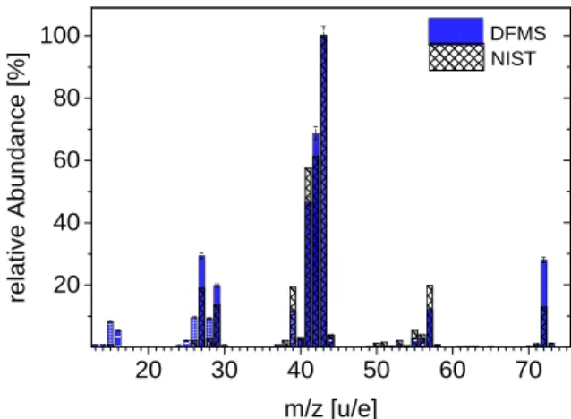
Fig. 1.DFMS fragmentation pattern of n-pentane. The plot shows the fragmentation of pentane caused by DFMS 45 eV ionization energy. The amount of fragmentation is relative to the most abundant frag-ment C3H7. In comparison, we show the NIST fragmentation patttern

for pentane using 70 eV ionization energy.

in AppendixA. Relative abundances were calculated based on

DFMS laboratory and space data, taking into account the sensi-tivity, the fragmentation pattern, and the number of ions (from DFMS space data) The procedure equals the procedure used by Gasc et al.(2017) for ROSINA–RTOF (Eqs. (13) and (14)) and can equally be applied for DFMS even though the DFMS sensitivity depends on more parameters, but DFMS specific instrumental factors are cancelled out in the equation.

3. Results

3.1. Fragmentation

Results for the calibration campaign for saturated aliphatic com-pounds are presented in this section. The fragmentation pattern

of pentane is shown in Fig.1. More fragmentation patterns are

found in the appendix. AppendixBshows that unbranched

alka-nes of higher masses have complex, but similar fragmentation patterns, illustrating a broad range of fragments with slightly different relative abundances. For saturated aliphatic compounds higher than ethane, the ionized parent molecule is not the high-est peak. Moreover, unsaturated fragments may show reactive behavior, leading to molecular recombination processes in the ion source. However, calibration measurements show that low numbers of saturated fragments are present in the fragmentation pattern even after the background is removed. This demonstrates that rearrangement processes may occur and lead to formation of

saturated molecules with very minor abundance (see Fig.1).

When we compare the results of the DFMS calibration cam-paign to results reported in the literature, differences between DFMS abundances and databases like that of NIST are

appar-ent (Fig.1). This confirmsAltwegg et al.(2017), who showed

that the ionization energy of 45 eV used by DFMS leads to a change in the fragmentation pattern and in the remaining number of the ionized parents compared to NIST. Furthermore, DFMS sensitivities and post-acceleration lead to additional differences in comparison to NIST.

3.2. Application to DFMS space data

As reported in previous studies such as Le Roy et al.(2015),

the fragmentation of all relevant species must be taken into account to successfully identify and tentatively quantify them.

15.96 15.98 16.00 16.02 16.04 0.1 1 10 100 1000 10000 100000

Ions per 20 sec

m/z [u/e] CH₄ NH₂ 15 NH S++ O

Fig. 2.Methane [CH4]. DFMS space data show methane in May 2015.

Thus, to identify a species in the DFMS space data, not only the ionized parent molecule, but also all main fragments must be present in the spectra. This leads to a certain complexity in the analysis because fragments originate from multiple species. To correctly identify a molecule as a parent molecule, several crite-ria need to be fulfilled: (I) the parent molecule is identified in the mass spectrum. (II) All main fragments are found in the data. (III) Contribution from other species cannot explain the abun-dances of the suggested parent and its fragments. Furthermore, the wide range of hydrocarbon structures and potential con-tributors such as alcohols increase the difficulty of correctly identifying and quantifying aliphatic and aromatic hydrocarbons in DFMS space data.

3.2.1. Identification and quantification campaign

DFMS space data from the May 2015 inbound post-equinox period indicate several aliphatic and aromatic hydrocarbons.

Methane [CH4] (Fig. 2), ethane [C2H6] (Fig. 3), and propane

[C3H8] (Fig.4) were confirmed. Furthermore, the aromatic

com-pounds benzene [C6H6] (Fig.7) and toluene [C7H8] (Fig.9) were

confirmed. Toluene has a particular impact on the identification and quantification attempt of saturated hydrocarbon compounds because the fragmentation of toluene can lead to the formation

of small numbers of saturated compounds such as [CH4] and

[C2H6]. However, because the produced fluxes from the comet

decrease with increasing mass and complexity of the molecules, this contribution remains small.

Unsaturated CH-species at 50–57 u/e further indicate butane

[C4H10], although the parent molecule is below the detection

limit in this period. Pentane or any higher saturated aliphatic compound were not detected either in May 2015. However,

butane (Fig.5) and pentane [C5H12] (Fig.6) were confirmed in

May 2016, where DFMS measurements were performed much closer to the cometary nucleus and densities were significantly higher. Further investigation also showed hexane in May 2016

(Fig. 8), but only as rare events because it was not found

during most measurement days. Their count rates above back-ground were limited to certain measurements on single days (e.g., 6 May 2016). These results confirm the overall picture, as

hexane [C6H14] and heptane [C7H16] (Fig.10) were not found

in May 2015, but were seen under specific conditions as rare events in July 2015. The appearance of heptane and hexane is likely related to dust-rich events. It therefore appears that while lower mass hydrocarbons are found in cometary ices and desorb

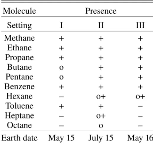
Table 1. Hydrocarbons detected by ROSINA in the coma of comet 67P in May 2015, July 2015, and May 2016.

Molecule Presence Setting I II III Methane + + + Ethane + + + Propane + + + Butane o + + Pentane o + + Benzene + + + Hexane – o+ o+ Toluene + + – Heptane – o+ – Octane – o –

Earth date May 15 July 15 May 16

Notes. I: post-equinox period at 1.52 au. II: dust impact period close to perihelion at 1.27 au. III: close to outbound at 2.95 au. (+): species is present: parent and fragments are visible. (o+): presence of species at single events only. (o): presence of fragments, parent not detected. (–): species is not identified in this period. Detection limit is estimated to be 10 ions. 29.96 29.98 30.00 30.02 30.04 30.06 0.1 1 10 100 1000

Ions per 20 sec

m/z [u/e]

NO H₂CO

H₄CN C₂H₆

Fig. 3.Ethane [C2H6]. DFMS space data show ethane in May 2015.

with water, higher mass hydrocarbons are tied to dust grains and

desorb from hot dust grains in the coma (Lien 1990).

Table 1 lists an overview of the detected hydrocarbons in

the different investigated mission phases. A plus means that a species is clearly present as parent and all main fragments are visible. An empty circle means that the data indicate fragments, but the parent could not be found or detected unequivocally in this period. This might be due to limited resolution, back-ground noise, or the peak detection limit, which is estimated to be around 10 ions combined during the 20 s integration time. A large comet-spacecraft separation also led to low peak inten-sities. A minus indicates that a species is not identified in this period. An empty circle with a plus means that a species was confirmed for single events only in this mission phase. These events appear to correlate with dust activity.

In general, a decrease in peak intensity toward higher masses

is seen (see Figs. 2–10). This trend is confirmed also for

May 2016 at small spacecraft-comet distances (with the excep-tion of ethane). Following this trend, the parent peaks of butane and pentane in May 2015 are probably below the detection limit, and might not be found for this reason, particularly because

43.96 44.00 44.04 44.08 0.1 1 10 100 1000 10000

Ions per 20 sec

m/z [u/e] CS CO 2 CNOH 2 C₂OH₄ C₃H₈ C₂NH₆

Fig. 4.Propane [C3H8]. DFMS space data show propane in May 2015.

58.02 58.04 58.06 58.08 58.10 58.12 0.1 1 10 100 1000

Ions per 20 sec

m/z [u/e]

C₃OH₆

C₄H₁₀

Fig. 5.Butane [C4H10]. DFMS space data show butane in May 2016.

72.04 72.08 72.12 72.16 0.1

1 10 100

Ions per 20 sec

C₄OH₈

C₅H₁₂

m/z [u/e]

Fig. 6.Pentane [C5H12]. DFMS space data show pentane in May 2016.

the DFMS fragmentation pattern for aliphatic compounds gen-erally showed low abundances for the parent molecules. This seems more reasonable than the total absence of both species in the cometary bulk, especially as spectra in May 2016, at much shorter distance to the comet, showed both species.

After the hydrocarbons were successful identified, including a quantification of the compounds, the relative abundances were

derived according toGasc et al.(2017). In this study, abundances

were calculated relative to methane, which was the dominant hydrocarbon in the main investigation phase in May 2015. Furthermore, the abundances of the CH-species were calcu-lated relative to water. For a better understanding of the impact

77.92 77.96 78.00 78.04 78.08 0.1

1 10 100

Ions per 20 sec

C32 S34 S C 6H6 m/z [u/e]

Fig. 7.Benzene [C6H6]. DFMS space data show benzene in May 2015.

85.9 86.0 86.1 86.2 0.1 1 10 100 86 Kr C6H14

Ions per 20 sec

m/z [u/e]

Fig. 8.Hexane [C6H14]. DFMS space data show hexane in May 2016.

91.0 91.2 91.4 91.6 91.8 92.0 1 2 3 4 5 6 7 8

Ions per 20 sec

C₇H₇

C₇H₈

m/z [u/e]

Fig. 9.Toluene [C7H8]. DFMS space data show toluene in May 2015.

of heliocentric distance, the same calculations were also per-formed for May 2016 at 2.95 au. The results of both observation

campaigns are provided in Table2. In addition, in Fig.11the

abundances relative to methane are shown, and in Fig. 12 the

abundances relative to water are shown.

The abundances of the aliphatic compounds relative to both water and methane decrease with higher mass. However, as

shown in Figs.11and12, this trend occurs only for May 2015,

but for abundances relative to both water and methane. The

pat-tern for CH4 and water is very similar in each of the periods

in the two figures. However, a comparison of abundances in May 2015 and May 2016 indicates a significant change in the

100.00 100.05 100.10 100.15 1 2 3 4 5 6 7 8 C₅O₂H₈ C2N5H6

Ions per 20 sec

m/z [u/e]

C₇H₁₆

Fig. 10.Heptane [C7H16]. DFMS space data show heptane in July 2015.

Table 2. Relative abundances.

May 2015

Species Abundance

relative to Methane [CH4] Water [H2O]

Methane (1.00 ± 0.00) × 10+0 _{(3.43 ± 0.68) × 10}−3

Ethane (8.51 ± 1.70) × 10−1 _{(2.92 ± 0.58) × 10}−3

Propane (5.25 ± 1.05) × 10−2 _{(1.80 ± 0.36) × 10}−4

Butane Not detected(∗) _{Not detected}(∗)

Pentane Not detected(∗) _{Not detected}(∗)

Benzene (2.02 ± 0.41) × 10−3 _{(6.94 ± 1.39) × 10}−6

Toluene (1.80 ± 0.36) × 10−2 _{(6.16 ± 1.23) × 10}−5

May 2016

Species Abundance

relative to Methane [CH4] Water [H2O]

Methane (1.00 ± 0.00) × 10+0 _{(6.48 ± 1.30) × 10}−2 Ethane (7.92 ± 1.58) × 10+0 _{(5.13 ± 1.03) × 10}−1 Propane (4.24 ± 0.85) × 10−1 _{(2.75 ± 0.55) × 10}−2 Butane (8.15 ± 1.63) × 10−2 _{(5.28 ± 1.06) × 10}−3 Pentane (7.02 ± 1.40) × 10−2 _{(4.55 ± 0.91) × 10}−3 Benzene (1.21 ± 0.24) × 10−2 _{(7.81 ± 1.56) × 10}−4

Toluene Not detected(∗) _{Not detected}(∗)

Notes.(∗)_{Detection limit is estimated to be 10 ions.}

relative abundances. In May 2016, C2H6 increased relative to

CH4. This ratio differs significantly from the abundances that

were calculated for May 2015. Furthermore, the C3H8abundance

increased as well, apparently following the trend of C2H6. In

general, the relative abundances with respect to H2O increase

in May 2016 as a significant drop in the water production rate

occurs (Laeuter et al. 2019).

In both cases, measurements were made while the spacecraft was above the southern hemisphere. In 2015, this hemisphere was the very active summer hemisphere, while in 2016, the

subsolar latitude was at v5◦ _{north. Figure 11 shows that the}

hydrocarbons heavier than methane appear to be enriched in 2016 compared to 2015. This is surprising considering the already large distance to the Sun in 2016 and that the volatility

of CH4is higher than that of C2H6.

In contrast to the aliphatic compounds, the aromatic species do not follow the general trend of depletion toward higher mass.

Figures11and12show that the relative abundances of toluene

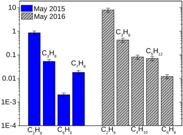
1 E - 4 1 E - 3 0 . 0 1 0 . 1 1 1 0 C ₇H ₈ C 5H 1 2 C 4H 1 0 C 6H 6 C ₆H ₆ C ₃H ₈ C 3H 8 C ₂H ₆ C ₂H ₆ M a y 2 0 1 5 M a y 2 0 1 6

Fig. 11. Abundance of CH-species relative to methane [CH4] with

estimated bulk abundance in May 2015. Heliocentric distances in May 2015: 1.52 au and in May 2016: 2.95 au.

1 E - 7 1 E - 6 1 E - 5 1 E - 4 1 E - 3 0 . 0 1 0 . 1 1 C ₇H ₈ C 6H 6 C ₃H ₈ C ₂H ₆ C H ₄ C H 4 C ₂H ₆ C ₃H ₈ C ₄H _{1 0} C 5H 1 2 C ₆H ₆ M a y 2 0 1 5 M a y 2 0 1 6

Fig. 12. Abundance of CH-species relative to water [H2O] with

estimated bulk abundance in May 2015. Heliocentric distances in May 2015: 1.52 au, and in May 2016: 2.95 au.

are higher than those of benzene. This seems to be in contrast

to the peak intensities of benzene (Fig. 7), which are higher

than those of toluene (Fig. 9), but it can be explained by the

lower DFMS sensitivity for toluene, which has to be taken into account when relative densities inside the DFMS ion source are derived from the measured detector signals. Also in contrast to the aliphatic compounds, the abundance of benzene relative to

CH4did not change significantly from May 2015 to May 2016.

The evolution of the relative abundance of benzene and toluene between the two periods would be very interesting, but could not be investigated as toluene could no longer be found regularly in May 2016.

3.2.2. Impact of cometary and observational parameters In addition to the identification and quantification campaign, we further investigated the impact of cometary rotation and sub-spacecraft latitude and longitude on the measured abun-dances. First, a comparison of measurements on several days in May 2015 was performed to determine whether the relative

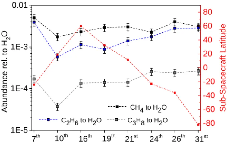
1E-5 1E-4 1E-3 0.01 31st 26th 24th 21st 19th 16th 10th _{CH4 to H2O} C2H6 to H2O C3H8 to H2O 7th -80 -60 -40 -20 0 20 40 60 80 Abundance rel. to H 2 O Sub-Spacecraft Latitude

Fig. 13.Relative abundances in May 2015. We show the abundance of CH4 (black), C2H6 (blue), and C3H8 (gray) relative to water on

sev-eral measurement days in May 2015. We also show the sub-spacecraft latitude at the time of measurement (red).

abundance of the most dominant hydrocarbon species to water changes over the main investigation period and if any trends could be observed. Therefore, DFMS space data on various days were selected and the relative abundances of methane, ethane, and propane to water were calculated. The results are

given in Fig.13. Over the whole month, thus independent from

sub-spacecraft latitude, the methane-to-water ratio remains the highest. However, results also show that there is a change in the relative abundance between methane and water, especially around 10 May. This trend is followed by the ethane-to-water ratio and by the propane-to-water ratio, suggesting external influence as the driving force here. No significant change in the distance comet-spacecraft occurred during the measurement period. However, for further investigation, the sub-spacecraft

lat-itude at the time of measurement was added to the plot. Figure13

shows that no clear correlation with sub-spacecraft latitude can be found for any of the abundance evolution lines.

In addition, we investigated the abundance over several hours, representing a cometary rotation period, in DFMS data taken on 1 and 2 June 2015, when the coma was dominated

by H2O. The measurements were taken over the southern

hemi-sphere at a sub-spacecraft latitude of −70 to 65◦_{. To show the}

evolution of the dominant hydrocarbon peaks over a cometary rotation, with changing sub-spacecraft longitude and latitude, we plot the peak intensities of methane and ethane relative to oxy-gen. For a detailed picture, every DMFS measurement in one measurement cycle consisting of 12 measurements (each sep-arated by 45 min) was analyzed to derive the variation of the intensities over one cometary rotation. The results are shown in

Fig. 14. In addition, the elapsed time in minutes and the

lati-tude and longilati-tude of the sub-spacecraft point in the comet-fixed frame are shown. Between measurements of mass/charge 16 u/e, oxygen and methane, and mass/charge 30 u/e, ethane, a time difference of 8 min occurs, which is neglected for this study. The first analyzed measurement was taken at 209.6 km distance from the comet. This value increases slightly to 216.1 km for the last analyzed measurement. The sub-spacecraft latitude is shown

in the plot; it changes from −70.6◦ _{at the first measurement to}

−65.7◦_{at the last measurement, while the sub-spacecraft}

longi-tude changes significantly from −78.3◦ _{to −41.3}◦_{. As shown in}

Fig.14, the ratio of methane relative to oxygen does not change

much during the rotational period, and all changes are within the error bars. Similarly, for ethane to oxygen over a comet rotation,

0 100 200 300 400 500 1E-3

0.01 0.1

CH₄ to O C₂H₆ to O

Relative Intensity [Peakarea]

Time [min] -180 -160 -140 -120 -100 -80 -60 -40 -20 0 20 40 60 80 100 120 140 160 180 Longitude [°] -90 -80 -70 -60 -50 -40 -30 -20 -10 0 10 20 30 40 50 60 70 80 90 Latitude [°]

Fig. 14.Evolution of hydrocarbon peaks over a cometary rotation. The plot shows the evolution for methane and ethane relative to the oxygen peak over the rotation duration of the comet (error bars are 1σ). The height of the bar represents the relative peak size. We also plot the lat-itude (orange) and longlat-itude (blue) below the spacecraft. Spectra were taken every 45 min with a time difference of 8 min between mass 16 u/e, oxygen, and methane, and mass 30 u/e, ethane.

all changes occur within 1σ for methane and 2σ for ethane and seem independent of latitude and longitude. Thus, no trend of evolution of methane and ethane over a cometary rotation is observed.

3.2.3. Unsaturated hydrocarbons and isomerism

It is difficult to differentiate isomers because no difference in mass/charge for the parent can be observed for different iso-mers. However, another method for distinguishing is the different fragmentation patterns because the branching of molecules also affects fragmentation. When the fragmentation pattern for n- and iso-structured aliphatic compounds is compared, small differ-ences in the relative abundances occur: when we compared the

fragmentation results of NIST (Stein 2018) for n-pentane and

iso-pentane, we obtained higher relative abundances for some fragments (such as at mass 27, 29, 41, 42, and 57 u/e) by fragmen-tation of the branched version. In addition, higher abundances

for CH3(15 u/e) are detected. However, in summary, the

differ-ence in abundance is rather small and appears to occur mostly on masses where unsaturated CH-species are present in the DFMS data from the comet. Thus a differentiation between the different isomers is not possible for the investigated periods. Neverthe-less, isomerism is probably occurring, most likely in the form of single-branched aliphatic compounds. However, as pointed out above, isomerism does not affect any aliphatic compounds of masses lower than butane.

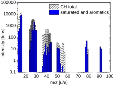
The DFMS space data show unsaturated hydrocarbons in all investigated periods. The observed abundances follow the trend of the saturated molecules and decrease toward higher masses. After accounting for all saturated hydrocarbon parent molecules and their fragments, many CH-bearing compounds remain in the

spectrum (Fig.15). These can only be explained by species

con-taining double or triple bonds or being unsaturated fragments. In addition to the investigated aliphatic and aromatic species, the potential presence of cycloalkanes is discussed here. Cyclo-propane and cyclobutane are indicated by the high number of

unsaturated species and C3H6and C4H8in May 2015, while the

aliphatic parent C4H10was not detected in the same period.

Figure15shows that the total ion signal of saturated aliphatic

2 0 3 0 4 0 5 0 6 0 7 0 8 0 9 0 1 0 0 0 . 1 1 1 0 1 0 0 1 0 0 0 1 0 0 0 0 1 0 0 0 0 0 In te n s it y [ Io n s ] m / z [ u / e ] C H t o t a l s a t u r a t e d a n d a r o m a t i c s

Fig. 15. Total number of CH-species. The plot shows the measured

intensities for pure hydrocarbons up to mass/charge 100 u/e. In blue we show the number that can be explained by the identified saturated aliphatic and aromatic species as well as their fragments.

20 30 40 50 60 70 80 90 100 0.1 1 10 100 1000 10000 100000 Intensity [Ions] m/z [u/e]

remaing unsaturated amount contribution by cycloalkanes

Fig. 16.Total number of unsaturated hydrocarbons. The plot shows the number of unsaturated species (that remained after the saturated species and their fragments were removed, as shown in Fig.15). In blue we show the potential contribution from cycloalkanes.

the unsaturated species. Here, the contribution of the saturated compounds to the total ion signal is 42.2%, while the contri-bution of the unsaturated compounds is 57.8%. The potential contribution of cycloaklanes is calculated to be at most 2% of the total signal, which reduces the remaining number of unsaturated compounds to 55.9%. Part of the unsaturated compounds can be fragments from higher mass molecules beyond the DFMS mass range. However, this part has to be small because the volatility decreases with mass and high-mass hydrocarbons therefore do not or only slowly desorb.

3.2.4. Impact of dust

As shown in Altwegg et al.(2017), the event on 5 September,

2016, indicates a great variety of different species during high dust activity. However, these measurements were obtained under different conditions than the bulk analysis in this study. The con-ditions here are considered to be the more pure gaseous phase of 67P. On 5 September, a dust event occurred where species sublimated from dust grains. Thus, the analysis of the cometary

bulk material, taken in the post-equinox period in May 2015 and representing a much less dynamical setting (in terms of outbursts and dust activity), shows fewer hydrocarbons in the coma.

Fur-thermore, as shown in Table1, the presence of several species

such as hexane and heptane appears to be limited to short time periods, for instance, only a few measurements on single days. However, they could be confirmed for single measurements in late March 2015, July 2015, and also in single measurements in May 2016. This indicates that their presence does not depend strongly on heliocentric distances or on season; it is much more likely that their presence is connected to dust in the coma. The variable dust ejection may also be the reason that the relative

ratios of methane and ethane to water on 15 May (Fig.13) varies

with time in a manner that is not connected to latitude or the approach of the comet to the Sun in that the month.

4. Comparison with other comets and with the interstellar medium

Methane-to-water ratios have been established for several comets (Mumma & Charnley 2011) and range between 0.2 and 1.5%; however, for Kuiper belt comets, only two firm values exist (Dello Russo et al. 2016). The values found for Kuiper belt comets are lower than those for Oort cloud comets with 0.34 for 2P/Encke and 0.54 for 9P/Temple 1, while the average

methane-to-water ratio in Oort cloud comets is 0.88 (Dello Russo et al.

2016). Together with the low value in 67P of 0.34% in May

2015, this may also indicate that owing to their dynamical history

in the Kuiper belt and later in the Centaur stage (

Guilbert-Lepoutre et al. 2016), Kuiper belt comets have lost some of their

hypervolatile molecules such as CO, CH4, and N2. The relative

production rate of ethane in comets is quite constant for several

comets (Mumma & Charnley 2011;Dello Russo et al. 2016) at

0.6% relative to water. However, there are a few outliers with ranges between 0.1 and 2%. This can probably be understood if we take into account the different heliocentric distances and seasons, which may influence the result quite heavily. The value for 67P for May 2015 at 0.3% is below average. However, all relative abundances of the hydrocarbons in 67P are up to a fac-tor 100 higher in May 2016 at 3 au from the Sun than in 2015 before perihelion. This is mainly due to the decrease in water outgassing. Ethane is clearly more abundant than methane for large helicocentric distances. Early in the mission, the relative

amount of CH4 was 0.13% over the northern (summer)

hemi-sphere and 0.56% over the southern hemihemi-sphere (Le Roy et al.

2015). In May 2016, it was 5% relative to water. The

respec-tive values for ethane were found to be 0.56 and 3.3% (Le Roy

et al. 2015) and 50% for May 2016. This means that the ratio of hydrocarbons to water is highly sensitive to the period when it was measured. From ROSINA measurements, it is known that

methane and ethane correlate quite well with CO2, much better

than with H2O (Gasc et al. 2017). Depending on the geometry,

the relative abundance to water can then easily change by orders of magnitude. A better comparison is probably made among aliphatic hydrocarbons. The relative ratio of ethane to methane in our case is about 4.5 in 2014, 0.85 in 2015, and 7.9 in 2016. While the value from 2015 is close to the average cometary

methane-to-ethane ratio of v0.9 deduced fromMumma & Charnley(2011)

and 1.4 fromDello Russo et al. (2016) for Oort cloud and 0.9

for the two Jupiter-family comets in his sample, the early values from the northern and southern hemisphere are higher by more than a factor 5. This could be the effect of the very low subli-mation temperature and diffusion of methane. While ethane is

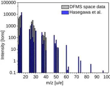
2 0 3 0 4 0 5 0 6 0 7 0 8 0 9 0 1 0 0 0 . 1 1 1 0 1 0 0 1 0 0 0 1 0 0 0 0 1 0 0 0 0 0 In te n s it y [ Io n s ] m / z [ u / e ] D F M S s p a c e d a t a H a s e g a w a e t a l .

Fig. 17. Comparison to the Hasegawa model. The plot compares the

calculated number of ions for DFMS space data with the Hasegawa et al.(1992) model A. For the DFMS, only saturated species and the remaining number of unsaturated species are taken into account, the fragmentation products of the saturated are subtracted.

the aphelion phase, from the north as well as from the south. The uppermost layers may therefore have been depleted from methane when Rosetta arrived at the comet. These layers then eroded later on and revealed fresh material. Higher aliphatic compounds are less abundant than methane by about a factor of ten. However, propane, butane, and pentane have very similar abundances. ROSINA has clearly detected aromatic hydrocar-bons, namely benzene and toluene, which are roughly on the 1% level compared to methane. Toluene has most probably also been detected by Ptolemy, one of the mass spectrometers on the lander

Philae (Altwegg et al. 2017). Aliphatic saturated hydrocarbons

are hard to detect using remote sensing because they have small

dipole moments. Table 1 fromHerbst & Van Dishoeck(2009)

gives a list of detected species in the interstellar medium that contains only unsaturated molecules. These have a much larger

dipole moment. Figure17shows resulting relative abundances

from the Hasegawa model for the ISM (Hasegawa et al. 1992).

Although the results from the model are not directly compara-ble to our list of species, which contains in addition to saturated, unsaturated, and cyclic molecules fragments from the electron impact ionization in the instrument, the relative abundances with mass between the modeled data and our measured data are quite comparable.

5. Conclusions

The study of our DFMS calibration campaign and of DFMS space data allowed us to identify and quantify pure hydrocarbons released by comet 67P. Cometary bulk material, most observ-able during May 2015, shows several pure aliphatic and aromatic hydrocarbons in addition to mixed CH-compounds such as CHO- or HCN-compounds. Hereby, an in depth analysis of the May 2015 space data revealed methane, ethane, propane, ben-zene, and toluene. Furthermore, it indicates butane and pentane in the cometary bulk because fragments of both species could be identified. However, this analysis excludes hexane, heptane, and octane in the cometary coma. This is most probably due to the large distance from the comet and the detection limit of DFMS. Investigations during different measurement periods confirm the

picture, but also suggest a contribution of the cometary dust on hydrocarbons. This is a consequence of cometary dust often being much warmer than the surface of the comet, which leads

to outgassing of lesser volatile species (seeLien 1990).

Measure-ments on 9 July 2015 and in March 2015 and on 5 September

2016 (seeAltwegg et al. 2017) are proof of the presence of

hex-ane and suggest the presence of hepthex-ane in the coma. In contrast to all other hydrocarbons, these species are only observable in a limited number of spectra, suggesting that the presence is con-nected to events with higher dust activity. Investigation over a full month shows that hydrocarbon abundances vary with time, but there is no clear correlation with latitude. This might in part be caused by dust being a distributed source for low-volatility hydrocarbons. Finally, the heliocentric distance of the comet sig-nificantly affects the abundances because hydrocarbons tend to

correlate far more strongly with CO2than with water (seeGasc

et al. 2017).

Acknowledgements. This work was supported by the following institutions and agencies: University of Bern was funded by the State of Bern, the Swiss National Science Foundation and by the European Space Agency PRODEX Program. Work at Southwest Research institute was funded by Jet Propulsion Laboratory (subcontract no. 1496541), at the University of Michigan by NASA (contract JPL–1266313), by CNES grants at Laboratoire Atmospheres, Milieux, Obser-vations Spatiales, and at Royal Belgian Institute for Space Aeronomy by the Belgian Science Policy Office via PRODEX/ROSINA PEA 90020. Furthermore, we would like to thank all the engineers, technicians and scientists involved in the mission, the Rosetta Spacecraft and the ROSINA team. Rosetta is an ESA mis-sion with contributions from its member states and NASA. Thus we acknowledge herewith the work of the whole ESA Rosetta team. All ROSINA data has been released to the public PSA archive of ESA (https://www.cosmos.esa.int/

web/psa/rosetta) and to the PDS archive of NASA.

References

Altwegg, K., Balsiger, H., Berthelier, J.-J., et al. 2017,MNRAS, 469, 130

Balsiger, H., Altwegg, K., Bochsler, P., et al. 2007,Space Sci. Rev., 128, 745

Bibring, J.-P., Taylor, M. G. G. T., Alexander, C., et al. 2015,Science, 349, 493

Bockelée-Morvan, D., Lis, D., Wink, J., et al. 2000,A&A, 353, 1101

Calmonte, U., Altwegg, K., Balsiger, H., et al. 2016,MNRAS, 462, S253

Capaccioni, F., Coradini, A., Filacchione, G., et al. 2015,Science, 347, aaa0628

Dello Russo, N., Kawakita, H., Vervack Jr R. J., & Weaver, H. A. 2016,Icarus, 278, 301

Fray, N., Bardyn, A., Cottin, H., et al. 2016,Nature, 538, 72

Gasc, S., Altwegg, K., Fiethe, B., et al. 2017,Planet. Space Sci., 135, 64

Glassmeier, K.-H., Boehnhardt, H., Koschny, D., Kührt, E., & Richter, I. 2007,

Space Sci. Rev., 128, 1

Goesmann, F., Rosenbauer, H., Bredehöft, J. H., et al. 2015, Science, 349, aab0689

Graf, S., Altwegg, K., Balsiger, H., et al. 2004,J. Geophys. Res. Planets, 109

Guilbert-Lepoutre, A., Rosenberg, E. D., Prialnik, D., & Besse, S. 2016,

MNRAS, 462, S146

Hasegawa, T. I., Herbst, E., & Leung, C. M. 1992,ApJS, 82, 167

Herbst, E., & Van Dishoeck, E. F. 2009,ARA&A, 47, 427

Laeuter, M., Kramer, T., Rubin, M., & Altwegg, K. 2019,MNRAS, 483, 852

Le Roy, L., Altwegg, K., Balsiger, H., et al. 2015,A&A, 583, A1

Lien, D. J. 1990,ApJ, 355, 680

Mattauch, J., & Herzog, R. 1934,Z. Astrophys., 89, 786

Mitchell, D., Lin, R., Anderson, K., et al. 1987,Science, 237, 626

Mumma, M. J., & Charnley, S. B. 2011,ARA&A, 49, 471

Nevejans, D., Neefs, E., Kavadias, S., Merken, P., & Van Hoof, C. 2002,Int. J. Anal. Spectrom., 215, 77

Quirico, E., Moroz, L., Schmitt, B., et al. 2016,Icarus, 272, 32

Rubin, M., Altwegg, K., Balsiger, H., et al. 2015,Science, aaa6100

Schläppi, B., Altwegg, K., Balsiger, H., et al. 2010,J. Geophys. Res. Space Phys., 115

Stein, S. E., 2018, NIST Chemistry WebBook, NIST Standard Reference Database Number 69, eds. P. J. Linstrom & W. G. Mallard (Gaithersburg: National Institute of Standards and Technology)

Taylor, M. G. G. T., Alexander, C., Altobelli, N., et al. 2015,Science, 347, 387

Vincent, J.-B., A’Hearn, M. F., Lin, Z.-Y., et al. 2016,MNRAS, 462, S184

Westermann, C. B., Luithardt, W., Kopp, E., et al. 2001,Meas. Sci. Technol., 12, 1594

Appendix A: Sensitivities

Table A.1. Sensitivities.

Compound Sensitivity Source

Octane 2.56E–20 A Heptane 2.61E–20 A Toluene 2.05E–19 A Hexane 1.22E–18 B Benzene 4.66E–18 B Pentane 6.17E–20 A Butane 5.16E–19 A Propane 2.48E–19 A Ethane 2.29E–19 A Methane 8.66E–19 A Water 2.31E–19 A

Notes. A: DFMS calibration. B: calculated based on the cross section.

Appendix B: DFMS fragmentation patterns

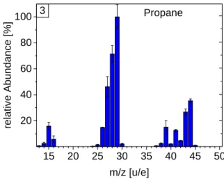
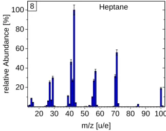
DFMS fragmentation pattern for all calibrated hydrocarbons. The patterns are given in percentage relative to the fragment with the highest abundance (relative fragmentation). Patterns are sorted by increasing mass: methane, ethane, propane, butane, pentane, hexane, toluene, heptane, and octane.

1 3 1 4 1 5 1 6 2 0 4 0 6 0 8 0 1 0 0 1 M e t h a n e re la ti v e A b u n d a n c e [ % ] m / z [ u / e ]

Fig. B.1.Fragmentation pattern of methane.

1 5 2 0 2 5 3 0 2 0 4 0 6 0 8 0 1 0 0 E t h a n e re la ti v e A b u n d a n c e [ % ] m / z [ u / e ] 2

Fig. B.2.Fragmentation pattern of ethane.

1 5 2 0 2 5 3 0 3 5 4 0 4 5 5 0 2 0 4 0 6 0 8 0 1 0 0 P r o p a n e re la ti v e A b u n d a n c e [ % ] m / z [ u / e ] 3

Fig. B.3.Fragmentation pattern of propane.

1 5 2 0 2 5 3 0 3 5 4 0 4 5 5 0 5 5 6 0 2 0 4 0 6 0 8 0 1 0 0 B u t a n e re la ti v e A b u n d a n c e [ % ] m / z [ u / e ] 4

Fig. B.4.Fragmentation pattern of butane.

2 0 3 0 4 0 5 0 6 0 7 0 2 0 4 0 6 0 8 0 1 0 0 re la ti v e A b u n d a n c e [ % ] m / z [ u / e ] 5 _{P e n t a n e}

2 0 3 0 4 0 5 0 6 0 7 0 8 0 9 0 2 0 4 0 6 0 8 0 1 0 0 H e x a n e re la ti v e A b u n d a n c e [ % ] m / z [ u / e ] 6

Fig. B.6.Fragmentation pattern of hexane.

2 0 3 0 4 0 5 0 6 0 7 0 8 0 9 0 1 0 0 2 0 4 0 6 0 8 0 1 0 0 T o l u e n e re la ti v e A b u n d a n c e [ % ] m / z [ u / e ] 7

Fig. B.7.Fragmentation pattern of toluene.

2 0 3 0 4 0 5 0 6 0 7 0 8 0 9 0 1 0 0 2 0 4 0 6 0 8 0 1 0 0 re la ti v e A b u n d a n c e [ % ] m / z [ u / e ] H e p t a n e 8

Fig. B.8.Fragmentation pattern of heptane.

2 0 3 0 4 0 5 0 6 0 7 0 8 0 9 0 1 0 0 1 1 0 2 0 4 0 6 0 8 0 1 0 0 re la ti v e A b u n d a n c e [ % ] m / z [ u / e ] O c t a n e 9