Publisher’s version / Version de l'éditeur:
Vous avez des questions? Nous pouvons vous aider. Pour communiquer directement avec un auteur, consultez la
première page de la revue dans laquelle son article a été publié afin de trouver ses coordonnées. Si vous n’arrivez pas à les repérer, communiquez avec nous à PublicationsArchive-ArchivesPublications@nrc-cnrc.gc.ca.
Questions? Contact the NRC Publications Archive team at
PublicationsArchive-ArchivesPublications@nrc-cnrc.gc.ca. If you wish to email the authors directly, please see the first page of the publication for their contact information.
https://publications-cnrc.canada.ca/fra/droits
L’accès à ce site Web et l’utilisation de son contenu sont assujettis aux conditions présentées dans le site LISEZ CES CONDITIONS ATTENTIVEMENT AVANT D’UTILISER CE SITE WEB.
Technical Report (National Research Council of Canada. Canadian Hydraulics Centre); no. CHC-TR-077, 2011-03-01
READ THESE TERMS AND CONDITIONS CAREFULLY BEFORE USING THIS WEBSITE.
https://nrc-publications.canada.ca/eng/copyright
NRC Publications Archive Record / Notice des Archives des publications du CNRC : https://nrc-publications.canada.ca/eng/view/object/?id=a2a8275f-1844-45a9-a79c-81dcdda441fa https://publications-cnrc.canada.ca/fra/voir/objet/?id=a2a8275f-1844-45a9-a79c-81dcdda441fa
Archives des publications du CNRC
For the publisher’s version, please access the DOI link below./ Pour consulter la version de l’éditeur, utilisez le lien DOI ci-dessous.
https://doi.org/10.4224/17506211
Access and use of this website and the material on it are subject to the Terms and Conditions set forth at The Effect of floe size on the flow of ice covers through converging channels
The Effect of Floe Size on the Flow of Ice Covers
through Converging Channels - DRAFT
Mohamed Sayed, Ivana Kubat and David Watson
Technical Report CHC-TR-077
The Effect of Floe Size on the Flow of Ice Covers
through Converging Channels
Mohamed Sayed, Ivana Kubat and David Watson Canadian Hydraulics Centre
National Research Council of Canada Ottawa, Ont. K1A 0R6
Canada
Technical Report CHC-TR-077
ABSTRACT
The present report describes work done to examine the effect of floe size on the drift of ice covers. Flow through a converging channel is used as a test case. The testing examined the drift of continuous ice covers as well as ice covers consisting of assemblies of distinct deformable floes. The results showed that the drift of all ice cover types through converging channels can be represented by a relationship between two non-dimensional variables. The first variable is a non-non-dimensional drift velocity (normalized by the free drift velocity). The second variable represents the ratio between the environmental driving force (e.g. wind drag) and the strength of the ice cover.
The results showed that the existence of distinct floes in the ice cover slows the drift through constrictions. The decrease of the drift velocity becomes more pronounced with increasing floe sizes. Moreover, the effects of floe size also become apparent for relatively small environmental driving forces. For higher forces (e.g. higher wind velocities), even large floes are pushed through the constrictions.
The present approach proved to be capable of quantifying the influence of floe size on the drift. The present work can thus be extended to serve as a basis for developing forecast products to guide the prediction of the drift of ice covers containing relatively large floes. Such products will require examining a wider range of geometries, floe sizes and ice properties. The report suggests that analysis of available records can be used to provide forecast plots for specific locations of interest.
TABLE OF CONTENTS
1.0 INTRODUCTION ... 9
2.0 SCOPE ... 10
3.0 CONTINUOUS ICE COVER ... 10
4.0 LARGE FLOES ... 14
5.0 SMALL FLOES ... 17
6.0 UNIFORM ICE COVER WITH TENSILE STRENGTH ... 19
7.0 NON-DIMENSIONAL FLOW RATES ... 21
8.0 CONCLUSIONS ... 23
LIST OF FIGURES
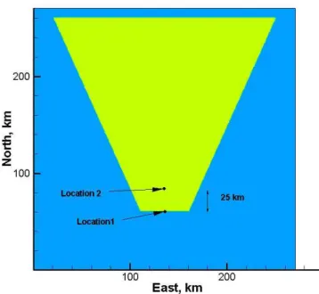
Figure 1: Sketch of the test channel. The sides are inclined 300 to the vertical. ... 11
Figure 2: Distributions of ice concentration, and pressure after 4.5 days from the start of the simulation. ... 12
Figure 3: Velocity vectors near the land boundary and exit, time= 4.5 days. ... 13
Figure 4: Velocity at the exit of the channel versus time for a continuous ice cover. ... 13
Figure 5: The initial ice cover consisting of large 20 km floes and smaller 5 km floes included within the interstices. Concentration= 0.7. ... 15
Figure 6: Distributions of ice concentration, and pressure after 10 days from the start of the simulation, case of large floes. ... 16
Figure 7: velocity vectors after 10 days, cast of large floes. ... 16
Figure 8: Velocity versus time, case of large floes. ... 17
Figure 9: The initial ice cover consisting of small 5 km floes. Concentration= 0.7. ... 18
Figure 10: Distributions of ice concentration, and pressure after 10 days from the start of the simulation, case of small floes. ... 19
Figure 11: Distributions of ice concentration, and pressure after 4.5 days from the start of the simulation, case of continuous ice cover with tensile strength Pt/Pc= 0.1. ... 20
The Effect of Floe Size on the Flow of Ice Covers
through Converging Channels
1.0 INTRODUCTION
The present work aims to develop a methodology for quantifying the effect of floe size on the drift of ice covers. Such effects are widely recognized as paramount for accurate ice forecasts, particularly at resolutions of interest to offshore operations. Still, only rules of thumb and forecasters’ experience are used to forecast the drift of ice covers which include large floes. The problem has so far been beyond forecast model because of many complexities. Continuum models face great difficulties in tracking the interfaces between floes, and accounting for the varying ice properties between the interior and edges of floes. Although discrete element methods can track the interaction between various rigid bodies, the floes undergo deformation, splitting and breaking. The present approach builds on earlier work that makes it possible to keep track of the interfaces between floes, and to introduce the appropriate ice strength for the floe and interface conditions.
Previous work on the drift of ice covers through converging channels provides a basis for examining the effects of floe size. Converging channels represent an idealization for many locations of interest to ice forecasting. Additionally, the nature of the deformation of ice covers as they drift through constrictions provides an ideal situation for examining the interaction between floes. Kubat et al. (2006) reported on the studies of flow through converging channels. That paper also includes a description of available relevant literature and the ice dynamics model, which is used in the present investigation. Another recent study by Sayed and Kubat (2010) provides the basis for the present work. The report of Sayed and Kubat (2010) examined a non-dimensional grouping of variables that appeared to provide a concise means for predicting drift through converging channels. That formulation was proposed by Flato (2010). The present study seeks to extend that formulation to account for floe sizes.
One of the significant issues in modelling the interaction between floes is accounting for ice properties. Within the interior of each floe, intact ice is expected to posses tensile strength. Alternatively, at the edges of floes, tensile strength should disappear. It is noted that yield conditions employed in large scale forecasting include only small tensile strengths. The yield condition of Savage (2008) includes tensile strength, and is used in the present work.
This report describes the work carried out during 2010/2011 as outlined in a Memorandum of Understanding (MOU) between the Canadian Ice Service (CIS) and the Canadian Hydraulics Centre (NRC-CHC). The report is intended as a documentation of the results.
2.0 SCOPE
The scope of the project was outlined in the MOU between CIS and NRC-CHC. The initial test matrix was revised during monthly reviews of the progress of work. The test matrix consisted of approximately 30 simulations. The choice of simulation conditions was aimed at examining the following cases:
1. Flow of a uniform ice cover without distinct floes: That scenario serves as a reference case for comparison with cases with pronounced floe sizes. Geometry of the channel and width of the exit (50 km) were chosen are representative of locations of interest to CIS. Test conditions were chosen to represent varied ratios between environmental forcing and ice resistance (or strength) in order to examine a wide range of drift velocities.
2. An ice cover consisting of relatively large floes of 20 km diameters: A size distribution including also smaller floes is used in order to attain the required initial packing (ice concentration).
3. An ice cover consisting of smaller ice floes of 5 km diameters.
4. A uniform ice cover with tensile ice strength equal to that used to model the interior of the floes. Note that the reference case 1 employs the common yield envelope of Hibler which accounts for only small tensile strength.
3.0 CONTINUOUS ICE COVER
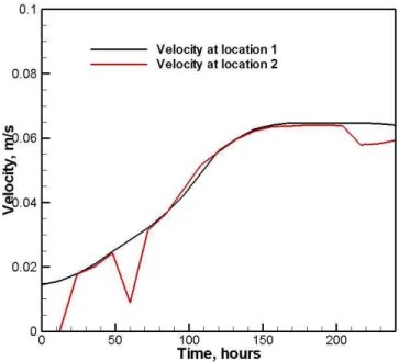
As a reference case, an ice cover of initially uniform thickness and concentration is examined. The geometry used in the simulation is shown in Figure 1. The initial thickness is 1 m, and the initial concentration is 0.7. A steady uniform Northerly wind drives the ice through the exit of the converging channel. Water current is zero, and Coriolis force is neglected. Thus the flow would be symmetrical around the centre line of the channel. Figure 1 shows two locations where drift velocity of the ice is recorded. Velocity at location 2, which 25 km above the exit is used in flow rate calculations since it is more representative of the flow rate through the constriction.
The test cases also use Hibler’s elliptical yield envelop with the following parameter values: P* = 2 x 10⁴ N/m and e=2. A rectangular grid of 0.5 km cell size is used in the calculations.
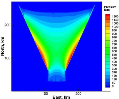
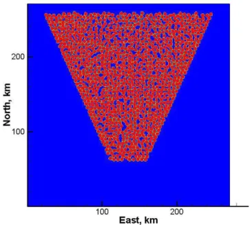
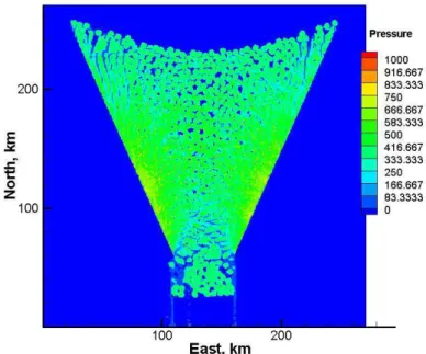
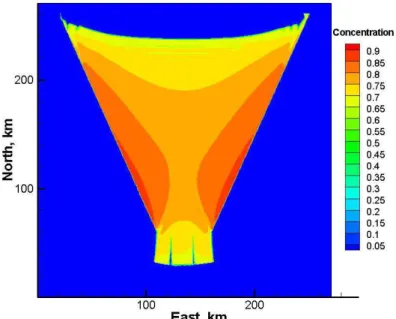
Test runs were done using a range of values for wind velocity. As an example of the output, the resulting distributions of ice concentration and pressure (mean normal stress) for a wind velocity of 3.5 m/s are shown in Figure 2. Those distributions represent conditions after 4.5 days from the start of a simulation. Thickness changes were very small to show on the plots.
Figure 1: Sketch of the test channel. The sides are inclined 30o to the vertical. The results shown in Figure 2 correspond to an initial ice thickness of 1 m, and an initial concentration of 0.7.
(b) Distribution of the pressure (mean normal stress)
Figure 2: Distributions of ice concentration, and pressure after 4.5 days from the start of the simulation.
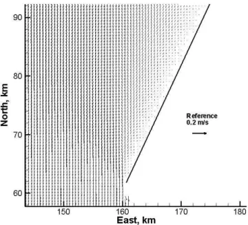
Velocities are difficult to plot over the entire channel. Figure 3 shows the velocity vectors near the land boundary and through part of the exit. The velocities apparently drop within a relatively narrow zone in the vicinity of the land boundary.
The resulting velocities at locations 1 and 2 are plotted versus time in Figure 4. As expected the velocity reaches a steady value. We note that the steady value of the velocity at location 2 is used in all subsequent calculations of the non-dimensional velocities. Other tests used wind velocities of 0.5 m/s, 1.0 m/s, and 2.0 m/s. The results follow the patterns shown above (Figure 2 to Figure 4). The resulting velocities at the exit are used to calculate non-dimensional flow rates as will be shown in the subsequent sections of this report.
Figure 3: Velocity vectors near the land boundary and exit, time = 4.5 days.
4.0 LARGE FLOES
Figure 5 shows the initial ice cover that includes large 20 km floes. Smaller 5 km floes are embedded within the interstices to bring the initial concentration to 0.7. The channel geometry and direction of wind forcing are the same as described in the previous section for the continuous ice cover. Ice thickness is 1 m.
Ice properties were introduced as follows. For the interior of the ice floes, the shifted elliptical yield envelope of Savage (2008) is used. That yield conditions allows for tensile strength which is expected for the intact ice of each floe. The tensile strength is represented by the parameter Pt, while the compressive strength is represented by Pc.
Note that the yield envelope reduces to the familiar Hibler’s ellipse when Pt = 0 and Pc =
P*. The tests were done using a tensile to compressive strength ratio Pt / Pc = 0.2. At the
edges of the floes, the tensile strength is considered to be zero. In that case the usual yield envelope of Hibler is used.
A numerical scheme was devised to identify the two types of ice: interior to floes, and at floe edges. The initial configuration included an identification number for each floe (floe id). That identification number was tracked for all the ice from the start of each simulation run (tracking was convenient because of the Particle-In-Cell advection method). During the simulations the floe id numbers within each grid cell were examined. Ice was considered to have a tensile strength if all identification numbers were equal (ice belongs to a single floe). Otherwise, if more than one identification numbers were found, the cell was considered to belong to an interface between floes, and tensile strength was set to zero. Additionally, if tensile yield was reached at any point during a simulation run, an attribute signifying fracture was introduced. That ice was considered to have no tensile strength throughout the simulation.
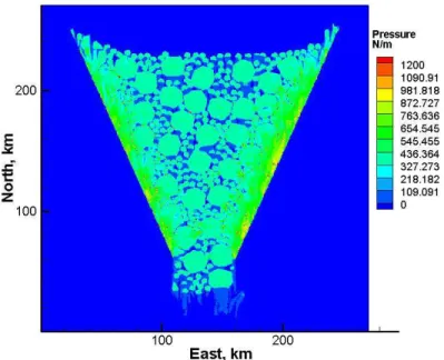
The results are illustrated in Figure 6 by showing concentration and pressure distributions for a case of wind velocity of 3.5 m/s. The plots are shown for an elapsed time value of 10 days. Ice velocities vectors near the exit are also shown in Figure 7, which shows that individual floes drift at somewhat varying velocities from each other. Figure 8 shows plots of the velocities versus time for locations 1 and 2.
Figure 5: The initial ice cover consisting of large 20 km floes and smaller 5 km floes included within the interstices. Concentration = 0.7.
(b) Distribution of the pressure (mean normal stress), case of large floes.
Figure 6: Distributions of ice concentration, and pressure after 10 days from the start of the simulation, case of large floes.
Figure 8: Velocity versus time, case of large floes.
5.0 SMALL FLOES
An ice cover consisting of smaller 5 km floes was tested. The initial configuration of the floes is shown in Figure 9. Wind velocities of 2.0 m/s, 2.5 m/s, 3.5 m/s and 5.0 m/s were used in the tests. The initial concentration is 0.7 and ice thickness is 1 m.
Examples of the resulting distributions of ice concentration and pressures are shown in Figure 10. Those results correspond to a wind velocity of 3.5 m/s, and elapsed time of 10 days. The velocities follow similar patterns to those reported above.
Figure 9: The initial ice cover consisting of small 5 km floes. Concentration = 0.7.
(b) Distribution of the pressure (mean normal stress), case of small floes.
Figure 10: Distributions of ice concentration, and pressure after 10 days from the start of the simulation, case of small floes.
6.0 UNIFORM ICE COVER WITH TENSILE STRENGTH
A uniform ice cover of initial thickness of 1 m and initial concentration of 0.7 was assumed to have a tensile strength. A tensile to compressive strength ratio of 0.1 was used. It should be noted that a range of values for that ratio was examined in preliminary tests. Numerical problems started to come-up for ratios of 0.2 and higher. We also note that a ratio of 0.1 is commensurate with values cited in literature on ice properties (Savage, 2008).
As an example of the results, Figure 11 shows distributions of ice concentration and pressure for a wind velocity of 3.5 m/s. The plots in Figure 11 are for an elapsed time of 4.5 days.
(a) Distribution of ice concentration.
(b) Distribution of the pressure (mean normal stress).
Figure 11: Distributions of ice concentration, and pressure after 4.5 days from the start of the simulation, case of continuous ice cover with tensile strength Pt/Pc= 0.1.
7.0 NON-DIMENSIONAL FLOW RATES
Following the approach used by Sayed and Kubat (2010), the results are represented in terms of two non-dimensional groups. That approach came from a suggestion by Flato (2010) to use a dimensionless number representing the ratio between the driving force and ice resistance to characterize the restriction to the flow. At one extreme, when ice strength is relatively low and land boundaries offer no constriction, the ice would move at the free drift velocity. On the other extreme, when ice is relatively strong and land boundaries restrict the flow, arching may occur and the flow would completely stop. The effect of the constriction is thus examined using two dimensionless groups.
The first dimensionless term, representing the relative velocity of the ice is
freedrift exit u
u
u′= (1)
where uexit is the velocity at the exit. We consider that exit velocity is represented by the value above the potential arch (see Fig. 1 a). The velocity at a distance 25 km above the exit is used in the present report. The free drift velocity, ufree drift, represents the value obtained when ice strength is set to zero.
The second dimensionless number, F, is given by
W h P F τ * = (2)
where P* is the familiar Hibler’s strength parameter, h is ice thickness, τ is the forcing shear stress (due to wind), and W is the width of the exit. Note that the nominator in Eq. 2 represents the resistance to flow, and the denominator represents the driving force. Thus, a small value of F corresponds to near free drift conditions. A high value for F signifies relatively large resistance to flow and a potential for arching.
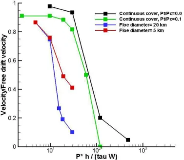
All results from the present work were transformed to the non-dimensional groups u’ and
F. The resulting plot is shown in Figure 12. Using a log-scale for the horizontal axis,
which represents the variable F, proved to give a clear view of the results.
Figure 12 summarizes the results of all the simulation runs. The decrease of u’ with increasing F follows the expected trend. The important issue for the present study is the effect of floe size. Evidently discrete floes reduce the flow rate. Moreover, the decrease in flow rate becomes more pronounced as floe size increases. It is also of note that floe size effects were relatively small for large values of environmental forcing (e.g. due to wind drag). The higher drag values would force the floes through the constrictions, with little effect from ice resistance.
The continuous ice cover with tensile strength corresponds to lower flow rates than those obtained for no tensile strength. The unexpected result is that a continuous ice cover with tensile strength yielded higher flow rates than those for discrete floes. Clarifying that observation requires further testing. A possible explanation, though, may relate to the manner in which the intact ice fractures and deforms. It may be relatively easy for large fractures to propagate through the continuous ice cover. The existence of floes may arrest (or stop) the propagation of fractures through the ice cover.
Figure 12: Plot of the relationship between the two dimensionless numbers, u’ and F.
8.0 CONCLUSIONS
The present report documents the results done during 2010/2011 on a project aimed at developing a method to quantify the influence of floe size on ice drift. The work builds on earlier investigations of ice flow through converging channels. Previous results showed that the drift of ice covers through a converging channel is governed by a non-dimensional variable that represents the ratio between the environmental forces and ice cover strength. The present work extends those investigations to examine the behaviour of ice covers consisting of relatively large distinct and deformable floes. Tests examined the following types of ice covers: continuous ice cover with no tensile strength, ice cover consisting of a mix of large 20 km floes and smaller 5 km floes, ice cover consisting of 5 km floes, and a continuous ice cover with tensile strength (representing intact competent ice).
The conclusions are summarized as follows:
• The drift of all types of ice covers follows a relationship between a dimensional drift velocity (normalized with free drift speed) and a non-dimensional number expressing the ratio between the magnitude of the environmental driving force and the strength of the ice cover.
• The existence of distinct floes in the ice cover slows the drift through constrictions. The decrease of the drift velocity becomes more pronounced with increasing floe sizes.
• The effects of floe size also become apparent for relatively small environmental driving forces. For higher forces (e.g. higher wind velocities) forces the floes through the constrictions thereby reducing the effects of floe size.
• The present approach proved to be capable of quantifying the influence of floe size on the drift. The present work can thus be extended to cover wider range of geometries and floe size distributions.
The conclusions can serve as a basis for developing forecast products to guide the prediction of the drift of ice covers containing relatively large floes. Such products will require further work to systematically cover the range of conditions which may be of interest to operational forecasters. Developments may examine a wider range of channel geometries, size distributions of floes, and ice properties (to correspond to seasonal variations of ice strength).
A suggestion for the use of the results may be as follows. Specific locations can be established (e.g. parts of Lancaster Sound or Nares Strait). Available data concerning drift and environmental forcing can then be analyzed. Drift estimates and documenting floe sizes will require analysis of available imagery. The drift estimates, floe size data, and environmental records (e.g. wind, tide) can be used to develop curves such as those shown in Figure 12 for each site of interest. Such a product will guide the forecasting of ice drift through constrictions, effect of large floes, and risk of arch formation. We note that developing such products does not require further modelling work.
9.0 REFERENCES
Flato, G. (2010). “Personal communications”.
Kubat, I, Sayed, M., Savage, S.B., and Carrieres, T. (2006). “Flow through converging channels,” International Journal of Offshore and Polar Engineering, Vol. 106, No. 4, pp. 268-273.
Kubat, I., and Sayed, M. (2010). “The flow of continuous and broken ice covers through converging channels,” Technical Report CHC-TR-073, May 2010, Canadian Hydraulics centre, National Research Council, Ottawa, Ontario, K1A 0R6.
Savage, S.B. (2008). “Elliptical yield function for modeling cohesion resulting from freeze-bonding in sea ice fields,” Report to the Canadian Hydraulics Centre, National Research Council, February 27, 2008.