HAL Id: hal-01342629
https://hal.archives-ouvertes.fr/hal-01342629
Submitted on 6 Jul 2016
HAL is a multi-disciplinary open access
archive for the deposit and dissemination of
sci-entific research documents, whether they are
pub-lished or not. The documents may come from
teaching and research institutions in France or
abroad, or from public or private research centers.
L’archive ouverte pluridisciplinaire HAL, est
destinée au dépôt et à la diffusion de documents
scientifiques de niveau recherche, publiés ou non,
émanant des établissements d’enseignement et de
recherche français ou étrangers, des laboratoires
publics ou privés.
GPR measurements to assess the Emeelt active fault’s
characteristics in a highly smooth topographic context,
Mongolia
Jean-Rémi Dujardin, Maksim Bano, Antoine Schlupp, Matthieu Ferry,
Ulziibat Munkhuu, Nyambayar Tsend-Ayush, Bayarsaikhan Enkhee
To cite this version:
Jean-Rémi Dujardin, Maksim Bano, Antoine Schlupp, Matthieu Ferry, Ulziibat Munkhuu, et al..
GPR measurements to assess the Emeelt active fault’s characteristics in a highly smooth
topo-graphic context, Mongolia. Geophysical Journal International, Oxford University Press (OUP), 2014,
�10.1093/gji/ggu130�. �hal-01342629�
Geophysical Journal International
Geophys. J. Int. (2014)198, 174–186 doi: 10.1093/gji/ggu130
Advance Access publication 2014 April 30 GJI Marine geosciences and applied geophysics
GPR measurements to assess the Emeelt active fault’s characteristics
in a highly smooth topographic context, Mongolia
Jean-R´emi Dujardin,
1Maksim Bano,
1Antoine Schlupp,
1Matthieu Ferry,
2Ulziibat Munkhuu,
3Nyambayar Tsend-Ayush
3and Bayarsaikhan Enkhee
31Institut de Physique du Globe de Strasbourg, CNRS UMR 7516, Universit´e de Strasbourg, Strasbourg, France. E-mail:[email protected] 2University of Montpellier 2, G´eosciences, Montpellier, France
3Research Center of Astronomy and Geophysics, Mongolian Academy of Sciences, Ulaanbaatar, Mongolia
Accepted 2014 April 2. Received 2014 April 2; in original form 2013 August 9
S U M M A R Y
To estimate the seismic hazard, the geometry (dip, length and orientation) and the dynamics (type of displacements and amplitude) of the faults in the area of interest need to be understood. In this paper, in addition to geomorphologic observations, we present the results of two ground penetrating radar (GPR) campaigns conducted in 2010 and 2011 along the Emeelt fault in the vicinity of Ulaanbaatar, capital of Mongolia, located in an intracontinental region with low deformation rate that induces long recurrence time between large earthquakes. As the geomorphology induced by the fault activity has been highly smoothed by erosion processes since the last event, the fault location and geometry is difficult to determine precisely. However, by using GPR first, a non-destructive and fast investigation, the fault and the sedimentary deposits near the surface can be characterized and the results can be used for the choice of trench location. GPR was performed with a 50 MHz antenna over 2-D lines and with a 500 MHz antenna for pseudo-3-D surveys. The 500 MHz GPR profiles show a good consistency with the trench observations, dug next to the pseudo-3-D surveys. The 3-D 500 MHz GPR imaging of a palaeochannel crossed by the fault allowed us to estimate its lateral displacement to be about 2 m. This is consistent with a right lateral strike-slip displacement induced by an earthquake around magnitude 7 or several around magnitude 6. The 2-D 50 MHz profiles, recorded perpendicular to the fault, show a strong reflection dipping to the NE, which corresponds to the fault plane. Those profiles provided complementary information on the fault such as its location at shallow depth, its dip angle (from 23◦to 35◦) and define its lateral extension.
Key words: Geomorphology; Palaeoseismology; Fractures and faults; Asia.
1 I N T R O D U C T I O N
Central Asia is known for its high level of seismic hazards, espe-cially Mongolia, which has been one of the most seismically active intracontinental regions in the world with four large earthquakes (magnitude around 8) along its active faults in the western part of the country during the last century (Khilko et al.1985). The de-formation in Mongolia is located between compressive structures related to the collision and penetration of the Indian plate into the Eurasian plate and extensive structures in the north of the country related with the Baykal rift (Tapponnier & Molnar1979; Baljinnyam
et al.1993; Schlupp1996; Bayasgalan & Jackson1999).
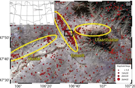
The seismic activity observed in the vicinity of Ulaanbaatar (UB), capital of Mongolia, is relatively low compared to the activity ob-served in western Mongolia. Nevertheless, since 2005, the seismic activity around UB not only has increased, but is also organized (see Fig.1) at the west of UB along two perpendicular directions, which
determine two active faults: Emeelt fault, discovered in 2008 (NNW-SSE direction, 25-km-long minimum and situated about 10 km W of UB) and Hustai fault (WSW–ENE direction, 80 km long, with its NE tip at less than 20 km west of UB); their length and mor-phology indicate that they can produce earthquakes of magnitude 6.5–7.5 (Schlupp et al.2012). Most of the Mongolian population (1.2 million over 3 million) is concentrated at UB, which is the main political and economical centre of the country. Hence, the study of seismic hazard and the estimation of the probability of future destructive earthquakes are of primary importance for the country (Dugarmaa et al.2006). Since the last large earthquake, the faults geomorphology has been highly smoothed by erosional processes and the exact location of the fault plane surface rupture is thus hidden within a several metre wide strip.
The GPR method has been proven to give good and useful re-sults to characterize faults by identifying offsets of radar reflections (Malik et al.2007; Christie et al.2009; Yalc¸iner et al.2013) and
GPR measurements to assess the Emeelt active fault’s characteristics 175
Figure 1. (a) Map of Mongolia with location of the capital, Ulaanbaatar. (b) Zoom over the area of Ulaanbaatar. Yellow lines surround the two main active faults (Emeelt and Husta¨ı) and Ulaanbaatar urban area. Red dots represent the seismicity since 2005 (after NDC data, RCAG). Note the strong alignment of the seismicity defining the Emeelt fault.
buried fluvial channel deposits (Ferry et al.2004). Many studies have shown that pseudo-3-D and 3-D GPR allow a better and reli-able interpretation than 2-D GPR profiles (e.g. Gross et al.2000,
2002,2003,2004; Tronicke et al.2004; McClymont et al.2008b). Beauprˆetre et al. (2012) used a pseudo-3-D survey in order to image a buried channel network, which allows the reconstruction of the past slip history. McClymont et al. (2008a) have used geometric attributes of 3-D GPR data to improve the visualization of active faults. Dentith et al. (2010) compared GPR data with trench results in order to study palaeofault scarps in the case of deeply weathered terrains. The concept of radar facies developed and mainly used in sedimentology (Neal2004; Pellicer & Gibson2011) is now widely considered in active tectonic context (e.g. McClymont et al.2008a,
2010).
Nevertheless, none of these studies were performed on active fault zones showing low slip rate. It is the first time that we use GPR to explore and reveal the buried traces of an active fault in such a context. Our study is focused on the Emeelt fault (Fig.1), which is associated to an intracontinental context, with moderate deforma-tion very likely much less than 1 mm yr−1(Calais et al.2003,2006; Vergnolle et al. 2007). After some preliminary geomorphologic observations and a trench dug in 2009, two GPR campaigns were conducted in 2010 and 2011. Pseudo-3-D profiles were recorded with a 500 MHz antenna over an alluvial fan and a palaeochan-nel crossed by the fault, to look for the displacement and/or the deformation of reflections and horizons. In addition, several long 50 MHz 2-D lines (about 200 m long) were realized perpendicular to the fault in a much wider area. The objective of these profiles was to look for the geometry and lateral extension of the fault at greater depth and to verify the presence of other branches.
2 C O N T E X T A N D P U R P O S E
The geomorphologic features shown by the picture in Fig.3are clearly visible on the satellite view (Fig.2). The scarp generated by the fault is clearly seen. The trace left by the fault on the surface (black arrows, Fig.2) is a couple of metre wide. It has a N143◦ direction and can be followed about 10 km on the satellite image (Fig.2, from Google Earth). If we include the seismic activity, we
can consider its length to be 25 km minimum. From the picture (Fig.3), we observe a valley in the centre that is surrounded by two hills on both sides. The scarps separate those hills and the valley. This specific geometry recalls a collapsed basin such as a normal graben system (in an extensional tectonic context) or a reverse graben (in a compressional tectonic context) or even in a transtensional context. However, due to the low slip rate (less than 1 mm yr−1) and the long recurrence time, the fault scarp has been heavily smoothed by erosional processes, hiding the precise location of the fault on the surface. In addition, no clues on the direction of the fault dip are yet observed. However, recent deposits recognized in the area allow possible dating in palaeoseismology. Thus, a first trench (referred to as trench T1) was dug in 2009 on the edge of an actual alluvial fan (Fig.2c). GPR surveys were performed only in 2010 near the trench to, on the one hand, compare both data sets and connect GPR facies with geological units and, on the other hand, identify the fault rupture at depth. Furthermore, we investigated a palaeochannel, by combining the trenches and GPR results, to estimate the cumulative displacement along the fault. A second trace, parallel to the first one, is observed on a smaller area (white arrows, Figs2and3). Both traces show a similar signature on the surface, and raise the question of a possible second branch.
3 D AT A A C Q U I S I T I O N A N D P R O C E S S I N G
3.1 Methodology of GPR acquisition
Ground penetrating radar (GPR) is a geophysical method based on the propagation, reflection and scattering of high-frequency (from 10 MHz to 2 GHz) electromagnetic (EM) waves in the Earth (Daniels et al.1988; Jol2009). For non-magnetic rocks, it allows imaging of the electric and dielectric contrasts of the shallow sub-surface. The depth of investigation depends on the EM attenuation of the medium and the frequency used. The lower the frequency, the greater the penetration depth, which varies from a few centimetres in conductive materials up to 50 m for low conductivity (less than 1 mS m−1) media (Davis & Annan1989; Jol2009). The vertical resolution depends on the velocity of EM waves and the frequency
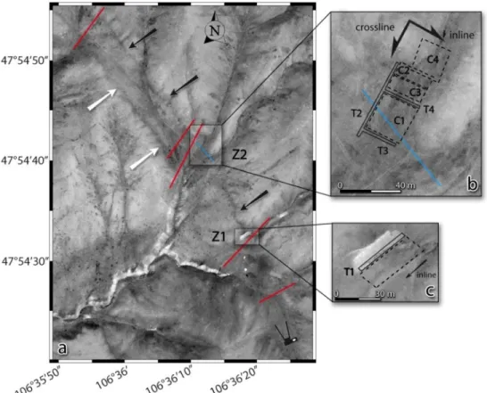
Figure 2. Aerial view of the studied area (satellite image digital globe, Google Earth 2009). Red lines indicate the location of the 50 MHz profiles (RTA). Black arrows highlight the fault trace and white arrows highlight a morphological scarp at the opposite side of the basin. Camera pictogram indicates the viewpoint of the Fig.3. (b) and (c) Zoom of areas Z1 and Z2. Trench locations are in black and the border of pseudo-3-D 500 MHz GPR cubes are with black dashed lines. The C1 and C2 cubes were recorded in 2010, while the C3 and C4 cubes were recorded in 2011 (see the text for more details). The blue line in Z2 area represents the 500 MHz profile shown in Fig.6.
Figure 3. Picture of the survey area (see Fig.2for location). Black arrows highlight the Emeelt fault scarp and white arrows show another morphological scarp. The trenches are visible on the right side.
of the antennae used. Following the λ/4 criterion (Widess1973; Jol1995; Zeng2009), it varies from 70 to 5 cm for frequencies of 50–500 MHz and velocities of 0.1–0.14 m ns−1. In general, features such as sedimentary structures, lithological boundaries, fractures and/or faults are clearly visible with GPR (Gross et al.2004; Neal
2004; Deparis et al.2007; McClymont et al.2010), even when these features differ only by small changes in the nature, size, shape, ori-entation and packing of grains (Guillemoteau et al.2012).
After the geomorphologic recognition of the Emeelt fault and a preliminary trench (T1) realized in 2009 (Fig.2), we decided to use GPR measurements to investigate subsurface deposits potentially affected by the fault on a wider area. The GPR observations should help us to decide location of future trenches. Our first objective was
to study an alluvial fan situated close to the trench T1 (referred to as Z1 area) for three reasons. First, the sedimentary deposits provide a stratigraphy that, if offset by the fault, can give us information on the geometry and dynamic of the fault, such as the dip, amplitude and direction of displacement with a non-destructive method. Secondly, sediments are usually favourable to EM propagation and thirdly, the proximity of the trench will allow us to perform a direct compar-ison of both data sets (geology and GPR). In this survey, we used a 500 MHz antenna to get detailed features at shallow depth and to have a depth of penetration and a wavelength consistent with the trench observations. We recorded 25 profiles of 40 m long on both sides of the trench T1 and parallel to it with the aim to cut through the fault. The space between profiles was 1 m and the recoding step
GPR measurements to assess the Emeelt active fault’s characteristics 177
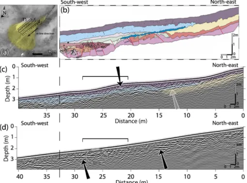
Figure 4. (a) Same as Fig.2(c)with the location of the GPR profiles (c and d) and the alluvial fan in yellow. (b) Log of the southern wall of trench T1 situated in Z1 area and dug in 2009. (c) and (d) 500 MHz GPR profiles. The profiles and the log are equally scaled; the vertical exaggeration is 1.9. Red lines in the log represent ruptures dipping mostly to the north–east from 20◦to subvertical. The three first units, purple, blue and yellow in (b) are superimposed on the profile (c) for comparison. Black arrows show horizontal reflections and grey arrow shows dipping reflection (contact between blue and yellow units). Horizontal black brackets show the position of the fault scarp at the surface.
was 0.03 m. Only 15 profiles situated south of the trench show inter-esting results and two of them are presented and discussed later on (Fig.4).
About 300 m north of Z1 area, the morphology shows two small streams crossing the fault and evidence of recent sedimentary de-posits (Fig.2). To check for the presence of hidden palaeochannels filled by sediments and cut by the fault, we recorded 11 profiles across and perpendicular to both streams using the 500 MHz an-tenna. The profiles were 80 m long with a recording step of 0.03 m. The profiles show a clear palaeochannel under the northernmost stream, well imaged by GPR (blue line in Figs 2b and 6). Con-sequently, we decided to perform the pseudo-3-D GPR survey in this area crossed by the fault (Z2 area). We opened simultaneously, due to field constraints, three trenches (T2, T3 and T4) in Z2 area; one across the fault (T2) and two parallel to it (T3 and T4). Their location and geometry are shown in Fig.2(b). The GPR survey was separated in four distinct pseudocubes, denoted 1–4. Cubes C1 and C2 were recorded in 2010, while complementary cubes C3 and C4 were recorded in 2011. An overlap of five profiles was performed between the cubes C2 and C3 in order to assess the reliability of GPR data recorded at two different periods (2010 and 2011). The main objective of this survey was to image the palaeochannel in 3-D in order to characterize any horizontal/vertical displacement caused by the fault. The pseudo-3-D approach has become a
com-mon procedure and has successfully been used in the case of active fault studies (e.g. Malik et al.2007; Beauprˆetre et al.2012). A full 3-D acquisition schema requires an interval of a quarter wavelength grid spacing (Grasmueck et al.2005) in both inline and cross-line directions of the 3-D cube. This would require one profile every 5 cm (for a mean velocity of 0.1 m ns−1) with a 500 MHz antenna. The number of profiles would then be multiplied by five compared to our current survey. As a result, and due to time constraints on the field, we have chosen the pseudo-3-D approach rather than a full 3-D schema.
The profiles were parallel to the fault direction and spaced each 25 cm (see Table1for more details about the acquisition geometry). In addition, long 2-D lines were recorded with a 50 MHz rough ter-rain antenna (RTA). The acquisition geometry is shown in Table2. The purpose of those lines was to provide additional information such as the geometry and behaviour of the fault at greater depth, the lateral extension of the fault and to test the hypothesis of a second branch in the area of investigation, which could take place along the second scarp.
The topography of all GPR profiles was recorded using differ-ential GPS. The GPS antenna was mounted on a backpack carried by an operator who was following GPR paths. The recording step of the GPS was set to twenty centimetres. Saw-tooth effects were observed on the topographic profiles due to the small movements
Table 1. Details of the pseudo-3-D surveys.
C1 (2010) C2 (2010) C2 (2011) C3 (2011) Size (inline× cross-line) 25 m× 26.5 m 24 m× 10 m 24 m× 9.5 m 20 m× 22 m
Number of inlines 107 41 38 45
Space between inlines 25 cm 25 cm 25 cm 50 cm
Number of cross-lines 26 25 9
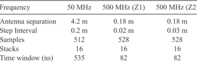
Table 2. Details of the acquisition parameters. Frequency 50 MHz 500 MHz (Z1) 500 MHz (Z2) Antenna separation 4.2 m 0.18 m 0.18 m Step Interval 0.2 m 0.02 m 0.03 m Samples 512 528 528 Stacks 16 16 16 Time window (ns) 535 82 82
of the operator while he was walking. In order to get rid of these undesirable effects, a high degree polynomial curve fitting for the data was used, instead of using raw topographic profiles.
3.2 Methodology of GPR processing
The processing of all GPR profiles has been performed with in-house software (Girard2002) written in Matlab. We used a common flow procedure involving a constant shift to adjust the time zero; a dc filter to remove the low frequencies; a flat reflections filter to remove some clutter noise (ringing caused by multiple reflec-tions between shielded antennae and the ground surface); a time varying gain function and finally a bandpass filter (elliptic-tapered filter). The time varying gain function is a smoothed version of the trace envelope calculated by Hilbert transform. Bandpass filters are of 20–150 and 100–800 MHz for the 50 and 500 MHz antennae, respectively. A velocity analysis, which is not presented here, has been done over the surveying area by analyzing diffraction hyper-bolae present in the GPR data. It gives a mean velocity of 0.135 and 0.095 m ns−1for the data collected in 2010 and 2011, respectively. These values are constant and consistent for both frequencies (500 and 50 MHz antennae). The difference in velocity is explained by the unusual humid period during the survey in 2011 compared to the 2010 dry summer. Afterwards, a Kirchhoff migration, which accounts for the topography (Lehmann & Green 2000; Heincke
et al.2005; Dujardin & Bano2013), has been applied before load-ing the data into seismic interpretation software (OpendTect). The topographic migration of each profile has been performed with a constant velocity.
4 G P R I M A G I N G R E S U L T S A N D I N T E R P R E T AT I O N
4.1 500 MHz antenna, Z1 area, description of the profiles
The filtered radar sections were visually analysed for data interpre-tation, and two of them are presented in Fig.4. They are equally scaled and are presented with a vertical exaggeration of 1.9. Their locations are shown in Fig. 4(a). The investigated alluvial fan is highlighted in yellow in Fig.4(a). The beginning of the profiles is on the NE to be in agreement with the map. The x-axis is also from NE to SW to stay consistent with the recording path of the GPR. For the interpretation, we used a combination of reflections picking with radar facies recognition. Four facies, used in the inter-pretation, are presented in Fig.5. Despite the very low penetration depth of the profiles (up to 1.5 m), special features are observed and are related to the local geology. They give us information that helps to understand the fault behaviour. The first facies is visible on both the profiles, it is either horizontal (pointed by black arrows) or with a slight dip in the direction of the topographic slope (grey arrow). Horizontal ones are related to the inner stratigraphy of the alluvial fan and were slowly deposited probably during rainfall or snow thaw. The dipping one is only observed in the first profile and
Figure 5. Facies used in the interpretation of the 500 MHz data. (a) Fa-cies having subhorizontal to slightly dipping reflections with a clear lateral continuity. (b) Subhorizontal to slightly dipping reflections with a moder-ate lmoder-ateral continuity. (c) Chaotic background with no lmoder-ateral continuity. (d) Strongly attenuated signal.
is aligned with the uphill topography. This reflection is interpreted as palaeotopography before being wrapped up by the recent allu-vial fan. Looking at the location of the profiles (Figs2and4a), we note that profile (c) is on the edge of the fan, whereas profile (d) is much more on its central part. The sediment cover, undoubtedly greater in the central part of the alluvial fan (combined with the low penetration depth), results in the disappearance in the GPR profiles of the dipping reflection, which are either deeper or eroded. The third facies, the discontinuous-chaotic background, is observed on profile (d) at the beginning and the end. It also appears in-between the horizontal reflections (profile (c): from 23 m to the end; profile (d): from 20 to 25 m). On profile (d), a special feature has to be noted: at the meeting point of facies 1 and 3, horizontal reflections are bent upward (circle in Fig.4d). This curvature can be due to the warping of the reflectors during the last fault rupture.
4.2 Comparison with the trench
Trench T1 was dug in 2009 on the edge of an actual alluvial fan (Fig.2c), just before the GPR survey. It is around 2 m deep and displays mainly typical alteration from dry and cold climate. In the first metre, we find clay and silty material, which can be responsible for the low depth of penetration the GPR signal. On the south wall of the trench, a network of synthetic and antithetic ruptures and displacing deposits has been mapped (see red lines). The dip of these ruptures ranges from 20◦ to subvertical and most of them are dipping toward the north–east. The upper units of the trench (purple, blue and yellow) have been reported on profile (c) to allow comparison. Although the profile is 5.5 m away from the trench, interfaces between units are relatable to particular reflections in the GPR profile. The dipping reflection (grey arrow) is then well aligned with the top of the yellow unit and on the left is following the bottom of the light blue one. The interface between the purple and the blue units is rather flat and fits the observed horizontal reflections (from 16 to 13 m). This is relatable to both reflections indicated by black arrows on profile (d) of Fig.4. The chaotic background in the middle of the profiles (24–29 m on profile (c) and 20–25 m on profile (d)) corresponds to the location where the purple–blue interface is dipping. However, due to the low penetration of the 500 MHz antenna, it is not possible to link the deeper units and ruptures with the GPR data.
To sum up, two different types of reflections were observed (the dipping one and the horizontal ones), and a chaotic facies is breaking off their continuity. The dipping reflection observed on the first profile is related with a previous palaeosurface, wrapped up by the alluvial fan sediments. The horizontal reflections, overlapping the dipping one on the right, are related to the inner sedimentation of the fan. However, in the middle, a chaotic facies is observed and
GPR measurements to assess the Emeelt active fault’s characteristics 179
Figure 6. Example of a 500 MHz profile crossing palaeochannels and recorded in 2010 to verify the presence of the palaeochannel in the GPR data before the precise work on ‘cubes’. Its location is displayed in Fig.2(blue line). Black arrows highlight dipping reflections (with facies, Fig.5a), which are related to the flanks of the channels.
interpreted in terms of crushed or disorganized material destroying the continuity of the layers. The location of it, in the fault zone (black brackets, Figs4c and d), is considered to be the result of the movement of the fault underneath. The horizontal reflections are bent where they meet the chaotic facies. As the fault seems to have an important strike-slip component, we cannot use these observations as a measure of displacement but only as a deformation zone.
4.3 500 MHz antenna, Z2 area, pseudo-3-D cubes
4.3.1 Description of the profiles
On the north of the Z1 area, we recorded 11 profiles of 80 m long across the two streams to verify the presence of the palaeochannel
in the GPR data and to help choose a location for the precise 3-D work. One of these profiles is presented in Fig.6. The dipping reflections showing moderate continuity are indicated by black ar-rows. The middle and the right ones clearly define the flanks of a palaeochannel. Subhorizontal reflections with moderate continuity and many diffraction hyperbolas lie in-between and are related to the sedimentary filling of the channel and the presence of many rocks. On the left side, another dipping reflection is observed. It is related to the edge of a second palaeochannel crossed by the pro-file. From those results, we decided to investigate the first channel in depth with the pseudo-3-D surveys (Dujardin et al.2012). The acquisition geometry is presented in Table2.
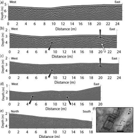
A selection of five profiles, extracted from the pseudo-3-D cubes, equally scaled and with a vertical exaggeration of 1.4 is displayed in Fig.7. The depth axes of the profiles are related to the most
Figure 7. Selection of 500 MHz profiles from the pseudo-3-D cubes in Z2 area (profiles (a)–(e) in Fig.7f), respectively. They are equally scaled and the vertical exaggeration is 1.4. Although the depth of penetration is low (from 1 to 1.5 m), many reflections, organized in two groups, are observed. The dipping reflections are related to the flanks of the channel (black arrows), while the horizontal reflections, confined between the flanks, are related to the sedimentary filling of the channel. Note on profile (b) a second deeper flank (grey arrow) probably due to interlocked channels. Profiles (b) and (c) are the same (b was recorded in 2010 and c in 2011), and display very consistent image. Note the much smaller wavelength in (c) due to the lower velocity in 2011 (soil more humid). Profile (e) is a cross-line showing only subhorizontal reflections dipping slightly downstream, which are related to the sedimentary filling.
elevated point for the four GPR cubes; thus, the zero does not ap-pear in the presented profiles. As observed in the map (Fig.7f), profiles (a)–(d) are inline profiles (from downstream to upstream). Profile (e) is a cross-line profile. Profiles (a) and (b) were recorded in 2010, and profiles (c), (d) and (e) in 2011. GPR sections (c) and (b) are both presenting the same profile, but recorded at different periods (2010 and 2011, respectively). They allow a comparison between the 2010 and the 2011 surveys. The location of the ac-tual stream is at the lowest point of the topography in the profiles (between 6 and 10 m in profiles (a)–(c)). Once again, for the inter-pretation, we use the combination of reflection picking with facies recognition as presented in Fig.5. The first facies (having subhor-izontal to slightly dipping reflections) show strong continuity and are observed in the central part of each profile. Their edges are highlighted by dipping reflections (black arrows) towards the centre of the profiles except for profile (a). The dipping reflections are the signature of the flanks of the channel. On profile (b), a second, deeper reflection is observed (grey arrow). This feature is proba-bly due to interlocked channels. Horizontal reflections are related to the sedimentation within the channel. Facies having subhorizon-tal reflections with moderate continuity and facies showing chaotic background with no lateral continuity are interlocked in between (profile (a): 14–18 m; profile (b): 11–14 m; profile (c): 13–15 m) and on the extremities of the profiles (profile (a): before 9 m and after 21 m; profile (b): before 8 m; profile (c): before 7 m). On pro-file (d), the extremities are characterized by a strong attenuation of the GPR signal corresponding to the bedrock in which the channel has been incised and filled. EM waves are then attenuated by a dif-ferent lithology. The last profile (e) presents a cross-line from north to south; it shows many continuous reflections subparallel to the topography and consistent with the first facies. They are the GPR response of the sedimentary deposition in the direction of the flow. Cross-line profiles are of great importance in the later interpretation as they allow a strong connection with inline profiles.
4.3.2 Comparison of the 2010 and 2011 data
The 2010 and 2011 profiles were then compared to check for their consistency. In 2011, the weather was very wet with heavy rainfall. This translated into a soil much more humid and a decrease in the EM wave velocity from 0.135 m ns−1in 2010 to 0.095 m ns−1 in
2011. Profile (c) is the repetition of profile (b) (Fig.7). The most striking feature is the difference in the wavelength, a direct conse-quence of the change in the velocity. The first facies is recognized in both profiles. In profile (b), it is restricted between 14 and 20 m, with the chaotic facies lying from 9 to 14 m. In profile (c), the first facies is observed in the whole channel and the dipping reflection on the left, related to the flank of the channel, is better resolved until the surface. On the right, the deeper flank is not observed on profile (c). The electrical conductivity of the ground is higher due to the increased water content and the depth of penetration has decreased, masking the deeper flank on the 2011 data. It is not possible to connect specific reflection in both profiles, but the location of the facies is in good agreement and the channel flanks are very similar in both the profiles.
4.3.3 Comparison between profiles and trenches
Fig.8(a) presents a photomosaic from the north wall of trench T4. White wires in vertical and horizontal directions highlight the 1 m spacing gridding of the trench. The profile shown in Fig.8(b) is the northern most profile of the cube C1 and is 2.5 m away from the trench T4 wall. The photomosaic and the GPR profile have the same scale, and there is no vertical exaggeration. Three main units were identified in the trench and highlighted here by brown, yellow and orange colours. The brown unit is a homogeneous silty– sandy material with some gravel scattered inside it. In some areas, gravels are gathered in thin horizontal layers, highlighted by red lines. It corresponds to the filling of the channel. The two next units are characterized by yellowish coarser material. The first one (the yellow unit) is a layer of around 50 cm thick with centimetric stones. The last unit (orange one) is very similar to the yellow unit, but with many scattered centimetric stones. The consistency between the GPR profile and the photomosaic becomes evident when we superimposed the interpretation of the trench on the profile. Bound-aries of the units match reflections observed in the GPR profiles. The gravel lens (red lines) is almost perfectly aligned with a reflec-tion in the GPR profile. The left flank of the channel (limit between the yellow and the orange unit) is as well matching a reflection and the yellow unit corresponds to an attenuated signal. On the east side, the units interfaces seem to match with dipping reflec-tions but with a lateral offset that can be explained by the distance
Figure 8. (a) Photomosaic of the north wall of T4 trench and (b) northernmost profile of cube C1, 2.5 m away from the trench wall (see location at Fig.2). Three main different units were identified in the trench highlighted here by brown, yellow and orange colours. They are superimposed on the trench and the profile for comparison. The brown is a thin brownish unit filling the channel, the yellow is a yellowish coarse deposits unit (centimetric sized) and the orange is a yellowish unit with fine material. Within the brown unit, a gravel lens is observed and highlighted by the red lines. A good consistency is observed between the GPR data and the trench. The gravel lens (red lines) is almost perfectly aligned with a reflection in the GPR profile. The left flank of the channel (limit between the yellow and the orange unit) is as well matching a reflection and the yellow unit corresponds to an attenuated signal. On the east side, the units interfaces seem to match with dipping reflections but with a lateral offset that can be explained by the distance between the trench and the GPR profile (2.5 m).
GPR measurements to assess the Emeelt active fault’s characteristics 181
Figure 9. Four GPR profiles with the palaeochannel picked in green. The 3-D surface (in colours) of the palaeochannel was deduced from the picking on all the profiles of the cube C2, C3 and C4. The red arrow shows the palaeoflow direction.
between the trench and the GPR profile (2.5 m). It is worthwhile to do the comparison for two reasons: first, it confirms our interpre-tation and secondly, it allows the connection of GPR facies with a specific lithology. Thus, first and second facies (Fig.5) are linked to the brownish, massive unit of silty sands where gravel-sized lenses are found sporadically. Third facies is linked to a coarser-grained material (centimetric size stones) showing no evidence of layering.
4.3.4 Picking of the palaeochannel
After processing, all the profiles were merged in one single survey and loaded into seismic interpretation software (Opendtect) which allows 3-D representations, depth slices and horizon picking. We tried depth slices representation and attribute analysis to improve the quality of the interpretation, but the results were disappointing due to the space between the profiles. Horizon picking was much more time-consuming but gave much more interesting results. Ow-ing to the strong disparity of the reflections, which did not allow a semi-automatic picking, we picked the channel’s flanks manually. During this step, cross-line profiles were of great importance as they permit a strong correlation of the reflections from one profile to the next one. The result of the manual picking is the 3-D surface presented in Fig.9in relation with GPR profiles (three inlines and one cross-line). The depth (from the most elevated point in the to-pography) is presented by colour scale. Green lines on the profiles represent the picking, thus the intersection between the surface and the profiles. The red arrow indicates the flow direction. The dis-played surface is obtained by interpolating the picked profiles taken from cubes C2, C3 and C4. Afterwards, the main slope of the
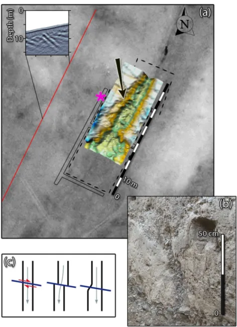
chan-nel was subtracted to provide a better interpretability of the data. The removal of the main slope straightens the channel, and the geometry of the flanks is greatly enhanced. The result is superimposed on the aerial view (Fig.13). The channel appears very heterogeneous and many bumps are observed at its bottom. The penetration depth, from 1.5 to 2 m, is often lower than the depth of the channel. Thus, the bumps are related either to a mispicking of the base of the channel or to the collapse of a flank during storm weather. The SE flank is fairly straight on its upper part and starts enlarging at around 27 m distance from the south–east corner of cube C1 (scale on Fig.13a). This enlargement is linked to the arrival in the sedimentary basin. The NW flank is as well fairly straight in its deepest part except for the shift at around 49 m distance with right lateral amplitude of about 2 m (black arrow, Fig.13).
4.4 RTA (50 MHz antenna)
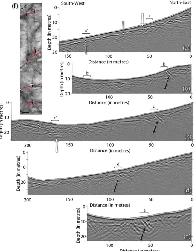
RTA profiles (50 MHz) were interpreted in a similar way as the 500 MHz profiles. They were visually analysed and interpreted us-ing a combination of GPR facies with reflection pickus-ing. The four facies used in the interpretation are shown in Fig.10. They represent reflections parallel to the topography with strong and moderate con-tinuity, facies with chaotic reflections, and finally, facies strongly attenuated. All the RTA profiles presented in Fig.11were equally scaled with a vertical exaggeration of 1.8. The x-axis is from right to left to match the direction of the profiles on the map (Figs2
and11f). Black lines on the map are the intersection of the fault scarps with the profiles. Their locations are reported on the profiles
Figure 10. Four facies (extracted from the GPR images) used in the interpretation of the 50 MHz GPR profiles. (a) Reflections showing clear lateral continuity; (b) reflections showing moderate lateral continuity; (c) chaotic background and (d) strongly attenuated signals.
Figure 11. 50 MHz GPR profiles (RTA). All the profiles are equally scaled with a vertical exaggeration of 1.8. Location of profiles (from top to bottom) is shown by red lines on the map (Fig.11f). Letters (a)–(e) show the place where morphological scarps are observed on the surface. Black arrows show the reflections from the fault plane and the change in the GPR facies that highlight the location and geometry of the fault (see the text for more details).
with the brackets. Despite the low penetration depth (10 m in the best case), much information is recovered from those profiles. First, a strong north–east dipping reflection was observed in almost every profile (indicated by black arrows). This feature is interpreted as a direct reflection from the fault plane, it gives access to the dipping direction (north–east), its dip and the exact location of the fault
(from near the surface up to 10 m depth). The dip ranges from 27◦ in the north (profiles b and c), to 23◦(profile d) increasing up to 35◦ in the south (profile e). Those reflections are exactly located under the brackets, which mean that the rupture reaches the surface. On profile (a), the reflection is not observed. However, a strong separation (white arrow) between the chaotic facies (at NE) and
GPR measurements to assess the Emeelt active fault’s characteristics 183
Figure 12. Synthesis figure of area Z1. (a) Map, displaying the RTA profiles (red lines) with the location of the fault at surface (black lines perpendicular to the profiles). Trench T1 and the 500 MHz profile are drawn in black. (b) Trench T1, (c) 500 MHz profile from Z1 (Fig.4c) and (d) RTA profile (Fig.11d). They are all equally scaled and the vertical exaggeration is 1.9. Black brackets at the top of the profiles show the location of the scarp as observed on the field and satellite image. The dashed line, surrounded by yellow zone, highlights the fault as observed in the RTA profile. It is reported as well on the 500 MHz profile and corresponds to a chaotic facies between clear horizontal reflections.
the reflection with clear continuity (at SW) is observed at the base of the scarp. Discontinuities in the reflections (pointed by grey ar-rows) are the results of the collapse of diffraction hyperbolae after migration. Reflections, showing a clear continuity, are also present in other profiles, especially in their central part (in the valley) and in profiles (c) and (d), in their upper part as well. Around the fault reflections, a chaotic facies is always observed on a width of around 30–40 m.
On the other side of the valley, neither reflections nor a change in facies are observed on profiles (a) and (b) where they cross the sec-ond scarps. However, profile (c) displays an abrupt variation as well with a change in the penetration depth (white arrow). Reflections with lateral continuity on the right are contrasting with a chaotic background on the left. This sharp contact is in good agreement with the location of the geomorphologic scarp but is not enough to conclude on its origin.
Figure 13. (a) Interpretation map of Z2 area. The interpolated 3-D surface of the channel (after subtraction of its main slope) is superimposed on the satellite image. An offset of 2 m horizontally is observed on the NW flank of the channel (see black arrow), which is consistent with a right lateral strike-slip. The pink asterisk shows the location of picture (b) in the trench where an evidence of the fault is observed. The closest RTA profile (upper left corner) shows the record and the location of the fault plane in depth. (c) Illustration of the evolution of the channel flanks due to the right lateral strike-slip. The down left flank is preserved while the down right flank is eroded after the shift. The filling of the palaeochannel fossilizes the palaeomorphology.
5 D I S C U S S I O N
In addition to geomorphology and trench observations, the GPR images obtained by using 500 and 50 MHz antennae give us impor-tant information about the Emeelt fault, which was discovered in 2008 (Schlupp et al.2012).
The GPR profiles across the fault with the 50 MHz antenna show the structure between 3 and 12 m depth. The location of the fault is consistent with the surface observations. The strong reflection, observed on all the profiles and related to the fault plane, confirmed the stability of the fault geometry in depth along the structure over about 2 km. This reflection is probably due to the contact between base rock on top and sedimentary deposits underneath. It gives us a good estimation of the near surface slope of the fault (23◦–35◦to the NNE) in addition to the observations done at the bottom of the trench T1 (in area Z1) at depth between 1.5 and 2.5 m but showing
steeper angle, mainly from 30◦to 45◦(Fig.4b and12b). The picture in Fig.13(b) has been taken inside the trench T2 (area Z2), at the position of the pink asterisk. It shows evidence of the fault within a gravel layer with a dip towards the NNE. This dip direction was also determined at the surface as the fault trace moves upstream when crossing a local valley.
The 500 MHz profiles across the fault, imaging a small alluvial fan (Z1 area), highlight a chaotic facies, interpreted in terms of crushed or disorganized material destroying the continuity of the layers, and located in the fault zone but no ‘fault reflection’ has been observed with this antenna (Figs4b and d). However, the ‘fault reflection’ observed in the 50 MHz profile crossing the area is totally consistent with the location of this chaotic facies (Figs12c and d). The locally apparent vertical offsets of reflections on some of these profiles cannot be directly related to a vertical component of the slip. First, it is impossible to associate the reflections observed on each
GPR measurements to assess the Emeelt active fault’s characteristics 185
side of the fault zone because of the shallow penetration of 500 MHz signal and the very few subhorizontal reflections. On the other hand, the right lateral component can bring itself apparent vertical offsets in a context of interlocked alluvial deposits. However, a vertical component is suspected by the morphology and the dip of the fault near the surface but its amplitude cannot be quantified by our data. On Z2 area, we observed a deep palaeochannel with a few 500 MHz profiles (down to about 2.5 m depth) fossilized by the filling material and crossing the fault. As we suspected a horizontal slip component from the linearity of the seismicity and the fault morphology, we decided to map the channel flanks across the fault by a pseudo-3-D approach with numerous 500 MHz inline and cross-line profiles that were acquired during 2010 and 2011 sum-mers. A right lateral offset of about 2 m was imaged on the right downstream flank; it was preserved on the downstream right flank, while it has been eroded on the downstream left flank (schema, Fig.13c). Afterwards, the filling of the palaeochannel fossilizes the palaeomorphology.
This horizontal displacement could have been produced by one event (at least of Mw= 7) as it is observed for the Mogod earthquake
(in 1967, about 280 km west of UB) of Mw = 7.1 with a mean
horizontal slip of 1.5 m (Baljinnyam et al.1993; Bayasgalan et al.
1999) or by several of Mw≥ 6. In the 3-D channel reconstruction,
we did not observe any clear vertical offset. Nevertheless, it does not prove its absence as the bottom of the channel was locally difficult to follow due the low penetration depth, which was more or less of same depth as the bottom of the channel.
6 C O N C L U S I O N
This work is a part of numerous studies on the characterization of active faults near the capital of Mongolia, UB. For the first time, we used GPR to explore and reveal the buried traces of a newly discovered active fault in area showing low slip rate. It is a challenge as we are in a context where the geomorphologic features have been heavily smoothed since the last event due to erosion processes combined with a very long return period probably of several thousands of years. Despite the low penetration depth of the GPR (up to 12 m for the 50 MHz antenna and 1.5 m for the 500 MHz antenna), it clearly provided several important pieces of information that improve our understanding of the Emeelt fault geometry and horizontal displacement. The combination of 500 with 50 MHz antennae produces two complementary and consistent data sets as they allow the imaging of different structures.
A good consistency is observed between the 500 MHz GPR profiles and trench results. Pseudo-3-D profiles, recorded with a 500 MHz antenna over a palaeochannel crossing the fault, provided information about the lateral displacement of 2 m caused by the fault. It could be associated with an earthquake with magnitude Mw
of about 7 or several with magnitude Mw≥ 6.
The 50 MHz GPR profiles show a direct reflection, coming from the fault plane, giving access to the location, the dip angle and direction of the fault. The dip is towards NNE and it ranges from 23◦ in the north to 35◦in the south part of fault segment investigated. In contrast, the linearity of the actual seismicity indicates a near vertical fault plane. To clarify that point, we need to investigate more in depth the active structure, by combining GPR with high-resolution seismic profiles and very precise 3-D relocation of the seismicity.
A C K N O W L E D G E M E N T S
The authors thank the Editor, Prof. Randy Keller and two anony-mous reviewers for their constructive comments and helpful sugges-tions, which considerably improved the quality of the manuscript. The DGB Earth Sciences society made their Interpretation Soft-ware OpendTect freely available to academic research. The GPR campaigns conducted in 2010 and 2011 were funded by EOST and RCAG, respectively. Many thanks to Sarantsetseg Lkhagva-suren and two students, Battsetseg Byambakhorol and Batdorj Nyamdavaa, who participated in the acquisition of the GPR data.
R E F E R E N C E S
Baljinnyam, I. et al., 1993. Ruptures of Major Earthquakes and Active Deformation in Mongolia and Its Surroundings, Memoir 181, Geological Society of America.
Bayasgalan, A. & Jackson, J., 1999. A re-assessment of the faulting in the 1967 Mogod earthquake in Mongolia, Geophys. J. Int., 138, 784–800. Bayasgalan, A., Jackson, J., Ritz, J.-F. & Carretier, S., 1999. Field examples
of strike-slip fault terminations in Mongolia and their tectonic signifi-cance, Tectonics, 18, 394–411.
Beauprˆetre, S. et al., 2012. Finding the buried record of past earthquakes with GPR based palaeoseismology: a case study on the Hope fault, New Zealand, Geophys. J. Int., 189, 73–100.
Calais, E., Vergnolle, M., Sankov, V., Lukhnev, A., Miroshnitchenko, A., Amarjargal, S. & D´everch`ere, J., 2003. GPS measurements of crustal deformation in the Ba¨ıkal-Mongolia area (1994–2002): impli-cation for current kinematics of Asia, J. geophys. Res., 108, 2051, doi:10.1029/2002JB002373.
Calais, E., Dong, L., Wang, M., Shen, Z. & Vergnolle, M., 2006. Continental deformation in Asia from a combined GPS solution, Geophys. Res. Lett., 33(24), doi: 10.1029/2006GL028433.
Christie, M., Tsoflias, G.P., Stockli, D.F. & Black, R., 2009. Assessing fault displacement and off-fault deformation in an extensional tectonic setting using 3-D ground-penetrating radar imaging, J. appl. Geophys., 68, 9–16. Daniels, D.J., Gunton, D.J. & Scott, H.F., 1988. Introduction to subsurface
radar, IEE Proc., 135, 278–320.
Davis, J.L. & Annan, A.P., 1989. Ground-penetrating radar for high res-olution mapping of soil and rock stratigraphy, Geophys. Prospect., 37, 531–551.
Dentith, M., O’Neill, A. & Clark, D., 2010. Ground penetrating radar as a means of studying palaeofault scarps in a deeply weathered terrain, southwestern Western Australia, J. appl. Geophys., 72, 92–101. Deparis, J., Garambois, S. & Hantz, D., 2007. On the potential of ground
penetrating radar to help rock fall hazard assessment: a case study of a limestone slab, Gorges de la Bourne (French Alps), Eng. Geol., 94, 89–102.
Dujardin, J.-R. & Bano, M., 2013. Topographic migration of GPR data: examples from Chad and Mongolia, C. R. Geosci., 345, 73–80. Dugarmaa, T. et al., 2006. Seismic hazard assessment of Ulaanbaatar, capital
of MONGOLIA. Seismic micro zoning map, Report of Research Center of Astronomy and Geophysics, 156 p.
Dujardin, J.-R., Bano, M., Schlupp, A., Gillard, M., Ferry, M. & Munkhuu, U., 2012. GPR measurements to assess the fault’s characteristics in a highly smooth topographic context. EAGE, near surface, in Proceed-ings of the 18th Meeting of Environmental and Engineering Geophysics, Extended Abstracts, Paris, France.
Ferry, M., Meghraoui, M., Girard, J.-F., Rockwell, T.K., Kozaci, O., Akyuz, S. & Barka, A., 2004. Ground-penetrating radar investigations along the North Anatolian fault near Izmit, Turkey: constraints on the right-lateral movement and slip history, Geol. Soc. Am., 32, 85–88.
Girard, J.F., 2002. Imagerie g´eoradar et mod´elisation des diffractions mul-tiples, PhD thesis, Universit´e Louis Pasteur, Strasbourg-I.
Grasmueck, M., Weger, R. & Horstmeyer, H., 2005. Full resolution 3D GPR imaging, Geophysics, 70(1), K12–K19.
Gross, R., Holliger, K., Green, A.G. & Begg, J.H., 2000. 3D ground pen-etrating radar applied to paleoseismology: examples from the Welling-ton Fault, New Zealand, in Proceedings of the 8th International Con-ference on Ground Penetrating Radar, Proc. SPIE, Vol. 4084, eds Noon, D.A., Stickley, G.F. & Longstaff, D., SPIE, Bellingham, WA, pp. 478–481.
Gross, R., Green, A.G., Holliger, K., Horstmeyer, H. & Baldwin, J., 2002. Shallow geometry and displacements on the San Andreas Fault near point arena based on trenching and 3D georadar surveying, Geophys. Res. Lett., 29(20), 1973–1977.
Gross, R., Green, A., Horstmeyer, H. & Holliger, K., 2003. 3D georadar images of an active fault: efficient data acquisition, processing and inter-pretation strategies, Subsurf. Sens. Technol. Appl., 4, 19–40.
Gross, R., Green, A.G., Horstmeyer, H. & Begg, J.H., 2004. Location and geometry of the Wellington Fault (New Zealand) defined by de-tailed three-dimensional georadar data, J. geophys. Res., 109, B05401, doi:10.1029/2003JB002615.
Guillemoteau, J., Bano, M. & Dujardin, J.-R., 2012. Influence of grain size, shape and compaction on georadar waves: examples of aeolian dunes, Geophys. J. Int., 190, 1455–1463.
Heincke, B., Green, A.G., van der Kruk, J. & Horstmeyer, H., 2005. Ac-quisition and processing strategies for 3D georadar surveying a region characterized by rugged topography, Geophysics, 70, K53–K61. Jol, H.M., 1995. Ground penetrating radar antennae frequencies and
trans-mitter powers compared for penetration depth, resolution and reflection continuity, Geophys. Prospect., 43, 693–709.
Jol, H.M., 2009. Ground Penetrating Radar: Theory and Applications, Elsevier Science, 525 pp.
Khilko, S.D. et al., 1985. Strong earthquakes, paleoseismogeological and macroseismic data, in Earthquakes and the Base for Seismic Zoning of Mongolia (in Russian), Trans. Joint Sov.-Mongolian Res. Geol. Sci. Exped., vol 41, Nauka.
Lehmann, F. & Green, A.G., 2000. Topographic migration of georadar data: implications for acquisition and processing, Geophysics, 65(3), 836– 848.
Malik, J.N., Sahoo, A.K. & Shah, A.A, 2007. Ground penetrating radar in-vestigation along Pinjore Garden Fault: implication toward identification of shallow sub-surface deformation along active fault, NW Himalaya, Curr. Sci., 93(10), 1427–1442.
McClymont, A.F. et al., 2008a. Visualization of active faults using geometric attributes of 3D GPR data: an example from the Alpine Fault Zone, New Zealand, Geophysics, 73, B11–B23.
McClymont, A.F., Green, A.G., Villamor, P., Hortsmeyer, H., Grass, C. & Nobes, D.C., 2008b. Characterization of the shallow structures of active fault zones using 3D ground penetrating radar data, J. geophys. Res., 113, B10315, doi:10.1029/2007JB005402.
McClymont, A.F., Green, A.G., Kaiser, A., Horstmeyer, H. & Langridge, R.M., 2010. Shallow fault segmentation of the Alpine fault zone, New Zealand, revealed from 2- and 3-D GPR surveying, J. appl. Geophys., 70(4), 343–354.
Neal, A., 2004. Ground-penetrating radar and its use in sedimentology: principles, problems and progress, Earth Sci. Rev., 66, 261–330. Pellicer, X.M. & Gibson, P., 2011. Electrical resistivity and ground
penetrat-ing radar for the characterisation of the internal architecture of Quaternary sediments in the Midlands of Ireland, J. appl. Geophys., 75(4), 638–647. Schlupp, A., 1996. N´eotectonique de la Mongolie occidentale analys´ee a partir de donn´ees de terrain, sismologiques et satellitaires, PhD thesis, Universit´e Louis Pasteur-Strasbourg I.
Schlupp, A. et al., 2012. Investigation of active faults near Ulaanbaataar. Implication for seismic hazard assesment, in Proceedings of the 9th Gen-eral Assembly of Asian Seismological Commission, Extended Abstract, Ulaanbaatar, pp. 265–267.
Tapponnier, P. & Molnar, P., 1979. Active faulting and cenozoic tectonics of the Tien Shan, Mongolia, and Baykal Regions, J. geophys. Res: Solid Earth, 84, 3425–3459.
Tronicke, J., Vilamor, P. & Green, A.G., 2004. Estimating vertical dis-placement within the NgakuruGraben, New Zealand, using 2D and 3D georadar, in Proceedings of the 10th International Conference on Ground Penetrating Radar, Delft, the Netherlands.
Vergnolle, M., Calais, E. & Dong, L., 2007. Dynamics of continen-tal deformation in Asia, J. geophys. Res: Solid Earth, 112(B11), doi:10.1029/2006JB004807.
Widess, M.B., 1973. How thin is a thin bed?, Geophysics, 38, 1176–1180. Yalc¸iner, C.C¸ ., Altunel, E., Bano, M., Meghraoui, M., Karabacak, V. &
Serdar, H.A., 2013. Application of GPR to normal faults in the B¨uy¨uk MenderesGraben, Western Turkey, J. Geodyn., 65, 218–227.
Zeng, H., 2009. How thin is a thin bed? An alternative perspective, Leading Edge, 28, 1192–1137.