Dispersion Curves and Synthetic Microseismograms in Unbonded Cased Boreholes

(1)

27

DISPERSION CURVES AND SYNTHETIC MICROSEISMOGRAMS

IN UNBONDED CASED BOREHOLES

by

Kenneth M. Tubman. Stephen P. Cole·. C.H. Cheng and M.N. Toksoz Earth Resources Laboratory

Department of Earth. Atmospheric. and Planetary Sciences Massachusetts Institute of Technology

Cambridge. llA 02139

ABSTRACT

The dispersion relations and impulse response. are calculated for a geometry consisting of an arbitrary number of coaxial annuli surrounding a central cylinder. The annuli may be either solid or fluid. The formulation allows any number of solid and fluid layers in any sequence. The only restrictions are that the central cylinder is fluid and the outermost layer is solid. A propagator matrix method is used to relate stresses and displacements across layer boundaries. Fluid layers are handled by directly relating the displacements and stresses across these layers.

A number of examples of dispersion curves and synthetic waveforms are given. The speciflc geometries used are those for a pipe not bonded to the cement and for the pipe well bonded to the cement but with the cement not bonded to the formation.

The addition of an intermediate fluid layer can have a large effect on the calculated waveforms. More surprisingly, this additional layer may have only minor effects, indicating possible difficulties in establishing its presence. It the fluid layer lies between the steel and the cement (free pipe situation), the flrst arrival is from the steel. This is the case even for a very thin layer, or microannulus. If the fluid layer is between the cement and the formation,. the thicknesses of the cement and fluid layers become important in determining what will be the first arrival as well as the nature of the microseismogram.

An intermediate fluid layer is shown to have the additional effect of introducing another Stoneley wave mode. This mode has only a small amount of energy and so it does not contribute significantly to the calculated· microseismograms.

INTRODUCTION

A number of studies have investigated wave propagation in radially layered boreholes (Baker, 1981; Cheng et al., 1981; Schoenberg et al., 1981; Chan and

(2)

28 Tubman etaI.

Tsang, 1983; Chang and Everhart. 1983; Tubman et

at ..

1984). While these treatments are general. they all make the assumption that the annuli are all solids. This restriction is lifted·in this study. There are no limitations on the placement and number of fluid layers except that the central cylinder must be a fluid and the outer. formation must be solid. The inclusion of fluid layers has applications in modeling the situation of unbonded pipe and cement in cased boreholes. Chang and Everhart (1983) modeled the free pipe situation by aliowing discontinuities in the axial displacement at the steel-cement interface and requiring zero axial stress at this boundary. There was no additional fluid layer in their formulation. The inclusion of a fluid layer allows the examination of the effects of the thickness of the layer. rather than only the limiting case of zero thickness.

THEORETICAL DEVELOPMENT

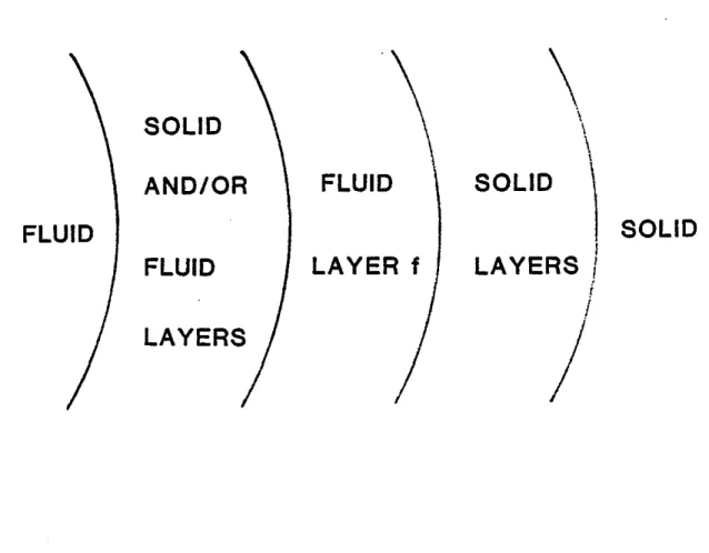
The model consists of a fluid cylinder surrounded by an arbitrary number of coaxial annuli (Figure 1). The annuli can be solid. such as the casing or cement; or fluid, such as drilling mud. The outermost. infinite layer is a solid. Each layer is homogeneous and isotropic. Complex layer parameters are used to incorporate attenuation into the calculations (Aki and Richards. 1980; Cheng et al .. 1982; Tubman et al.. 1984).

(

In layer n. the radial and axial displacements.u,. and v"' are given by: B9'" B?/In

u , . =

-Br Bz (1a) (lb) ( lc) (ld) (

where Pn. lI", and J.Ln are the density. Poisson's ratio, and shear modulus for layer n.

The scalar potential, 9'". and azimuthal component of the vector potential ?/In. are given by:

9'n

=

[A"

Ka(l"r)

+

A'" Ia(lnr)]e1l:(z-e')

?/I"

=

[B,.K1(m"r) +B'n I l(m"r)]e1l:(z-e.)

(2a) (2b)

where I_a.I,. K_{a• and} K1 are modified Bessel functions of the first and second

2-2

(

(3)

Unhanded Cased Holes 29

kind. c is the phase velocity and z the source-receiver separation. k is the axial component of the wave number and

z,.

and m.,. are the radial components of the P and S wave numbers.

An,

A'",B,., and B'" are constants for layer n.

Equations (1) can be written:

u;.(r)=D,.(r,,)(r)a,. where: and: (3) (4) (5)

D,.(r,,) is a .4%4 matrix whose terms are determined from substitution of equations (2) into equations (1). The elements of D,.(r,,) are given explicitly in Tubman

et at.

(1984).

It is necessary to relate the stresses and displacements in the o.utermost, infinite layer to those in the central lluid cylinder. In the case With all solid layers this expression is found to be (Tubman

et

at., 1984):

u,.

(rN_I)

=

_{DN_1}(rN-I)DN~l_{(rN-2)DN- 2(rN-2)' ..}l>:J-I(r I)U2(r I) (6) which can be re-written as

(7) where:

(8) The same formulation is used between the infinite formation and the outermost lluid layer that is used when all the layers are solid. Equation (7) cannot be extended to relate the displacement-stress vector across all the layers because not all components of the displacement-stress vector are continuous at a solid-lluid boundary. At the outermost lluid layer, the boundary conditions change and so the displacements and stresses can not be related across the boundaries in the same manner as before. The normal displacement, u, and normal stress, (J, are continuous. The tangential stress, "T, vanishes at the boundary. The tangential displacement, v, is discontinuous

because the solid and fiuid are free to slip along the interface.

The G matrix we have now can relate the displacement-stress vector inward only until the outermost fiuid layer (layer f). At that point the axial

(4)

30 Tubman etal.

(

(10) displacement is no longer continuous. Sb we now have

GaN

=

Uf+J(Tf) (9)

where Tf is the outer radius of layer

f

and uf+j is the displacement-stress vector in layer

f

+1.

Inside layer f, each boundary must be handled individually to allow for general geometries. Starting at the center and working out to layer f, the constants for each layer n, (a,,) , are written in terms of

a,

(which is just A',), Each layer may be either solid or fluid. This requires checking at each boundary to see it the next layer is a fluid or a solid. The type of boundary determines which components of the displacement-stress vector are continuous. This process yields the displacements and stresses in layer

f

in terms of those in the central fluid layer . .They are then matched to those in the next layer out (layer

f

+1). This completes the relationship from the infinite layer to the central cylinder. .

Dispersion Relation

The displacements and stresses have been related from the central fluid cylinder to the outermost fluid layer, (layer f). Application of the above results yields _Af and A'f in terms of A'" These are then used in equation (9) to complete the relation of the displacements and stresses from the central fluid cylinder to the outer, infinite formation,

Since there are no incoming waves in the outermost layer, A'N=B'N=O. In addition, A, =B, =0 so that the displacements and stresses remain tlnite atT =0.

B',=O as well because there is no vector potential in a fluid. Equation (9) is thus reduced to:

'Uf

(T/)

-Gil

-G13]

[A'I]

(Jf

h)

-G.1I

-~3

:t

=

0

o

G<I G43 N

This is the period equation for wave propagation in a borehole with a mixture of solid and flUid radial layers. Values of Ie and c for which this equation is satisfied yield the phase velocity dispersion relations.

Synthetic Microseismograms

In order to generate synthetic microseismograms it is necessary to include a source into the calculations. This is accomplished by imposing a boundary condition at T

"

the interface between the central tluid layer and the first annulus. The condition specified is an expression for a Ko(l,T) source in the frequency-wavenumber domain (Cheng at a.l., 1982; Tubman at a.l., 1984). This represents a point isotropic source on the borehole axis. The above calculations are then repeated in order to derive a relation similar to equation (10). This relation is used to solve for A' , which is then substituted into the form for the pressure response. In the time domain the pressure response. P.

inside the borehole is : (Tsang and Rader, 1979; Cheng at a.l .. 1982; Tubman at a.l., 1984):

2-4

(

(5)

Unbonded Cased Holes 31

-

.

(11)

-

-P(r,z,t) is the pressure response, Z the source-receiver separation. t time, and

X(",) the source spectrum. A'I is the only non-zero constant associated with the potentials in the central tluid cylinder. The excitation resulting from the Ko(IIr) source is added to the response function to give the total pressure tleld.

NUllERICALEXAMPLES

The geometries considered here have an intermediate tluid layer placed in one of two commonly occurring locations. The tlrst is between the pipe and the cement. This models the case of no pipe-cement bonding, or free pipe. The other geometry represents the case of poor cement-formation bonding. This is represented through the inclusion of a tluid layer 'between the cement and the formation.

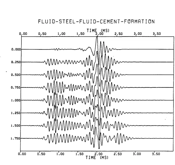
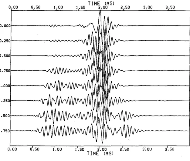
Figure 2 shows a number of microseismograms for the free pipe situation. All micro seismograms are for the same source-receiver separation, 10ft., and source, centered at 13 kHz. The source is the same as that used by Tubman et al .. (1984). The formation velocities are 13.12 ft/ms for Vp and 7.0 ft/ms for

V..

The dit!erence in the microseismograms of Figure 2 is the thickness of the tluid layer between the steel and the cement. The distance between the steel and the formation remains constant, so the cement thickness decreases as the tluid thickness increases. The tluid is replacing cement. The tlrst micro seismogram in Figure 2 has no tluid layer. This is the well bonded situation. The last waveform has no cement layer. The layers are just ones of tluid, steel, fluid, and the formation. Between these two extremes the thickness of the fluid layer increases in .25 inch increments (and the thickness of the cement layer decreases by this amount),

There is a large change in the character of the waveforms when the ll.uid layer in introduced. The microseismogram for the well bonded situation displays clear formation P wave and S wave arrivals. There is no distinct casing arrival. The additional tluid layer frees the pipe so the casing arrival is very obvious. The ringing from the steel completely obscures the formation arrival. Little change occurs in the waveforms as the thickness of the ll.uid layer increases. The casing arrival dominates throughout, although a slight increase in the amplitude and duration of this pipe signal may be observed as the ll.uid layer becomes larger.

Even a very thin ll.uid layer produces similar results. Tubman et al. (this report) show an example where the thickness of the ll.uid layer has been reduced to .001 inches in order to model a microannulus. The first arrival is from the casing despite the very small thickness of the ll.uid layer. Chang and Everhart (1983) showed the same ringing even at the limit of zero ll.uid thickness.

The important factor in determining the first arrival is whether or not the pipe is bonded to the cement. The thickness of the ll.uid layer between the steel and the cement has only a minor intluence on the character of the observed time series.

(6)

32

Tubman etal.

(

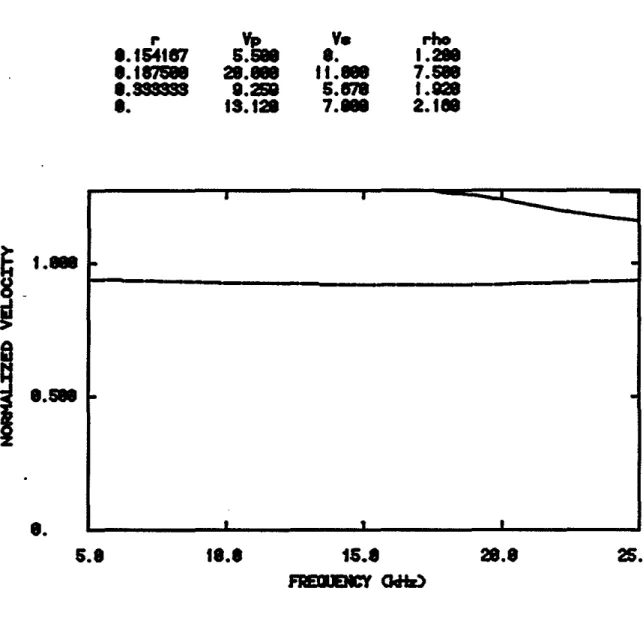
Dispersion curves corresponding to some of the microseismograms of Figure 2 are shown in Figures 3 to 6. The first one, Figure 3, gives the phase velocity dispersion relations for the well bonded cased hole situation. There are three distinct modes in the frequency range shown: the Stoneley and two for the pseudo-Rayleigh waves. (Only a small portion of the second pseudo-Rayleigh mode is seen.) The Stoneley wave is only slightly dispersive and is not cut off at low frequencies. The pseudo-Rayieigh curves are much more dispersive and are cut off at the shear velocity of the formation.

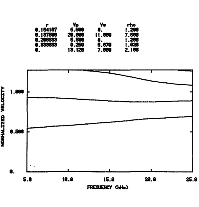
A fluid layer of thickness .25 inches has been inserted between the steel and the cement in Figure 4. As before, the thickness of the cement is .25 inches less. The pseudo-Rayleigh curves are shifted to lower frequencies than in the well bonded situation. The extra fluid layer could be causing an effect simllar to that produced by an increase in the borehole effective radius (Cheng and Toksoz, 1981). The Stoneley velocity is slightly lower at higher frequencies but the curve has not changed substantially. The interesting thing to note in Figure 4 is the presence of an additional Stoneley mode. This additional mode is due to the presence of the intermediate tl.uid layer between the steel and the cement. This mode has significantly lower velocity and is more dispersive than the one which was also observed in the well bonded situation.

In Figure 5 the thickness of the fluid layer is increased to 1.5 inches. The pseudo-Rayleigh curves have moved to still lower frequencies but the general shape of the curves has not changed. The flrst Stoneley mode has lower velocities in a small region about 20 kHz but the shift is not signiflcant. The second Stoneley mode has moved to much higher velocities. The Stoneley modes are now almost identical to those that observed in the case of no cement layer (Figure 6.)

The fluid layer has been decreased in thickness in Figure 7. This is the model of a microannulus. The fiuid layer has a thickness of only .001 inches. The pseudo-Rayleigh velocities have shifted back slightly to higher frequencies. The first Stoneley mode shows minor changes but the additional mode is now gone. The fiuid layer is now too thin to allow the propagaUon of the addition mode.

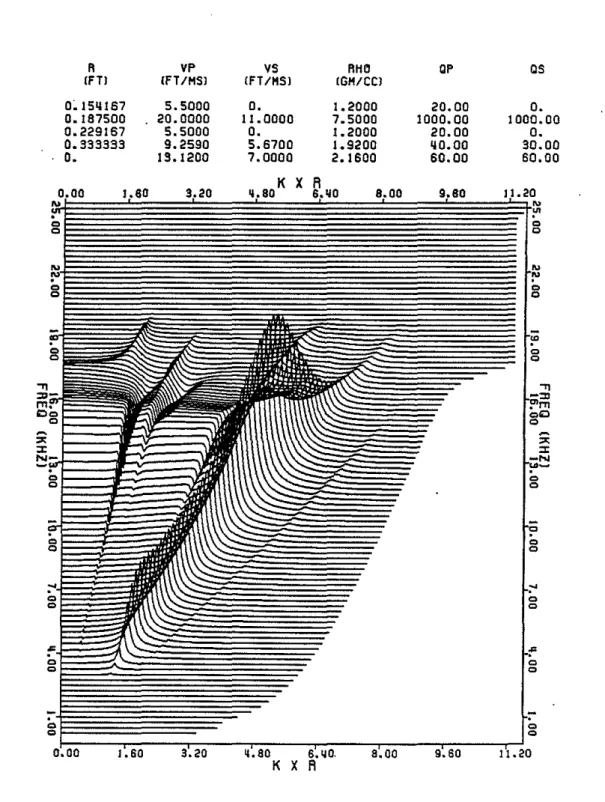
It is important to note that this additional Stoneley mode has not been observed in the microseismograms. This can be understood by looking at the frequency-wavenumber information (Figure 8). The arrival in question is the first encountered (counter-clockwise) from the kr axis. Clearly, there is very little energy associated with this wave. The power is not sufficient to be observable in the time domain. The fastest two arrivals are casing modes which were also observed by Chang and Everhart (1983).

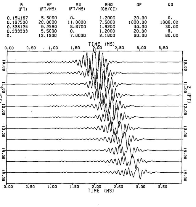
Figure 9 is the same as Figure 2 except that the intermediate fiuid layer is now located between the cement and the formation. Th first microseismogram has no Intermediate fiuid layer and the last has no cement layer. (These are the same waveforms shown in Figure 2.) Here it is clear that the character of the waveform changes as the thicknesses of the fluid and cement layers change. With the thick cement layer and thin fluid layer the formation arrival can still be distingUished. At the other extreme, with a thin cement layer and a thick fluid layer, the waveform has basically the same appearance as that in the free pipe situation. The first arrival varies as the amount of cement bonded to

2-6

c

( ( ( (

(7)

Unhanded Cased Holes ₃₃

the steel varies. This first arrival appears to be a signal due to the combination of the steel and the cement. A larger amount of cement damps out the ringing of the pipe decreasing the amplitude and duration of the first arrival. This same relationship between cement thickness and casing signal amplitude was observed by Walker (1968) in data from test wells with controlled bonding situations. The cement is also much slower than the steel. so increased influence on the velocity of the first arrival (due to the greater thickness)

results in a lower velocity. It should be noted that while the change in velocity I

of the first arrival is fairly clear in Figure 9, the cement velocity used is much less than the velocity of the steel. It the cement was faster, the change in velocity could be much less. The cement only influences the velocity of the first arrival to be less than that of the steel. The steel velocity still is the dominant factor.

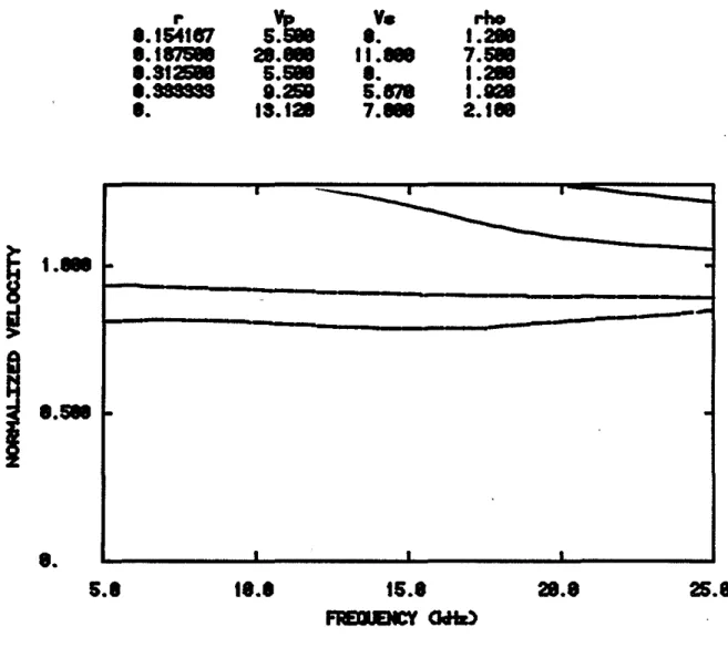
A thick cement layer bonded to the pipe is not sufficient to ensure that the formation arrival will be clear and distinct. Figures 10 and 11 have the same amount of cement (1.6875 inches) bonded to the pipe. The tluid layers are of different thicknesses though. The hole radius is larger in Figure 11 so that the fluid layer thickness is 1.25 inches compared with .0625 inches in Figure 10. While the formation signal is small in Figure 10, it is clear and able to be distinguished. The first arrival in Figure 11 is more obscure and difficult to identify.

Figures 12 to 14 show similar behavior for the dispersion curves as in the free pipe situation. A thicker intermediate tluid layer shifts the pseudo-Rayleigh dispersion curves to lower frequencies relative to the thin layer (Figures 12 and 13). The primary Stoneley mode changes only slightly and the additional Stoneley mode has significantly higher velocity with the thicker fluid layer. Again. the second Stoneley mode disappears completely when the thickness of the tluid layer is very small (Figure 14). A thick fluid layer yields curves that are virtually the same as those with no cement layer. Much more study is warranted on the nature of this additional Stoneley mode.

CONCLUSIONS

A formulation has been developed for the phase velocity dispersion relations and impulse response of radially layered cylindrical geometries including intermediate fluid layers. Examples are given for a number of situations encountered in poorly bonded cased boreholes. It is found that in the case of a free pipe, (with a fluid layer between the steel and the cement), the presence of the fluid layer is the most important factor in determining the nature of the microseismogram and what will be the first arrival. The thickness of the layer has only minor effects. It there is good pipe-cement bond but no cement-formation bond the thickness of the fluid layer as well as that of the cement layer become important. A thick layer of cement bonded to the steel can damp out the ringing of the casing arrival making it possible to identify the formation arrivals. It the cement layer is thinner, the first arrival will be from a combination of the steel and the cement.

A second Stoneley mode is shown to exist in the presence of an intermediate fluid layer of sufficient thickness. The nature of this wave is most dependent upon the parameters of the fluid layer. The additional Stoneley

(8)

34 _{Tubman et al.}

(

mode is found to have only a small amount of energy and so does not contribute significantly to observed microseismograms. More study is required to fully understand the propagation of this additional mode.

ACKNOWLEDGEllENTS

This work was supported by the Full Wavl!form Acoustic Logging Consortium at M.LT. Kenneth Tubman was partially supported by a Phillips Petroleum Company Fellowship. 2-8 ( ( ( ( ( ( (

(9)

Unbonded Cased Holes

REFERENCES

35

Aki, K and Richards, P., 1980, Quantitative Seismology Theory and Methods: v.I., San Francisco, W.H. Freeman and Co.

Baker, L.J., 1981, The etrect of the invaded zone in full waveform acoustic logging: 51st Annual International SEG Meeting, Los Angeles, CA.

Chan, A.K and Tsang, L., 1983, Pl'opagation of acoustic waves in a fluid-filled borehole surrounded by a concentrically layered transversely isotropic formation: J. Acoust. Soc. Am" 74, 1605-1616

Chang, S.K and Everhart, A.H., 1983, A study of sonic logging in a cased borehole: J. Pet. Tech., v.35., p.1745-1750.

Cheng, C.H. and Toksoz, M.N., 1981. Elastic wave propagation in a fluid-filled borehole and synthetic acoustic logs: Geophysics, v.46., p.l042-1053.

Cheng, C.H., Tubman, KM., and Toksoz, M.N., 1981, Propagation of seismic waves in a multilayered borehole: 51st Annual International SEG Meeting, Los Angeles, CA.

Cheng, C.H., Toksoz, M.N., and Willis, M.E., 1982, Determination of in situ attenuation from full waveform acoustic logs: J. Geophys. Res., v.87.,

p.5477-5484. .

Cole, S.P., 1983, Guided wave dispersion in a borehole containing multiple fluid layers, B.S. Thesis, Department of Physics, Massachusetts Institute of Technology, Cambridge, MA.

Schoenberg, M., Marzetta, T., Aron, J., and Porter, Ro, 1981, Space-time dependence of acoustic waves in a borehole: J. Acoust. Soc. Am., v.70., p.1496-1507.

Tubman, KM., Cheng, C.H" and ToksCiz, M.N., 1984, Synthetic full waveform acoustic logs in cased boreholes: Geophysics, in press.

Walker, T., 1968, A full-wave display of acoustic signal in cased holes: J. Pet. Tech., p.818-824.

(10)

36 _{Tubman etaL}

APPENDIX

(

( This appendix gives the details ot the calculations tor each type ot

interface. The constants

An,

A'n' ~ and B'n are found in terms of the constants in the next layer inward (layer ... -1). These are in turn expressed in terms otA'I and possibly

An

from an inner layer. These are the constants that determine the potentials tor the layers. The relationships between these terms are expressed using two sets ot constants: a.; and c" These constants have no particular physical meaning. They are used only to keep the derived expressions manageable, The results ot each ot the following sections can be used 'as the starting point tor another section it turther calculations are required,

Fluid-Solid Boundary

Let layer ... be the tluid layer and layer ...

+

1 the solid, The boundary is then at rn , The boundary conditions are continuity ot radial displacement and stress and zero axial stress, The axial displacement can be discontinuous,

u,,(rn ) =u,,+1(rn) (Ala)

(

(Alb) (Ale) In the tluid layer there are two constant terms,

An

and A'n. It is assumed that these are both expressed in terms ot

A\,

Shortly, it will be clear that this is always the case, _{The solid has tour constants: An+I, A'n+',} B_n+_{I ,} and

Ii

n+l' There are three equations, then, and five constants to be determined. A'n+I'

Bn +" and B'n+l are found in terms of An+1 and A'I' .

The equation for continuity of normal stress (equation Ala) can be written explicitly as:

Dn +l u An+1+D,,+112A'n+1 +Dn+11.Ei. +1+D,.+11o

B

'n+1=DnuAn +Dnl.A'n (A2)

where,

An

and A'n are both in terms ot A'I:

An

=

CloA'1 A'n _{=Cl IA'1}

a.; are constants, Substituting into equation (A2) yields:

Dn +1 u An +1 +Dn +112A'n +1 +Dn +11.Ei.+1 +D,. +lIOB'n+I=(D"IIClo+Dn,.ClI)A', (AS)

In a similar manner, the continuity of normal stress (equation Al b) can be written:

D,. +l31An+1 +Dn +13.A'n+' +Dn +133

Ei.

+1 +D,.+I ..B'n +1

=

(Dn uClo+Dn,.ClI)A', (A4)

and zero tangential stress at the boundary (equation Ale) can be written as: D,.+1..An+1+D,,+1_o•A'n+l_{+D,.+1o.Ei.+l +Dn+1..B'n+,}=0 (A5)

2-10

(

(11)

Unbonded Cased Holes

A setof constants Cj is defined to simplify notation, Let: Co = ])"uao+Dn,.a I

A'n+1 can be eliminated from equations (A3) and (A5) , This yields: C2A"+1 +cs.8,,+,+C4B'n+1=coA', where: 37 (A6) ]),,+'I.Dn+'.. C4

=

]),,+'" ]),,+1••

Similarly, A'n+1 can also be eliminated from equations (A4) and (A5) to give:

c~A"+1 +C e.8" +1 +C7Bn+' = cIA', (A7)

where: Dn.+1 3aDn+143 Dn+1...₂ ]),,+13•Dn+l . . c7= ])".,,.- n .I""'n+l..2

Bn +, can now be eliminated from (A6) and (A7) to give and expression for B'n+'

interms of A,,+1 andA',:

B'n.,=ceAn+l+cgA', (AS)

(12)

Tubman et aL 38

Substituting equation (AB) into equation (A7):

0~"+1+06.t;.+1 +07( osA,.>\+0gA'">\)

=

0 IA'I

Solving tor.t;. +1 yields:

(A9) where:

SUbstituting equation (AB) and equation (A9) into equation (AB) yields: D,.,+I.,A,.+I+D,.>\..+D,.>\••(olOA,. +1 +0 !lA'I)+D,. >\..(0 sA,.+1 +0 gA 'I)

=

a

Which can be solved to find and expression torA',,+I in termsot A,.+1 and A'I:

A',,+1=012An>\+0ISA'1 (Ala)

where:

Equations (Ala), (A9), and (AB) then give A'n+I' .t;.+I' and B'n+l in terms ot A'I

and A,.>\,

Solid-Fluid Boundary

The solid, layer n, has constants An, A'n' .t;., and B'", all expressed in terms of A'I and A,. (or A trom some inner solid layer). The fiuid, layer n +1. has constants An+1 and A',,>\. The boundary conditions are the same as in the

previous case ot a solid-fiuid boundary. A,. and A'n are determined in terms of

A'I' The continuityot radial displacement is written as:

D_{n + lll}An>\ +D,. >\12A'n+1

=

0 16A,. +017A'1 (All)

where:

2-12

(13)

Unbonded Cased Holes

e17

=

Dnuc115+Dn12c lS+Dn13c 11 +Dn1.cg

The continuity of radial stress gives:

)),,+'31A,,+,+D,._{+1 32A'n+'} =c ,eA" +c,gA', where:

39

(A12)

The condition that the axial stress must vanish at the interface is written explicitly as:

where:

02'=Dn.,o ,.+Dn•₂₀,s+Dn•₃cII+))"••Cg

A" is ellminated from equation (All) and (A13). The result is:

D,.+'uA"+1 +Dn+"2A'n+1

=

022A',

where:

cleC 21

C22=017-°20

Similarly eliminatingA" from equations (A12) and (A13) yields: D,.+131An+,+!l,.+'32A'n+1=°2SA',

where:

A'nH is then eliminated from equations (A14) and (A15), The result is: An+1

=

aoA', where: (A13) (A14) (A15) (AlB)

(14)

40 _{Tubman et}_aI.

Substituting equation (AlB) into equation (A14) yields:

A'n+1

=

a,A',

where:

(Al?)

If this fluid layer is the outermost fluid layer, (layer!), the displacements and stresses are now related across all the layers. Otherwise, the results of this solid-fluid case can serve as input for the fluid-solid boundary conditions if the next layern+2 is a solid. (Recall that the constants ao and a1were used earlier

in the case of a fluid-solid boundary.)

Solid-Solid Boundary

In the inner solid n, there are four constants An, A'n' .8,., and B'n' all of which are expressed in terms of An andA'I' The outer solid has constants An+1' A'n+I' Bn+1' and B'n+1' The boundary 'conditions at Tn are the continuity of

radial and axial displacements and stresses:

... (Tn ) = ... +I(Tn ) (AlBa)

Vn(Tn ) =Vn+I(Tn )

ern(Tn)

=

ern+l(rn ) 'T"n(rn ) ='T"n+1(rn )

An+I' A'n+1> .8,.+1' and B'n+1 will be found in terms ofA'I and An.

(AlBb) (Al8c) (AlBd)

(

If there are several solid layers together in a group, this section is used repeatedly, determining all constants in terms of A'I and ~, where i is the innermost layer of the group. All four components of the displacement-stress vector are continuous across Tn' the interface between the two solid layers n and n+l. Thus:

or

2-14

(15)

Rearranging:

Unhonded Cased Holes

41

(A19) layer) .

(A20)

Equation (A20) gives .4,.+1' A'"+1' ~+I' and B'''+1 in terms of .4,. and A'I' The results can be put into the form:

.4,.+1

=

c 1..,4,. +cI~A'1

where the constants c, do not have the same values as in equation (A20). They are new values determined by the matrix multiplication. The reason for using the same terms is that if the next layer (n+2) is also solid, these new values are substituted directly into equation (A20) to continue through all solid layers.

Fluid-Fluid Boundary

The inner tluid, layern, has constants A" and A'". both in terms of A'I' The outer tluid has constants .4,.+1 and A'''+I' The boundary conditions are the continuity of radial displacement and stress:

u,,(rn )

=

u,,+1_{(rn )} (A21a)

a" (r,,) =a,,+l(rn ) (A21b)

The inner tluid has constants An and A''1 which are both known in terms of A'I' The outer tluid has constants .4,.+1 and A "+1'

. The continuity of radial displacement (equation A21a) can be written explicitly as:

The continuity of radial stress (equation A21b) is:

A'I(aoD,.., +a lD,. ..)

=

D"+1.,.4,. +1

+

D"+I,.A·n+1

A'n+1 is eliminated from equations (A22) and (A23) to yield;

(A22)

(16)

42 where Tubman et aL ,4,,+1

=

a'oA'1 (A24) (AZ5) ( (

A'n":l is determined by substituting equation (AZ4) into equation(A2Z) , The result is:

(A26) where:

(A27) (

a'o anda'i replace ao and a_l iffurther calculations are required,

2-16

(

(17)

\

SOLID

\\

\

ANDIOR

FLUID

SOLID

I

FLUID

SOLID

I

FLUID

LAYER f

LAYERS

I

,

t

LAYERS

)

Fig. 1. Geometry of the model. The first layer, the central fluid cylinder, is fluid. The outer, infinite layer is solid. The intermediate layers can be either solid or fluid. The outermost tluid layer is labeled layer! .

(18)

(

44

_{Tubman et}_aL ( ( 3.50 3.00 1.00 0.50 FLUIO-STEEL-FLUIO-CEMENT-F~RMRTIDN TIME (MS) 1.50 2.00 2.50 0.00

o.oool---"\I\r---"-\,../

0.2501----""\J\ 0.5001---~N\

o.

7501---~..J\1 I.oool---~N\ I.2501---~VI/\. I.5001---~N\ 1 •7501---~._./\ ( ( 0.00 0.50 1.00 1.50 2.00 2.50 TIME (MS) 3.00 3.50 (

Fig. 2. Microseismograms for various thicknesses of the tluid layer between the steel and the cement. This is the free pipe situation. The source-receiver separation is 10ft. The source center frequency is 13 kHz. The tluid layer thickness increases in .25 inch increments. The cement layer thickness de-creases by this amount. The first microseismogram has no tluid layer (the well bonded case) and the last has no cement layer. The P velocity of the formation is 13.12 ft/ms and the S velocity is 7.0 ft/ms.

(19)

..

1.1S4187

1.1'"

I.SSSSSS

I. s~

28.B

8.B

IS. 128

• v.

I. II.B

5.178

7.8

• rho

I._

7.S88

I._

2.1.

v·

r " - - - . , "

1.- "

e.

5.1

•

11.1

•

• 28.e

.

25.8

Fig. 3. Phase velocity dispersion curves for the well bonded situation. The velo-cities are normalized to the borehole fluid velocity. The Stone ley mode (dashed line) and two modes of the pseudo-Rayleigh (solid lines) are present in this fre-quency range.

(20)

46 Tubman etal. (

•••

••

,.

s~

v.

rho

•. tS4t87

••

1.288 '.t""

28....

II ....

7. •

'.211!95

5. •

••

1.288 '.9BB!!!

•••

s.m

1 .

-••

18. t211

7....

2. tee

,

\

•

~

.

~

.

I

,

•

5.1 tl.1

tS.1

fRECIENC'( CJdiK)

28.1

25.1

Fig. 4. Phase velocity dispersion curves for the free pipe situation where the fiuid iayer between the steel and the cement is .25 inches.

(21)

Unbonded Cased Holes

,.

S~

v.

rho

1.154187

I.

1.288 1.111 31

28.B

II.B

7.588 1.812511

5.588

I.

1.288 I.sssns

IUD

5.8'18

1.128

I. IS.I28

7.B

2.1.

47

1.588

I.

I I I

-l-

.

• •

•

5.1

11.1

15.1 FREllEIEY

Ocfk)

28.8

25.8

Fig. 5. Phase velocity dispersion curves for the free pipe situation where the flUid layer between the steel and the cement is 1.5 inches.

(22)

48 Tubman et al. I"

8.154187

'.187588

'.SSSUS

I. s\.

28."

5. •

13.128 v.

I. I I . "

8. 7."

rho

I . •

7. •

I . .

2.188

(

8.

I I

-

.

l-

.

• • •

5.'

18.8

15.8 fREllENCY

CWfz)

28.8

25.8

(

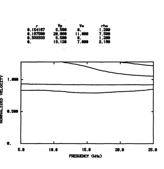
Fig. 6. Phase velocity dispersion curves for the free pipe situation. There is no cement layer between the steel and the formation.

(23)

Unbonded Cased Holes r

5~

v.

rho

'.154187

••

I . •

'.1""

•••

II . •

7. •

I.Ilmi8S

5. •

I .

I . •

I.SlS!!!

•••

5.m

I . •

I. IS.I.

7. •

2.1.

•

49

1'0.

II-- - - -

~.

I . . . .

••

5.'

• II.'

• IS.'

f1lFlIJEIK:Y

CWta)

• 28.'

.

25.8

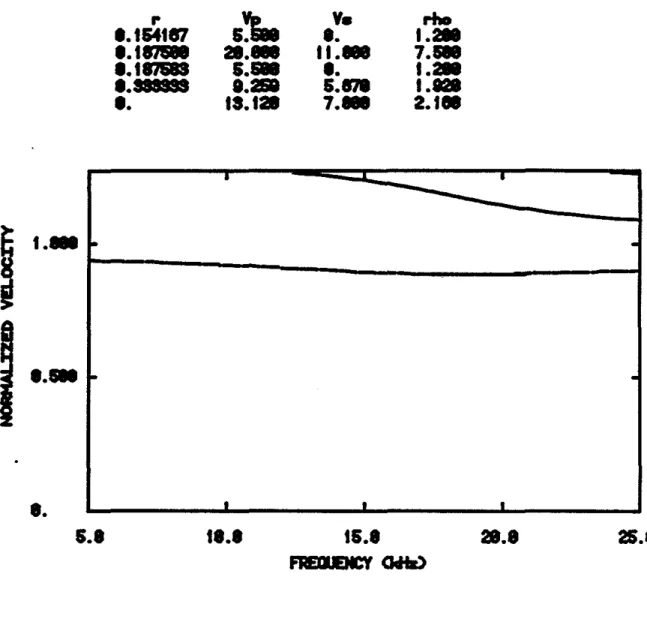
Fig. 7. Phase velocity dispersion curves for the case of a micro annulus. The thickness of the fluid layer between the steel and the cement is .001 inches.

(24)

50 _{Tubman et}_aL R VP V5 RHO OP OS IFTl 1FT1/151 1FT 11151 IG/1/CCI 0~15~167 5.5000 O. 1.2000 20.00 O. 0.187500 20.0000 11.0000 7.5000 1000.00 1000.00 0.229167 5.5000 O. 1.2000 20.00 O. 0.333333 9.2590 5.6700 1.9200 ~o.oo 30.00 O. 13.1200 7.0000 2.1600 60.00 60.00 K X R 9.80 11.20 0.00 1.80 3.20 ~.80 6.ijO 8.00 N

'"

:n

..

N N ( ~ ~ 8 C> c ~

..

;:

::J: ::J: N-

.

-N

..

(

..

;,

..

~ _:-'

..

1" 1"

..

c c 0.00 1.60 3.20 ~.80 6.~0. K X R 8.00 9.60

..

1l.20

Fig. 8. Magnitude of the frequency-wavenumber spectrum for a free pipe situa-tion. The spectrum has been multiplied by the source funcsitua-tion. The fluid layer between the steel and the cement has a thickness of .5 inches.

(25)

Unbonded Cased Holes 51 3.50 3.00 1.00 0.50 FLUID-STEEL-CEMENT-FLUID-F~RMATION TIME (MSl 1.50 2.00 2.50 0.00 O.OOOI---'V\I'-'~---"I."VO/ O.250'f---~""'1'v-~..."N""\ 0.500f---v'\/V'-vv..N\ 0 . 7 5 0 f - - - V \ ) 1 . 0 0 0 1 - - - . ) 1.2501f---"\ 1.5001---~W\ 1.750f----...,[I,J 0.00 0.50 1.00 1.50 2.00 2.50 TIME (MSl 3.00 3.50

Fig. 9. Microseismograrns for various thicknesses of the fluid layer between the cement and the formation. The fluid layer thickness increases in .25 inch in-crements. The cement layer thickness decreases by this amount. The first mi-croseismogram has no fluid layer (the well bonded case) and the last has no ce-ment layer. The P velocity of the formation is 13.12 fUms and the S velocity is 7.0 fUms.

(26)

(

52 Tubman etaL

,

\

R VP VS RHO OP

as

efT) .IFT IMS) 1FT IMSJ eGM/CCl

0.154167 5.5000

O.

1.2000 20.00

O.

0.187500 20.0000 11.0000 7.5000 1000.00 1000.00 ( 0.328125 9.2590 5.6700 1.9200 40.00 30.00 0.333333 5.5000

O.

1.2000 20.00

O.

13.1200 7.0000 2.1600 60.00 60.00

TIME eMS)

0.00 0.50 I. 00 1.50 .00 2.50 3.00 3.50 ( co co co c co co

--

( N ' _{• N} co co co co -n -n -< -< rio>

·

co c c c (

...

·

co c c co (

'"

c co co c PI c c c c 0.00 0.50 1.00 1.50 2.00 2.50 3.00 3.50

TIME (MS)

Fig. 10. Microseismograms for a case of good steel-cement bond but no cement-formation bond. The cement thickness is 1.6875 inches and the fluid thickness is.0625.

(27)

R

VP VS

RHO

ClP CIS

eFT) eFTIMS) 1FTIMS) eGM/CC)

0.154167 5.5000

O.

1.2000 20.00

O.

0.187500 20.0000 11. 0000 7.5000 1000.00 1000.00 0.328125 9.2590 5.6700 1. 9200 40.00 30.00 0.432267 5.5000 O. 1.2000 20.00

O.

13.1200 7.0000 2.1600 60.00 60.00 TIM (MS) 0.00 0.50 1.00 1.50 0 2.50 3.00 3.50 c

.

c c <> c N~ ' N c c c c

"

- i - i

"

'"

·

<>

.

c c c

·

:-" c c c c

"

·

c c c c

·

~ c c c c 0.00 0.50 1.00 1.50 2.00 2.50 3.00 3.50

TJ

ME (MS)

Fig. 11. Microseismograrns lor a case 01 good steel-cement bond but no cement-formation bond. The cement thickness is the same as in Figure 10, but here the hole radius is larger so the flUid layer between the cement and the for-mation has a thickness of 1.25 inches.

(28)

54 Tubman etaI. ( r

S~

v.

rho

I. t54t87

I. I.-

_e

•. t87S88

28._

It._

7.S88

'.St2SB8

8._

5.878 1.-•. sssns

S.S88

I. 1.-••

tS. t28

7._

2.t •

(

I···

8.

•

• -

.

r

.

•

(

5.8 t•••

tS.'

FRErIENCY

GIHz)

28.8

25.8

Fig. 12. Phase velocity dispersion curves for the case of good steel-cement bond but no cement-formation bond. The tluid layer thickness is .25 inches.

2-28

(29)

55 Unbonded Cased Holes

r

S~

v.

rho

'.154187

••

I . •

1.1878

a . •

II . •

7. •

1.211m

I.B

s.m

1._

'.SSUU

5. •

••

I . •

I.

11.121 7. •

2.1111

•

io _•

•

• I . •

I. 5.'

I'.'

IS.'

FRmJEIICY

CkItI)

28.'

25.8

Fig, 13, Phase velocity dispersion curves for the case of good steel-cement bond but no cement-formation bond, The fluid layer thickness is 1.5 inches,

(30)

56 Tubman etaL r

s\.

v.

rho

1.154187

I. t._

_t

1.117SlI8

21._

_11.-

7.AI