Design and construction of a SIMKIT analog computer with remote control

DESIGN AND CONSTRUCTION OF A SIMKIT ANALOG COMPUTER WITH REMOTE CONTROL

by

ROBERT L MARESCA

Submitted to the Department of Mechanical Engineering

on May 12, 1978 in partial fulfillment of the requirements for the Degree of Bachelor of Science.

ABSTRACT

This thesis concerns the construction of a system (SIMKIT) which through analog computation simulates a certain ecodynamic model. The purpose of the SIMKIT

is to explore the stability boundary for a certain range of input parameters. Sonar remote control is used to address different nodes in the circuit and to vary critical parameters from a distance.

Thesis Supervisor: Title:

Henry M. Paynter

TABLE OF CONTENTS

PAGE ACT

GENERAL INTRODUCTION.

INTRODUCTION TO THE SYSTEM PROBLEM THE DESIGN PROCESS

A. Analog. B. Digital.

HOW TO USE THE SIMKIT CONCLUSION

2

I. INTRODUCTION

The use of analog computation has all but disappeared with the onset of the digital computer. Present day

digital computers are more accurate and certainly more practical than the analog computers of the 50's. Never-theless, the same technology which advanced the digital computer so far (ie. integrated circuit technology) has also cast a new light on analog simulation. Function blocks (eg summers, integrators, etc.) can be made from op-amps costing as little as 50 cents. Multipliers can be made using the logarithmic characteristics of the bipolar transistor; and dividers and other non-linear

circuits can also be synthesized relatively inexpensively. The analog computer is very useful as a learning

tool. _{Inputs are generally determined by pots which} allows the experimenter to adjust parameters manually

and observe the effects on the system. This gives the student a real "feel" for the effect of each input on the system.

This can be reinforced with regard to stability problems by the inclusion of audio circuits to indicate instability.

In this particular paper, the process of designing and building an analog computer, which will be referred to as a "SIMKIT", is explained and documented. The

system which is being simulated is a model of an ecodynamic system, the Quinlan-Paynter rudimentary element cycle

model. (I)The model is a third ordcr system described by 3 non-linear first order differential equations(2) which predict a straight line stability boundary.

The object of this particular SIMKIT is to make clear the effect of certain parameters on tie stability of the system. By changing two parameters while holding all others constant, we can trace out the stability

boundary which separates the system parameter space into two distinct regions: one being stable and the other allowing limit cycles.

This SIMKIT is not restricted to representing only this system. Wiring has been done on easily alterable terminal strips which allows the user to generate his own functions and synthesize many systems. The features of the SIMKIT include: an audio circuit which detects ac signals in the audio range; a remote control channel

which allows the user to address any one of five different node voltages and have it displayed on a voltmeter; and

(1) _{As proposed in STABILITY OF AN ECODYNAMIC SYSTEM by} Alician Quinlan and Henry M. Paynter, 17 June' 1977. (2) _{Some-Simple Non-linear Dynamic Models of Interacting}

Element Cycles in Aquatic Ecosystems, A.V. Quinlan, H. M. Paynter, (An ASME Publication, Paper No.

a second remote control channel which enables the user to control two different node voltages, presumably input parameters.

These basic features enable the SIR-KIT to adequately handle many system models of similar complexity to the ecodynamic system; furthermore, additional remote controls and terminal strips may be added in the future to provide even more flexibility of operation.

II. INTRODUCTION TO THE SYSTEM PROBLEM

The ecodynamic system model being simulated on the SIMKIT is a rudimentary element cycle model as

proposed by Quinlan and Paynter.(3) The model includes three variables which represent the mass of a chemical element stored in plants (X), animals (Y), and minerals

(Z). The total mass, M , of the element in the system is constant (.* X + Y + Z = M). M is a system parameter which along with five other parameters define the

system. These other parameters characterize the three basic matter flows required for element cycling (they are: uptake, predation and remineralization).

The system equations are given below along with a schematic representation of mass flows in the closed system.

The mass flow rates (RZX , RXY , RYZ) all exhibit linear behavior through rate constants, a , b , and c, respectively; while the uptake and predation rates also

Z

exhibit saturation characteristics modelled by Z+A and

X

, respectively. Intuitively, these rates laws, though a simplification of a biogeochemical process, do indeed make sense. One would expect the rate of predation to be a function of the number of predators (the number being

related to the magnitude of Y) and therefore the expression:

PLANT

x

ANIMA L

r=a tRYZ=cY

=Rzx-RXy

Rxy-cY

)

Z=M-X-Y

(3)

Figure 1: Schematic of Mass Flows in Ecodynamic System - Along with System Equations.

MlY c bY. One would also expect the uptake rate to be related to the amount of food available unless the food is so abundant that any increase in food supply would, have no effect on the rate of uptake because the predators can only eat a limited amount. This is a saturation

X

phenomenon and is modelled using the term y _x+B , in the

rate law,

flY- bY

_X+B

This equation indicates that

as X gets large compared to B , the rate law reduces to RXY = bY which is independent of X and thus provides a representation of saturation in food supply. The reader should convince himself that the other two rate laws RZX and RYZ are equally intuitive and thus constitute a reasonable model for this system.

The three equations which describe the system are shown in Figure 1 (eqs. 1, 2 and 3). It has been found that the system has a stability boundary which separates its parameter space into 2 regions: one, allowing damped returns to equilibrium and the other permitting limit cycles. (3) This stability boundary is a straight line in each of the three 2 dimensional parameter spaces. Each line represents a locus of parameter conditions which

satifies the stability limit, ie.

a=' t(aA/bY) - (B+X)/(A+Z) = 1, where X , Y , Z represent equilibrium values.

The linear stability boundary in any parameter space can be derived using the above equation along with the equilibrium conditions:

The stability boundary was discovered by Quinlan and Paynter (1975, 1976).

a ( )-b ( )=0 (1a)

Z+A X+B

b X ) C 0(2a) X+B

X + Y + Z =M (3a)

For example, the straight line boundary which exists in the X-Y parameter space is found through suitable

algebraic manipulation to be

a b a -b))X a a b

Yc = - (- (1+-)/(- - )) Xc + c/(c - -)) M. (4)

c c c c

c

Equation 4 along with the constant mass equation (X + Y + Z = M) can be plotted in the X-Y parameter

space to show the two distinct dynamic regions (Figure 2). If the parameters of the system are such that it is in region 1 then it will exhibit limit cycles. If the system parameters are such that the system operates in region 2 then it exhibits damped returns to equilibrium.

Similar algebraic manipulation leads to straight line stability boundaries for the other two parameter

spaces. one can also draw the three dimensional parameter space where the stability surface divides a tetrahedron

(see Figure 3) into an unstable volume and a stable volume. In comparing these two volumes, one can answer questions

a/c 1+ a/c Figure 2. -

b~1

I

X+Y=M

2

UNSTABLE STABLE

x

Stability Boundary in X-Y Parameter Space

such as, what is the probability of stable behavior given a randomly picked equilibrium coordinate (X , Y , Z); or, given a set of saturation parameters, A and B, how may one choose a , b , and c to guarantee limit cycles or

equilibrium behavior. These questions and others like them concerning the stability of a system are often encountered in environmental engineering problems related to aquaculture, agriculture, and bioaccumulation of toxic substances.

Stability

Boundary

_Unstable

(Surf~zeVolume

Stable Volume

Figure 3. X , Y , Z parameter Space with Stability Surface

Thus, this system has been chosen to be the one simulated on the SIMKIT with manual adjustments for M , a , b , and c and Remote Control adjustments for A and

III. THE DESIGN PROCESS

The design process can be broken up into two distinct stages: first, is the analog circuit design to simulate

a given set of system equations; and second, is the digital design which is responsible for the remote

control variation of parameters along with a multistation addressing function.

The objective is to design an electrical system which behaves like a jiven ecodynamic system described by the following equations:

z

X = aX (-) - bY(L) (1)

X

Y= bY (X-) - cY (2)

Z= H- (X+Y) (3)

From these equations, it is evident that the system is non-linear and thus will require some non-linear function blocks (eg. dividers and multipliers). The system variables

are X , Y, and Z; while the parameters are a , b , c ,M, A , and B which are all time invariant. Thus, any

multiplication of variables will require a multiplier

a divider (x+B -) Therefore, 2 multipliers and 2 dividers are needed. Furthermore, the two derivatives, X and Y, indicate that 2 integrators are needed.

The fact that the system parameters are time

invariant implies that potentiometers may be used to generate these parameters; and with the addition of a few summers, one has all he needs to model the system.

A convenient way to synthesize the necessary analog

functions is to start by assuming that X and Y have already been generated and proceed to build the other function

blocks using X and Y as given.

Let the starting point be equation 3. This calls for a summer which can be made from an op-amp

(Figure 4). In generating Z , one must first generate -M by means of a pot from -Vcc to ground. The resistance of the pot should be small compared to the summing resistors

to insure against loading effects. Also, a 250K resistor is connected to the non-inverting terminal of the op-amp to minimize erros due to bias currents which are on the order of .lzA. Better op-amps could be used (eg CMOS op amps, CA3140's); however, the 741 comes in a 14 pin Quad chip which makes for more efficient use of space and

as in Figure 4 , one can expect an accuracy of about 1% which is less than the error introduced by tolerances in resistor values. All summers in the system are constructed using the below configuration and all pots are restricted to be 10K.

.Vcc

50

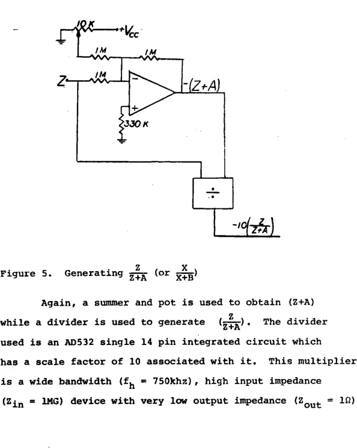
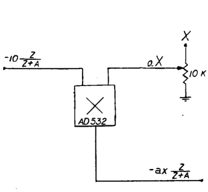
Having generated Z , one can now proceed to generate Z/(Z+A) as shown below in Figure 5.

c

/M//

-S

z x

Figure 5. Generating (or B)

Again, a summer and pot is used to obtain (Z+A)

Z

while a divider is used to generate (-) The divider used is an AD532 single 14 pin integrated circuit which

has a scale factor of 10 associated with it. This multiplier is a wide bandwidth (fh = 750khz), high input impedance

it is for all practical purposes a unidirectional device which behaves as an ideal function block. The divider is accurate to within 4% for inputs between 1 and 1OV.

The drawbacks of this device are that it is

expensive ($36.00/1977) and has much better performance than is needed for this application. One might consider building a divider out of 4 op-amps and 2 transistors, making use of the log characteristics of the transistor. This would take up more space but would be much cheaper

($4.00/1977) and would probably serve just as well in

this application. Nevertheless, four AD532's were used: two as dividers and two as multipliers.

X

The method of generating XB is exactly the same Z

as that for

The next step is to synthesize bY (-) and aX (snX+B

x

Z

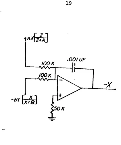
All that remains now are the integrators. To generate X , one must integrate equation 1 as shown in Figure 7.

.00/UF

/00 K

-bY

OK

Figure 7. Generating X by Integrating Equation 1. A similar circuit generates Y as shown in Figure 8.

Now, all the tens of the equation have been generated and all that remains is to connect each function block

(Figures 4-+ 8) to simulate the entire system. A complete circuit diagram is shown in Figure 9 with various nodes

marked indicating the functions of each part of the circuit. Note that the resistors are left off the non-inverting

terminals for sake of clarity and all resistors are 1MEG unless otherwise marked.

Figure 8. +13 100K .00/ UF 00K] 50 K cy ~I U Ux

Generating Y by Integrating Equation 2.

Once the analog computer has been designed, all that remains is the construction or wiring of the circuit. The circuit was built on easy plug in terminal strips

which prevented the need for soldering and greatly facilitated trouble shooting. The construction process is best

described as a series of 13 steps with a functional check after each check.

+ I r) NC

AL

-1

I1

Figure 9. Complete Analog CKT Diagram.

4

4 4

41

To start, X and Y are generated as 4 Volts while M = 10V , A=B=3V, and a=b=c=.2.

STEP 1 Generate Z; check Z=2V

STEP 2 - Generate -(Z+A); check -(Z+A)= -5V STEP 3 - Generate - Z+A ;check - (Z) = -4V

Z+ Z

STEP 4 - Generate -aXZ (=); check -aX(Z+A

STEP 5 - Connect -aX( ----) to X integrator STEP 6 - Generate -(X+B); check -(X+B)= -7V

STEP 7 - Generate -X( ); check -(----) = -5.7V

Xi- X+

STEP 8 - Generate - bY(-): check -bY(-) = -. 46V STEP 9 - Connect -bY(-) to X integrator

X+

STEP 10 - Generate +bY(-) and connect to Y integrator

STEP 11 - Generate cY; check cY = .8

STEP 12 - Connect cY to Y integrator

STEP 13 - 1isconnect 4V generator for X and Y and replace them with the output of the

2 respective integrators. Check X+Y+Z = 1OV. After finishing the 13 steps, the circuit is complete. To make sure the circuit is behaving as it should, set

a=.4 , b=.2 , c=.l , A=4.OV , B=2.OV and M = 1OV. The

system should. be unstable for these values and any variable X , Y , or Z displayed on a scope should exhibit limit cycle behavior.

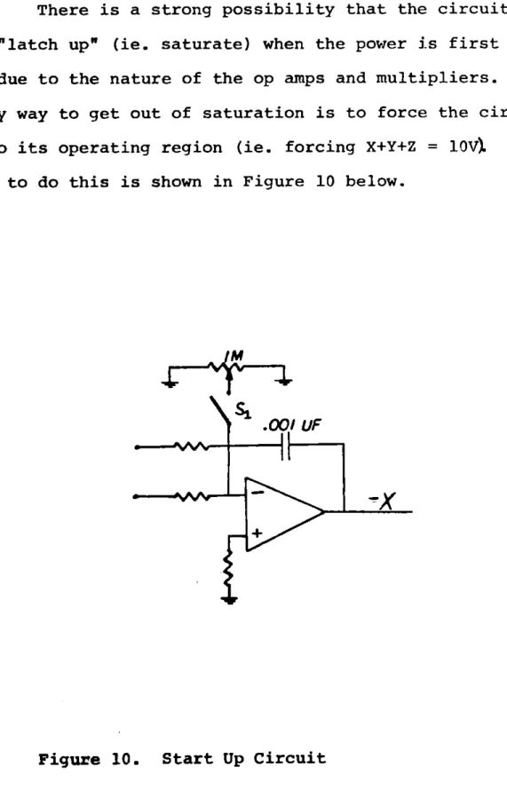
There is a strong possibility that the circuit will "latch up" (ie. saturate) when the power is first turned on due to the nature of the op amps and multipliers. The only way to get out of saturation is to force the circuit into its operating region (ie. forcing X+Y+Z = 10V). One way to do this is shown in Figure 10 below.

.I mU

SX

If switch S₁ is closed, and Z is observed on a voltmeter, appropriate adjustment of the pot will cause Z to change from a saturated voltage to +3V. If S₁ is opened at this time the circuit should oscillate. If not, check over the 13 steps and pay careful attention to the sign of each signal.

Once the circuit is built and oscillating, parameters may be varied to determine the effect on stability. A helpful

addition to the circuit is an audio amplifier and speaker which indicates when the system breaks into limit cycles

and also gives information about the amplitude of the oscillation. The audio circuit which accompanies the SIMKIT is shown below in Figure 11.

The SIMKIT also features buffered signals A, B, X, Y, Z to permit measurement of these variables with low

Audio Circuit. +Vcc 4.711

cc

B. Digital Circu

Having constructed a working analog simulation of the particular system in question, it is desirable to be able to use the circuit to its fullest capability, ie. one would like to know how each variable is behaving and what effect the changing parameter values have on each variable. The use of a remote control channel to

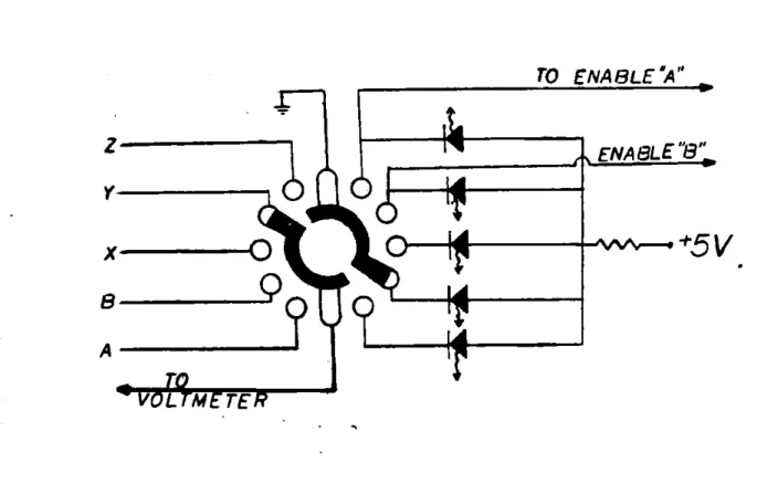
multiplex a DVM or scope to 5 different nodes, serially, affords the user his type of knowledge or insight into the system behavior.

The multiplexing is done via a sonar controlled

stepping motor which advances a six-position switch through positions 1 to 6 representing OFF, A, B, X, Y, and Z

respectively (See Figure 12). One of five indicating LED's is lit to signify which node voltage is being displayed; no LED's lit signify the off position.

The remote control circuit is a tuned circuit which has sharp bandpasses at 35 khz and 40 khz. The sonar

signals are generated mechanically by exciting two bars

(like tuning forks) of different lengths. The 35 kHZ signal activates a relay which advances the stepping motor one

position; while the 40 khz signal advances a four pole single throw switch (Figure 13) by means of a coil magnet and ratchet system.

The stepping motor does the multiplexing by

advancing the switch shown below in Figure 12 one position each time. TO ENABLE "A"

x

o

ot5V.

This switch can be turned either manually or by remote control; but in all cases, the illuminated led indicates the displayed node voltage.

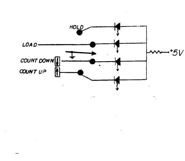
The second channel of remote control is used to

change parameters A and B. The 4 pole switch is capable of rendering 4 logic singnals which control a digital

circuit which adjusts parameters A and B. A schematic of the digital circuit is shown in Figure 14. Note that all four inputs to the circuit are asserted low (ie. a logic zero input asserts control of the circuit).

The Enable input for A is connected to the A terminal of the multiplexing switch. This insures that

the "A" circut will only be enabled when A is being displayed on the DVM. When the multiplexing switch is at this point, it provides the circuit with a logic zero and thus enables the other three control. signals to effect the circuit.

At this point, the second channel of the remote

control comes into play. The four pole switch can provide a logic 0 to any one or none of the remaining 3 input

control lines (ie. LOAD, COUNT UP, OR COUNT DOWN) as

shown in Figure 13. The first position has no effect on the circuit and the value of A remains constant; this is

control which will set A at a specific value which is determined by the wiring of the load inputs of the fp down counters. LOA HOL D n w a IA r 17 COUN T DOWN XVNT UP

Figure 13. 4 Pole Switch Controlling Action of Digital CKT.

(COUNT cow IOOUF 6.2 K IN (COUNT Up) '-9-12X -%, * q -AVL~l .2K (LOAD) 5c0n CENALfE

IL

T

cc

The third position asserts the count up control which starts the 8 bit counter counting digitally upward. The output of the 8 bit counter is brought to a D/A which converts the 8 bit binary signal to an analog voltage A.

The fourth position simply reverses the direction of the counter; while returning to position 1 holds A at its present value. Thus, the second channel of remote control enables the user to set the value of A anywhere between .5V and 1OV. The same circuit is used for

adjusting B ; and thus, the user can adjust A and B

by remote control and observe the effects on stability via

the audio circuit or visually using a scope.

Two important technical difficulties arose in the building of this circuit. The first deals with the

transients associated with the stepping motor. The motor is switched on to advance the multiplexing switch

one position and then the circuit is opened up to stop the motor. Consequently, the magnetic field generated by the motor field-windings suddenly collapses, much like an

ignition coil in a car when the points open up. This rapidly changing magnetic field induces currents in conductors which it crosses perpendicular to the field

lines. These currents were enough to saturate the integrating capacitors and, thus, cause the entire circuit to saturate.

There are many ways to deal with this problem. One way is to use "P metal" to shield the motor; this would be expensive and take too much time. A second way is to alter the direction of the magnetic field by adjusting the field windings as shown in Figure 15 below.

Figure 15. Changing of Motor Windings to Reduce Stray Magnetic Field.

ttfit

A third method of attacking the problem is to use

a sensing circuit which will not turn of f the motor until the current through the windings is zero. The device is an AC motor which precludes the use of a capacitor to mitigate the transient; but enables one to use an SCR circuit to turn off the motor at a zero crossing of current (see Figure 16).

SVAC _MO

Is S2 is now used as the controlling switch, the motor will run after S2 is opened until iL goes to zero

in which case both SCR's become open circuits. I believe that this is the best approach; however, lack of time prompted a fourth approach; that is, to make use of the fact that the magnetic field drops off as an inverse cube law and that the amount of current induced in the circuit is a strong function of the orientation of the magnetic field. Thus, the control box was separated from the computing box and a multiconductor transmission line is used to communicate between the two.

The second technical difficulty encountered was associated with the "bouncing" characteristics of a mechanical switch. In an attempt to provide a logic

zero with a mechanical switch, one encounters oscillations due to the fact that as the switch is closed the contacts bounce off each other for about 50 msecs (see Figure 17 below).

+SV-S3

TonF

SO0

Msecs

i

Figure 17. Bouncing Characteristics of Mechanical Switch. This bouncing problem causes the counters to count the

number of bounces rather than the number of clock pulses which is the desired function. The standard method of

solving this problem is to use an SR flip flop with a double pole single throw switch; however, the switches in the remote control circuit are only single pole single throw switches. Therefore, the only remaining solution

is to use an RC circuit (Figure 18) with a time constant cnparable to the settling time of the switch and which results in a final dc value of v₀ < .8V in order to invert the Schmitt trigger (Figure 19).

5v

V

0

5'V

.8V-. .1450 SECS

The Schmitt trigger is used to interface the slowly

- changing, crude, logic zero with the high speed digital circuit. The transfer characteristics of the Schmitt trigger exhibit hysteresis which reduces the possibility of oscillatior: (see Figure 19).

.16

EF

V

I

.Sv

-I.

v

0

Figure 19. Schmitt Trigger Characteristics Showing Hysteresis Loop.

This method of debouncing a mechanical switch is not as good as the method using a double pole switch with an S-R flip flop mainly because it is a lot slower - about 50-150 msecs slower. However, in this circuit 200 msecs is fast enough, and therefore it is more convenient

and no less desirable to use the RC circuit rather than trying to alter the switches in the remote control box to make them double pole switches.

The SIMKIT, as stated before, has the capability to provide control over parameters A and B. It is also desirable to be able to adjust parameters a , b, and c. Although these controls have not been built, they could be added with similar digital circuits. An important difference between these parameters and A and B are that they multiply variables rather that being summed with them. Control of these parameters can be accomplished by the same circuit as that shown in

Figure 14 with the following alteration. The 8 bits from the up down counter should be connected to 8 switches

(FETS) in a R-2R Ladder (Figure 20) rather than being

x

-1

R

Figure 20. Method of Generating aX Using R-2R Ladder and FET Switches.

The FET switches are closed for a logic zero and open for a logic one; and thus, aX can be varied from X

1

for 8 logic zeroes to 256 X for the LSB logic zero. The other alternative is to use the exact same circuit as Figure 14 and use a multiplier to multiply the analog output with X ; however, this is more expensive and has drawbacks due to the fact that the multipliers aren't as accurate when multiplying voltages less than 1 Volt which "a" is likely to be in this particular system model.

A further suggestion to future designers is to use a different type of remote control circuit. There are

many types of solid state controls which are much less likely to introduce noise into the circuit. The crude stepping

motor and relay switches are much too noisy (both in terms of magnetic and electrical noise as well as audio) and should be left in the past from whence they came.

IV. HOW TO USE THE SIMKIT

The system model being simulated is a rudimentary

element cycle model which is defined by the three equations shown below.

i = aX (-) - bY (-) (1)

X

Y = bY(-) - cY (2)

Z = M - (X+Y) (3)

It has been shown that for a certain range of parameter values, the system exhibits limit cycles. The main purpose of the SIMKIT, as it is now set up, is

to explore the stability boundaries associated with this given ecodynamic system.

To start the circuit, one must first turn on the #15V and +5V supplies and get the circuit out of

saturation. First, display the variable Z on a DVM;

it will be saturated high. Then place the start up switch in the set position (See Figure 21) and adjust the starting pot until Z equals +3.0 Volts. Then switch to Run mode. The circuit should now be in its operating region ie.

X+Y+Z = 10v.

The system at this point is ready to be explored. The parameters a , b , c , and M are set with ten turn

AUDIO CIwCui'r ANALOG CIRCUIT

OIGITAL

CIRCUIT

Figure 21. Overall View of Complete SIMKIT

OA

_-

IMD

0

0

o

cOAO

pots on the terminal board (See Figure 21). They are set at a = .4 , b= .2 , c = .1 , M = 10V , and can be

changed with a small screw driver. A and B are controlled by remote control.

A voltmeter should be plugged into the jack on the

side of the control box; a scope, if available, is also useful. The user should at thi:3 point address B by

first using channel 2 on the transmitter to set the parameter control in the hold position. Then using channel 1, address parameter B. If the system is oscillating it will be

apparent from the audio circuit or the waveforms on the scope. If it is not then proceed to set the parameter control in count down (+) mode. B will continuously fall

in value until the system breaks into oscillations. At this point, the user should set the parameter control to count up (t) and let B increase until the ringing just stops (ie. the system is in equilibrium with no

oscillations). This is a critical point; use channel 1 to address X , Y , + Z respectively, and record each value. This furnishes one point on the stability boundary. In order to obtain more points address N and change its value; then repeat the above procedure. Do this for as many values of A as desired to obtain a corresponding number of critical stability points.

Some sample data is shown below for 7 different values of A (Table I).

TABLE I. Same Data from Stability Experiment

A B 1 2 3 4 5 6 7 2.49 2.61 2.69 2.74 2.81 2.86 2.98 C Xc 2.28 2.37 2.43 2.46 2.51 2.54 2.64 C c 6.10 5.44 4.99 4.64 4.36 4.14 3.97 C Zc 1.64 2.21 2.61 2.92 3.16 3.36 3.43 M 10.02 10.02 10.93 10.02 10.03 10.04 10.04

These points can be plotted to form the stability boundary. Figure 22 shows such a plot in the X-Y

parameter space. The critical points virtually all lie on a straight line which separates the parameter space into stable and unstable regions.

This can be done in any of the three parameter spaces to determine the equation of the straight line stability boundary.

a =.4

b=.2

C

=;

/0/

YW=i7X22

:ST ABL( T Y

BOUNDARY

UNTABL E

ST

ABL E

Figure 22. Experimentally Determined Stability Boundary in X-Y Parameter Space

After determining the stability boundaries for a

given set of parameters a , b , and c, it may be instructive to change one of these parameters and determine the new stability boundaries.

If it is desired to know the exact rate laws which are being represented by the circuit, it is possible to run experiments which accurately determine the actual parameters

associated with these rate laws. Note that the actual parameters a , b , c , A , and B are very close to what

is read on a voltmeter, i.e., if the user sets A at 4.2, he can expect the actual A to be within + 5% of that.

An example can be made of the rate law in equation 1,namely, bY (2w). If the X and Y generators (ie.

X+B

the two integrators) are disconnected and X and Y are generated with pots, one can hold Y constant and vary X and record the value of by( ) for each different value of X. A plotting method called a

Lineweaver-Burke plot enables the user to interpret the data to yield the precise values of b and B.

Consider R = bY( &B) to be the equation in question. If one takes the reciprocal of both sides of the equation,

= 1 B 1 . .

he gets 1=() + (- )g which is the equation of a

1 1

straight line relating .1to 1. Using the data points XI R

these points. The straight line will give information

1 B

about the intercept, - and the slope . Since Y

was held constant, the parameters b and B can be determined.

A sample experiment was done with Y set to 3.OV

b = .2 , and B = 2.5V. The sample data is given in TABLE II and plotted in Figure 23. As can be seen from

the graph, the points do come very close to falling in a straight line. This line has a slope of 4.6 and an inter-cept of 1.8 which imply that b = .19 and B = 2.6. Thus, the actual values are, indeed, close to the values

which were set using the voltmeter.

TABLE II.

x

Sample Data for Linewaver-Burke Plot

1 1 1.54 8.33 .97 5.88 .65 4.55 .51 4.08 .35. 3.23 .22 2.77 .15 2.44

.

8+

4.6

0

4.6

=

=2.d6

=1

=.9

.5

4

-r

b=.2

8=2.5

Y=3

I

5

I

/.0

x

This method can also be used to determine accurately

Z

the other rate law aX( Z+A) , and the user is invited to apply the Lineweaver-Burke method to further convince himself of the accuracy of the rate laws.

V. CONCLUSION

The Sim-Kit idea proposed by Professor Paynter to model an ecodynamic system model formed by

Alician Quinlan and himself has proven to be feasible.

During the course of this project there were some technical problems, however, none of them too great to render it

impractical. The major suggestion for alteration of the present kit is the acquistion of a solid state

remote control circuit to provide clear (ie. noiseless) switching and perhaps more channels to exert greater control over the circuit.

The main use of the Sim-Kit is as an interactive teaching aid; it enables the user to "feel", see, and hear the system behave as it suddenly breaks into limit cycles and falls back into equilibrium. The concept of stability boundaries derived by mathematical manipulation of system equations becomes a tangible and meaningful thing as one alters parameter values and traverses stable and unstable regions. The student acquires an invaluable intuitive "feel" for the system which can rarely be found through inspection of system equations.

Thus, it is clear that the SIMKIT idea is both a feasible and valuable one that warrants further development.