The MIT Faculty has made this article openly available. Please share
how this access benefits you. Your story matters.
Citation Mohammadi Ghazi, Reza, and Büyüköztürk, Oral. “Damage Detection with Small Data Set Using Energy-Based Nonlinear Features.” Structural Control and Health Monitoring 23, 2 (July 2015): 333–348 © 2015 John Wiley & Sons
As Published http://dx.doi.org/10.1002/stc.1774
Publisher Wiley Blackwell
Version Original manuscript
Citable link http://hdl.handle.net/1721.1/112156
Terms of Use Creative Commons Attribution-Noncommercial-Share Alike
For Peer Review
Damage detection with small data set using energy-based nonlinear features
Journal: Structural Control and Health Monitoring Manuscript ID: STC-14-0201.R1
Wiley - Manuscript type: Research Paper Date Submitted by the Author: n/a
Complete List of Authors: Mohammadi Ghazi, Reza; Massachusetts Institute of Technology, Civil and Environmental Engineering
Büyüköztürk, Oral; Massachusetts Institute of Technology, Civil Engineering
Keywords:
Energy method, hypothesis testing, Marginal Hilbert spectrum, Mahalanobis distance, white noise excitation, normalized cumulative energy distribution, nonlinearity
For Peer Review
Damage detection with small data set using energy-based nonlinear
features
Reza Mohammadi Ghazi1 and Oral Büyüköztürk2
Department of Civil and Environmental Engineering, Massachusetts Institute of Technology, 77 Massachusetts Avenue, Cambridge, MA 02139, USA
Abstract
This study proposes a new algorithm for damage detection in structures. The algorithm employs an energy-based method to capture linear and nonlinear effects of damage on structural response. For more accurate detection the proposed algorithm combines multiple damage sensitive features through a distance-based method by using Mahalanobis distance. Hypothesis testing is employed as the statistical data analysis technique for uncertainty quantification associated with damage detection. Both the distance-based and the data analysis methods have been chosen to deal with small size data sets. Finally, the efficacy and robustness of the algorithm is experimentally validated by testing a steel laboratory prototype and the results show that the proposed method can effectively detect and localize the defects.
Keywords
Energy method, hypothesis testing, marginal Hilbert spectrum, normalized cumulative energy distribution, Mahalanobis distance, white noise excitation
1
Doctoral Candidate, Department of Civil and Environmental Engineering, Massachusetts Institute of Technology, Massachusetts, USA. Email: [email protected]
2
Corresponding author:
Professor, Department of Civil and Environmental Engineering, Massachusetts Institute of Technology, Massachusetts, USA. Email: [email protected]
3 4 5 6 7 8 9 10 11 12 13 14 15 16 17 18 19 20 21 22 23 24 25 26 27 28 29 30 31 32 33 34 35 36 37 38 39 40 41 42 43 44 45 46 47 48 49 50 51 52 53 54 55 56
For Peer Review
Introduction
Vibration based structural health monitoring (SHM) is a widely used method for monitoring large scale, complex structures. Aging of infrastructures, higher operational demands, and variety of environmental effects on structural systems are the main reasons that attract more attention to this field in recent years.
The algorithms for vibration-based SHM are either model-based or data-based. Both methods compare the response of the system with a baseline. In model-based approach, the baseline is provided using numerical models. Thus, this method is helpful for systems for which the model already exists and in cases where it is justifiable to build a sufficiently accurate structural model [1-3]. The data-based approach brings more flexibility to the damage detection scheme since it only uses the sensor data without having to deal with the complications of creating a model. The initial phase in both of these methodologies is feature extraction. In this phase certain damage sensitive features, called damage index (DI), are extracted from the structure’s response, either empirically obtained or numerically simulated, to measure its discrepancies from the response in the intact state. Previous studies show that the features which capture nonlinearities in the structural response are generally more sensitive to damage, less sensitive to environmental conditions, and hence, more reliable for the purpose of damage detection compared to the DIs that capture linear phenomena such as modal properties [4-7]. Note that the source of nonlinearities can be material, geometry, or nonlinear dynamics phenomenon such as dispersion, mode mixing, and damping. The fractal dimension of the attractor of time-series is the basis for defining DIs in [8-11]. Fractal analysis of residual crack patterns in reinforced concrete structures [12], state-space reconstruction using the delay-coordinate method [13,14], considering systems under chaotic excitations [15], sensitivity vector
3 4 5 6 7 8 9 10 11 12 13 14 15 16 17 18 19 20 21 22 23 24 25 26 27 28 29 30 31 32 33 34 35 36 37 38 39 40 41 42 43 44 45 46 47 48 49 50 51 52 53 54 55
For Peer Review
field [16,17], Poincare’ map based methods [18-22], and nonlinear frequency response function [23-26] are examples of techniques that use nonlinearities in monitoring structures. The variety and efficacy of these methods show that nonlinearities hold a great potential for damage detection.
Generally, extracting nonlinearities requires expensive computational effort. Moreover, some necessary conditions for the nonlinear algorithms may not be easily satisfied in practice. For instance, the technique in the sensitivity vector field [16] focuses on deviation of nearby trajectories corresponding to the intact and damaged system. The method uses the variation between those trajectories instead of linearization, and hence retains nonlinearities. However, the algorithm is sensitive to the closeness of the trajectories which cannot be always satisfied in practice. As another example, the concept of nonlinear frequency response function (NFRF) which is discussed in [23-25] and used for crack detection in [26] may not preserve all nonlinearities in the signal. The reason is that Fourier-based methods may suffer from leakage of energy due to imposition of spurious harmonics on the expansion of a signal.
Given that we have reliable and practical DIs, there are two other requirements for practicality of the algorithms: 1) taking an appropriate decision-making approach to interpret the final results, 2) generalization of the method. A statistical decision making approach, instead of classifying the structure solely based on the DI values, is needed for practicality of a damage detection algorithm. Some studies have proposed methods for uncertainty quantification in SHM [27], but few of them have been experimentally validated. Additionally, the effect of damage may not be always reflected in all DIs; therefore, using multiple DIs would increase the probability of detection and helps in the generalization of the method. However, appropriate data analysis and decision-making procedures should also be adapted.
3 4 5 6 7 8 9 10 11 12 13 14 15 16 17 18 19 20 21 22 23 24 25 26 27 28 29 30 31 32 33 34 35 36 37 38 39 40 41 42 43 44 45 46 47 48 49 50 51 52 53 54 55 56
For Peer Review
This study proposes a damage detection/localization algorithm with three main objectives: 1) developing a simple and practical method for capturing nonlinearities, 2) Combining DIs in order to increase the accuracy and reliability of the algorithm, 3) adopting a statistical decision-making approach, especially for dealing with small size data sets.
For defining the DIs, we propose an energy-based algorithm which captures linear and nonlinear effects of damage. Hilbert Huang Transformation (HHT) is adopted as the signal processing tool for the algorithm because of its ability for preserving nonlinearities and preventing the leakage of energy [28]. We have chosen hypothesis testing as the probabilistic decision making approach due to its computational efficiency and ability to deal with small size data sets. Finally, the developed algorithm and its efficacy are validated by testing a three-story two-bay steel laboratory prototype with several damage scenarios.
Energy transfer between modes of vibration due to damage
Structural damages such as breathing cracks, loosened bolts in a connection, yielded cross-section, and corrosion result in geometric and/or material discontinuities in a system. Such discontinuities affect the system’s response by either changing the frequency content of existing vibrational modes or bringing new degrees of freedom (DOF) and hence, new modes of vibration. In either case, the energy content of vibrational modes are changed by exchanging energy between existing modes or transferring energy from existing modes into newly generated ones. These phenomena are manifested in the energy distributions between vibrational modes of the system, such as Power Spectral Density (PSD), as the shift and/or suppression/amplification of some peaks. Therefore, the pattern of the energy distribution between vibrational modes of a
3 4 5 6 7 8 9 10 11 12 13 14 15 16 17 18 19 20 21 22 23 24 25 26 27 28 29 30 31 32 33 34 35 36 37 38 39 40 41 42 43 44 45 46 47 48 49 50 51 52 53 54 55
For Peer Review
system can be considered as a signature to be used for capturing the variations in both the linear and nonlinear properties of the structure.
The proposed algorithm in this study has a fundamental assumption that the excitations on the structure are consistent. This means that the differences between the input energies or spectrums of different excitations cause neither damage occurrence nor any significant change in the modal behavior of the structure. This assumption is generally a constraint for vibration-based SHM algorithms, especially when the forced response of the system is used as the input.
Normalized Cumulative Marginal Hilbert Spectrum (NCMHS) and
Normalized Cumulative Power Spectral Density (NCPSD)
In this section, we discuss how to obtain an appropriate distribution of energy for capturing nonlinearities. Some candidates for the energy distribution between vibrational modes are the Power Spectral Density (PSD), wavelet spectrum, and Marginal Hilbert Spectrum (MHS). For reliability and accuracy of the algorithm, a distribution with the least possible energy leakage of any form is needed. This criterion implies that PSD may not be a good candidate since it suffers from the leakage of energy due to imposition of spurious harmonics on the expansion of a signal. Wavelet is also a linear signal processing technique that suffers from the same problem as PSD does [28] although it has no assumption of stationarity. MHS seems to be more reliable than the other two distributions as it preserves the nonlinearities without imposing any spurious modes on the expansion of a signal. Moreover, the definition of frequency which is used in HHT is conceptually more appropriate for the sake of damage detection. For different definitions of frequency and concept of each, the readers are referred to [29]. Also, a comprehensive discussion
3 4 5 6 7 8 9 10 11 12 13 14 15 16 17 18 19 20 21 22 23 24 25 26 27 28 29 30 31 32 33 34 35 36 37 38 39 40 41 42 43 44 45 46 47 48 49 50 51 52 53 54 55 56
For Peer Review
on the inconsistencies of the concept of frequency in Fourier domain for nonlinear signal processing can be found in [28].
These energy distributions are non-smooth and mathematically difficult to deal with. Note that the sensor data are discrete and continuity or smoothness for such functions may not be meaningful. In this paper, a smooth distribution refers to the one with invariant sign of derivative. Also, note that smoothening the curves by approximate continuous functions is not an appropriate solution because the true physics such as the effects of high frequency modes, which are important from SHM point of view, may be totally lost. Instead of smoothening, in this study, we propose to use the cumulative energy distribution with the advantage that it monotonically increases and that there is no loss of physics or leakage of energy. If the assumption of consistent excitations holds, the energy distributions can also be normalized with respect to their total energy with no lack of generality. The resultant distribution in this case is called Normalized Cumulative Marginal Hilbert Spectrum (NCMHS) if MHS is the original energy distribution. In the case of PSD, the resultant curves are called Normalized Cumulative PSD (NCPSD). The normalization is not valid if the excitations are inconsistent.
Damage Indices
In view of the preceding discussion, we propose the use of normalized cumulative energy distribution (NCED) as a reliable signature for a system under consistent excitations. In what follows we discuss how to obtain a baseline NCED for the structure’s response at each sensor location and then, how to define the DIs for measuring the NCED’s damage-induced discrepancies from the baseline.
3 4 5 6 7 8 9 10 11 12 13 14 15 16 17 18 19 20 21 22 23 24 25 26 27 28 29 30 31 32 33 34 35 36 37 38 39 40 41 42 43 44 45 46 47 48 49 50 51 52 53 54 55
For Peer Review
DIs from normalized cumulative energy distributions
Using the NCED, the first DI is defined as
BL i i A A
∑
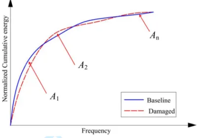
= 1 DI (1)where Ai, as shown in Fig. 1 are the areas between the NCED of the structure being monitored
and the baseline. ABL is the area under the baseline NCED which is computed by taking the mean
or median of such distributions from several tests on the intact same structure. Taking median, as we do in this paper, is preferable because of its robustness with respect to outliers, especially for small sample size.
Normalization of the energy distribution allows us to compare NCEDs by the similar techniques for comparing probability distributions. For instance, Kolmogorov-Smirnov distance is one such a method that we use for DI2 in eq. (2).
) , (
DI2 =Dn FT FBL (2)
where Dn is the Kolmogorov-Smirnov statistic and n is the sample size. FT and FBL are the
NCEDs for the test data and the baseline, respectively.
Note that DI2 captures a local effect of energy transfer which may be highly sensitive in certain cases. Thus, DI3 is proposed as a more general index for capturing the overall changes in the pattern of distributions using the concept of orthogonality.
BL T BL T F F F F . DI3 = ⋅ (3)
The numerator is the inner product of the NCED of new test with the baseline, and the denominator is the multiplication of their norms. This index could also be defined for the original
3 4 5 6 7 8 9 10 11 12 13 14 15 16 17 18 19 20 21 22 23 24 25 26 27 28 29 30 31 32 33 34 35 36 37 38 39 40 41 42 43 44 45 46 47 48 49 50 51 52 53 54 55 56
For Peer Review
energy distributions, but it would be more sensitive to noise. Any other measure of local or global discrepancy between the NCED and the baseline can be used as a DI.
DIs from the original energy distributions
There exist certain indices which are physically interpretable only if they are extracted from the original distribution, MHS or PSD. As before, one can normalize the original distributions based on the assumption of excitation consistency with no lack of generality. The shift of the mean frequency in the response at each sensor location of the test structure from its baseline is one such index that can be defined using the original distribution. This DI is
BL BL T f f f − = 4 DI (4)
where f and T f are the mean frequencies in the spectrum of the test data and the baseline, BL respectively. The denominator makes the DI dimensionless. Alternatively, max(fBL), where f is
the frequency range of spectrum, can be used in the denominator to keep this index between zero and unity.
Skewness is another property which shows the direction of energy accumulation with respect to mean frequency. Kurtosis can also be used as a measure of peakedness of the distributions which was used in [30] as the only DI. The sign of the argument of the absolute value function in the numerator of DI1 and DI4 can also be used for a rough severity assessment [31]. 3 4 5 6 7 8 9 10 11 12 13 14 15 16 17 18 19 20 21 22 23 24 25 26 27 28 29 30 31 32 33 34 35 36 37 38 39 40 41 42 43 44 45 46 47 48 49 50 51 52 53 54 55
For Peer Review
Combining damage indices and uncertainty quantification
Damage may not always be manifested in every single DI. Also, it may not be realistic to make decision about the state of the structure based only on the value of a specific index. Our approach for solving this issue is to combine several DIs for a better detection/localization and to quantify the confidence associated with detection. Note that in statistical learning theory and machine learning some scores may be normalized and calibrated using a set of calibration data, and reported instead of true probabilities. This method cannot be pursued here since the problem is unsupervised.
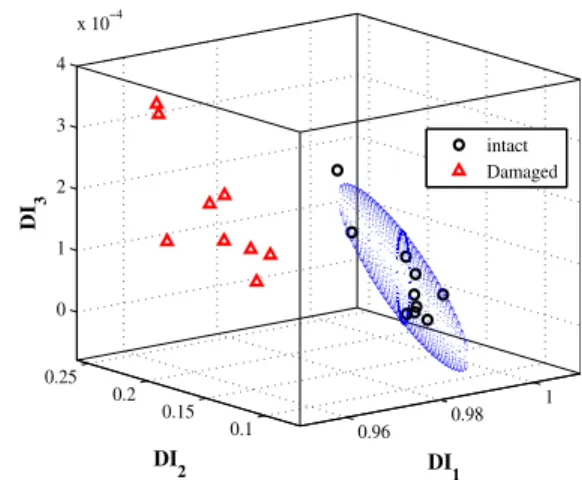
By conducting an experiment on a structure, its behavior at each sensor location can be described by an m-dimensional feature vector, with m to be the number of DIs being considered simultaneously. By performing several experiments on the intact structure and extracting the DIs from the data, a cluster of feature vectors is formed. This cluster, which is called the intact cluster, represents the expected deviations from the baseline when the system is intact. Similarly, a second cluster can be formed by taking measurements from the structure in an unknown state when being monitored. This cluster is called test cluster and shows the actual deviation from the baseline. Fig. 2 shows the intact and test clusters in three-dimensional feature space. Assuming multivariate normal (MVN) distribution for the points in each cluster due to the repeatability of the tests, hypothesis testing is used in this study for comparing the two clusters at each sensor location.
Generally, the size of data set may be small in structural health monitoring, especially for large scale structures or at the beginning of instrumentation. Hypothesis testing is used as the data analysis technique in this study because of its capability of making inference on small size data sets with lower cost and error compared to other big data classification methods [32]. Note
3 4 5 6 7 8 9 10 11 12 13 14 15 16 17 18 19 20 21 22 23 24 25 26 27 28 29 30 31 32 33 34 35 36 37 38 39 40 41 42 43 44 45 46 47 48 49 50 51 52 53 54 55 56
For Peer Review
that in practice, the collinearity and correlation between different DIs significantly affect the robustness of the algorithm [33]. For more information on how to optimally shrink the dimension of feature space the readers are referred to [34].
Performing hypothesis testing in the m-dimensional feature space can be considered for comparing two general clusters of feature vectors. However, inaccurate results may be obtained from such a test when the features are all positive or fall in certain quadrants only. In this case the m-dimensional test computes unrealistically high p-values, which are the probability of accepting a null hypothesis that represents the intact state of the system. To clarify this, assume nI and nT are the number of points of the intact and test clusters, respectively. They are, in fact,
the number of experiments performed on each of the respective structures. The mean value of each cluster is denoted, respectively, by mI and m . Then, the null hypothesis for comparing T
the clusters’ mean values is
T I
H0:m =m (5)
The test statistics is defined as the difference between the mean values as in eq. (6)
I T m
m
m= −
∆ (6)
Then, the null distribution would be a zero mean MVN distribution stated in eq. (7)
(
)
+ ∆ T T I I n n N H O Σ Σ m| 0 ~ , (7)where ΣI and Σ are the covariance matrices of the intact and test clusters, respectively. For T
simplicity, the covariance of the null distribution is denoted by Σ . The set of points denoted by x
in the hyper-space that satisfy eq. (8) form a hyper-ellipsoid of the mentioned density function which passes from m . T
3 4 5 6 7 8 9 10 11 12 13 14 15 16 17 18 19 20 21 22 23 24 25 26 27 28 29 30 31 32 33 34 35 36 37 38 39 40 41 42 43 44 45 46 47 48 49 50 51 52 53 54 55
For Peer Review
2 1
:xTΣ− x=β
E (8)
where the superscript T is the transpose. β is the Mahalanobis distance between the mean values of the clusters conditioning on the null hypothesis:
m Σ m ∆ ∆ = −1 2 T β (9)
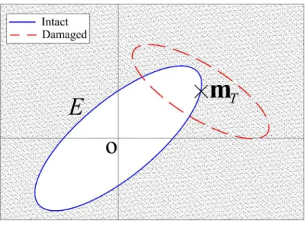
The p-value is calculated by computing the hyper-volume outside of the hyper-ellipsoid E defined in eq. (8). This is shown as the shaded zone in Fig. 3 for 2D case. As it was stated before, the DIs are always positive by definition; thus, the m-dimensional hypothesis testing gives a much higher p-value since it calculates spurious probabilities due to consideration of the whole space. With general covariance matrix, calculating the probability only at the first quadrant may not be tractable. Neither mapping the null distribution to a spherical MVN nor using the whitening transformation [32] change the complexity of the problem; because, either the axis of the space do not remain orthogonal or the feature vectors may not stay in the first quadrant.
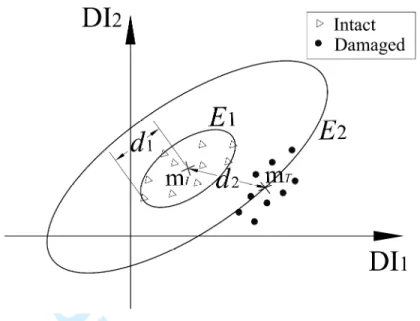
Instead of performing the m-dimensional test, we use Mahalanobis distance [32,33] to map the m-dimensional feature space into a dimensional distance space and then, perform one-dimensionl hypothesis testing. Due to the consideration of the covariance matrix, Mahalanobis distance is more robust compared to other distances for comparing clusters. Fig. 4 illustrates an example in which Euclidian distance fails to capture the discrepancy of the two clusters when DI1 is insensitive to the damage. In this plot, E1 is the ellipse corresponding to the farthest point of the intact cluster to its mean value and d1 is the Euclidian distance between these two points. E2 is the ellipse corresponding to the Mahalanobis distance between the mean values of two clusters conditioning on the null hypothesis, and d2 is the Euclidian distance between them. It
3 4 5 6 7 8 9 10 11 12 13 14 15 16 17 18 19 20 21 22 23 24 25 26 27 28 29 30 31 32 33 34 35 36 37 38 39 40 41 42 43 44 45 46 47 48 49 50 51 52 53 54 55 56
For Peer Review
follows from Fig. 4 that the Euclidian distances, d1 and d2, cannot capture the difference between the two clusters; whereas, such a difference is clearly reflected in the Mahalanobis distance.
In the following four steps we describe the algorithm for detecting and localizing the damage by taking the data sets from each sensor and analyzing them.
Step1: Calculate
( )
βI2 i, the squared Mahalanobis distance of the ith point of the intact cluster from the rest of the points of the same cluster using eq. (10)( )
(
( )
) ( )
(
( )
i)
I i I i I T i I i I i I − − − − − − = x m Σ 1 x m 2 β (10)where
( )
xI i is the ith point in the m-dimensional space belonging to the intact cluster and{
nI}
i= 1... . m and I−i Σ are the mean and covariance estimates of the intact cluster I−i
without the ith point.
Step2: Calculate
( )
βT2 j, the squared Mahalanobis distance of each point of the cluster for the test structure from the whole intact cluster. The mentioned distance is computed as( )
(
( )
)
( )
I(
( )
T j I)
T I j T j T = x −m Σ x −m −1 2 β (11)where
( )
xT j is the jth feature vector, j={
1...nT}
, in the m-dimensional space belonging to the cluster for the test structure. m and I Σ are, respectively, the mean and covariance of Ithe full intact cluster.
Step3: Perform a one-sided, one-dimensional hypothesis testing on
{
( )
( )
}
I n I I I 2 1 2 2 , , β β K = β and( )
( )
{
T T nT}
T 2 1 2 2 , , β β K =β . If both clusters are normally distributed, both β and I β follow T
the Chi-squared distribution with m degrees of freedom. Another alternative to that, is to perform a one-sided, one-dimensional hypothesis testing using
{
( )
( )
}
I n I I I = β 1,K, β β 3 4 5 6 7 8 9 10 11 12 13 14 15 16 17 18 19 20 21 22 23 24 25 26 27 28 29 30 31 32 33 34 35 36 37 38 39 40 41 42 43 44 45 46 47 48 49 50 51 52 53 54 55
For Peer Review
and{
( )
( )
}
T n T T T = β 1,K, ββ with the assumption of normality for both β and I β if the T
sample size is reasonably large for this assumption [32]. The null hypothesis here is that the mean values of the β and I β are equal. T
Step 4: Once the null hypothesis is rejected at any sensor location, which implies that the structure is damaged, the defect can be localized by a localization index, denoted by Rβ in eq. 12. Med(.) in this equation stands for the median of the argument. The damage is likely to be at or adjacent to the sensor locations with larger Rβ.
) Med( ) Med( ) Med( 2 2 2 I I T R β β β − = β (12)
It is noteworthy that the detection results using the p-values may not be used for localization, especially for small and low damping structures. The reason is that neither the normal nor the chi-squared distributions are heavy tail densities; therefore, if the centroids of the intact and test clusters are more than two standard deviations away in normal distribution, the null hypothesis is rejected with very small p-values. This may happen for several sensor locations, especially if the damage is severe or the structure is small. However, there is no such limitation for the Mahalanobis distance and hence, the ratio Rβ can always be used for damage localization.
The procedure for the proposed algorithm is schematically shown in Fig. 5. Several parameters such as cost of inspection, importance of the structure, and secondary effects of damage on the environment should be considered for determining the significance level of the test denoted by α in that figure. Note that the method can be used for any structure since the algorithm requires only the sensor data with no information about the properties or the geometry
3 4 5 6 7 8 9 10 11 12 13 14 15 16 17 18 19 20 21 22 23 24 25 26 27 28 29 30 31 32 33 34 35 36 37 38 39 40 41 42 43 44 45 46 47 48 49 50 51 52 53 54 55 56
For Peer Review
of the system. Another important aspect of the algorithm is its capability of performing automatically after predefining the significance level.
It is emphasized that the mean value is not robust with respect to outliers. Also, the effects of outliers on the results become more significant as the size of data set becomes smaller. To avoid this problem, one can use median for defining the null hypothesis instead of the mean. In this case, the hypothesis testing is not parametric and eq. (7) is no longer valid. Instead, a non-parametric hypothesis testing such as Mood’s median test can be performed to compute the p-values. Performing such a test affects only the third step of the proposed algorithm. More specifically, the null hypothesis states that the medians of βI and βT are equal. Then the Moon’s test is performed by counting the number of samples smaller/larger than the medians followed by a chi-squared test. Kruskall-Wallis test [33] is another non-parametric method for comparing the two clusters by using the rank of observations in each vector βI and β to perform the test. T The rank in this test is defined as the position of sample points after sorting them with respect to their magnitude. The rank is robust with respect to outliers and hence, they are not significantly influential in this method. Note that there is no assumption of normality in Moon’s and Kruskall-Wallis tests, thus, they can be used when βI and βThave arbitrary distributions [33].
As it was mentioned before, the collinearity of the features may result in inaccurate damage localization. To solve this problem, the Mahalanobis distances can be computed after selecting the most informative subset of the features. Soft-thresholding by considering the first two principal components of the features is employed for dimension reduction in this study.
In some cases, the sensitivity of each DI to the damage may be used for selecting/excluding some features prior to the dimension reduction. To assess the sensitivity of
3 4 5 6 7 8 9 10 11 12 13 14 15 16 17 18 19 20 21 22 23 24 25 26 27 28 29 30 31 32 33 34 35 36 37 38 39 40 41 42 43 44 45 46 47 48 49 50 51 52 53 54 55
For Peer Review
the ith DI at each sensor location first we form the vector yIi by r times sampling with replacement from the ith column of xI. Similarly, the vector yTi is formed by sampling from the ith column ofxT. The sensitivity of the ith DI to the damage can be assessed by considering the statistical moments of the vector EDI−i which is defined as
Ii Ti i DI E − = y −y (13)
Experimental setup
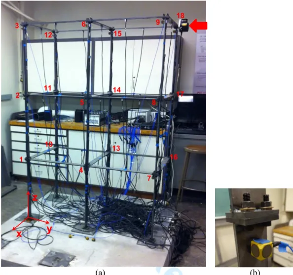
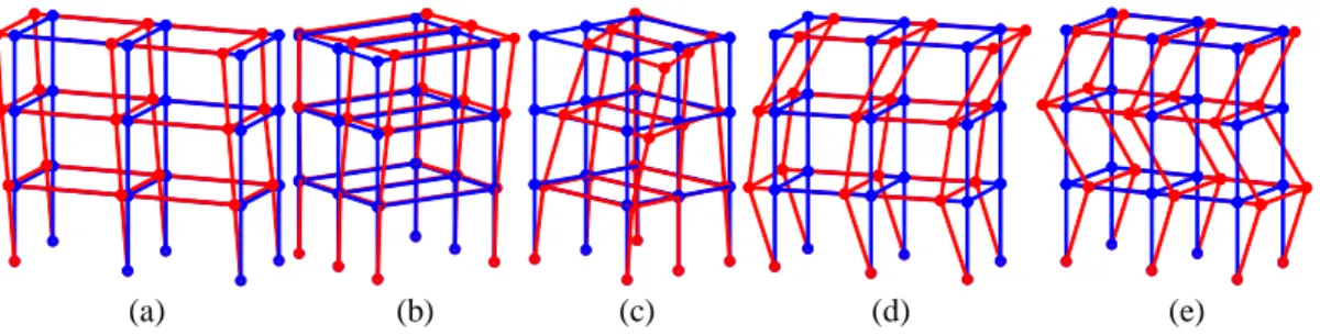
The efficacy of the proposed algorithm have been experimentally validated by testing a three-story two-bay laboratory steel structure which is shown in Fig. 6. The modal properties of the structure are computed using frequency domain decomposition [35] and illustrated in Table 1. The first five mode shapes are also shown in Fig. 7. It should be mentioned that the second mode was a minor peak of the singular values of the PSD matrix. The modal analysis shows that the stiffness of the structure in x direction is significantly larger than y direction. The reason for that is the geometry of the elements.
The structure is instrumented with 18 triaxial piezoelectric accelerometers. The bolts in all connections are completely tightened for the intact structure. By removing or loosening some of the bolts, several damage scenarios can be produced. The scenarios which are used in this paper are summarized in Table 2. For introducing the minor damage, two bolts on one side of a connection are removed while the other two bolts are kept firmly tight. For the major damages all four bolts are tightened using half of the torque needed for a completely fixed connection.
Therefore; the connection is not clamped, but no instability occurs. The structure is tested 10 times for the intact and each of the damage scenarios. The excitation is free vibration for the first
3 4 5 6 7 8 9 10 11 12 13 14 15 16 17 18 19 20 21 22 23 24 25 26 27 28 29 30 31 32 33 34 35 36 37 38 39 40 41 42 43 44 45 46 47 48 49 50 51 52 53 54 55 56
For Peer Review
two scenarios and White Gaussian noise for the third one. For the third scenario, the structure is excited by a shaker mounted at node #18 which is shown by an arrow in Fig. 6. Both excitations are in y direction and the sampling rate of data acquisition is 6 kHz; however, we use frequencies up to 500 Hz for computing the energy distributions to simulate a more practical case.
Results
In this part, first the efficacy of the algorithm to detect and localize damages is experimentally validated followed by checking of a required condition for robustness of the algorithm.
Damage detection and localization
Scenarios under free vibration
Fig. 8 and Fig. 9 show the MHS and NCMHS respectively for nodes #17 and #14, which are adjacent, before and after the occurrence of damage at node #17. The response deviates from the baseline at both nodes after the occurrence of damage; however, as expected, the deviations are larger at node #17 where the damage is located.
The damage detection results for the first two scenarios are shown in Fig. 10. The y-axis of these plots is 1-(p-value), which is the probability of rejecting the null hypothesis. The null hypothesis is rejected at a sensor location if the corresponding p-value is less than α , or equivalently, if 1− p
(
-value)
>(1−α). The two horizontal lines in the figure correspond to two significance levels: for the red line α =0.05 and for the green line α =0.10. In the first scenario with minor damage, the null hypothesis is rejected only at the nodes which are adjacent to the3 4 5 6 7 8 9 10 11 12 13 14 15 16 17 18 19 20 21 22 23 24 25 26 27 28 29 30 31 32 33 34 35 36 37 38 39 40 41 42 43 44 45 46 47 48 49 50 51 52 53 54 55
For Peer Review
the p-values. For the major damage scenario, Fig. 10(b), almost every sensor location is affected
due to the severity of the damage, small size of the laboratory prototype, and its low damping. Therefore, the information provided by the p-values is only appropriate for detecting the damage.
As it is shown in Fig. 10(b), the damage may not be localized precisely by considering only the p-values. In such cases, the localization index, Rβ, is used for damage localization. The localization results for the first two damage scenarios are shown in Fig. 11. In this figure Rβ is plotted on y-axis in logarithmic scale versus the node numbers on x-axis. As shown in this plot,
the localization index is at least one order of magnitude larger at the damage location or proximal nodes than those at other locations. For the minor damage, Fig. 11(a), although node #17 and its adjacent nodes #8, #14, and #16 are separated from the other sensor locations, the localization index is not the highest at the actual damaged location. The reason for that could be the low severity of the damage, small size of the structure, and its low damping. In the major damage scenario, the localization index has the highest value at node #17 and decreases as we go further from the damaged location.
Both Fig. 10 and Fig. 11 also compare the results when PSD and MHS are used as the input to the algorithm. It is observed that the damage cannot be localized precisely if PSD is used as the energy distribution. The authors believe that the artificially high p-values and the
inaccurate localization in the case of using PSD are mainly due to the energy leakage in Fourier transformation.
Note that, as shown in Fig. 12, for major and minor damage scenarios the individual indices DI1 and DI2 have the highest sensitivity and DI4 has the lowest sensitivity to the damage.
Also, both the standard deviation and the median of EDIis higher at the location of damage and
3 4 5 6 7 8 9 10 11 12 13 14 15 16 17 18 19 20 21 22 23 24 25 26 27 28 29 30 31 32 33 34 35 36 37 38 39 40 41 42 43 44 45 46 47 48 49 50 51 52 53 54 55 56
For Peer Review
its adjacent nodes, especially for the major damage. Note that this result cannot be generalized and the sensitivity of the features depends on the structural properties, type, and severity of damage.
The scenario with major damage at node #1 and white noise excitation
In this scenario both the intact and damaged structures are excited under white Gaussian noise in order to analyze the robustness of the algorithm with respect to a higher level uncertainty in excitation consistency. The shaker, which is mounted to the structure at node #18 (Fig. 6(a)), can simulate excitations with frequency band between 5 Hz to 350 Hz. Therefore, all other components with frequencies out of this range impose uncertainties on the excitation consistency.
The detection and localization results for this scenario are shown in Fig. 13. The results with MHS precisely localize the damage. The value of the localization index at node #18 is in the same order of magnitude as in nodes #3 and #10 which are adjacent to the damage. This can be due to mounting the shaker at node #18. The relatively flat trend of Rβ when PSD is used for this scenario, where the broad band excitation results in imposing more spurious harmonics on the Fourier expansion, implies the significance of the energy leakage. The sensitivity assessment of the DIs in this scenario is similar to the previous cases and hence, the corresponding results are excluded for brevity.
Robustness of the algorithm
A necessary, but not sufficient, condition for robustness of the algorithm is that it should not detect any damage after repairing the structure. To address this issue, we repaired the
3 4 5 6 7 8 9 10 11 12 13 14 15 16 17 18 19 20 21 22 23 24 25 26 27 28 29 30 31 32 33 34 35 36 37 38 39 40 41 42 43 44 45 46 47 48 49 50 51 52 53 54 55
For Peer Review
structure and tested it five times with similar excitations as before. Fig. 14 shows the damage detection results of the repaired structure. Note that we perform one-sided hypothesis testing; thus, the p-value of 0.5 corresponds to a perfect match between the mean values of the clusters.
As observed, the algorithm with MHS gives us almost perfect results. The results, however, are more scattered when PSD is employed and the algorithm rejects the null hypothesis at node #9 in this graph.
The algorithm seems to be robust when MHS is used; however, the authors do not disregard the use of PSD because Fourier analysis is computationally more efficient than HHT. Combining some other well-developed algorithms for feature selection can be a solution to compensate for the shortcomings of PSD. This aspect is outside the scope of this paper.
Discussion on size effect
and noise filtration
Size effects, as may be related to the size of the element, the system, and the damage, is an important consideration which may influence the accuracy of the detection results as well as the robustness of an algorithm. For instance, even the mass of a sensor may significantly change the modal properties of a small beam element; while, such a change in mass may be negligible for a full scale beam element. Therefore, the size effect should be taken into consideration, especially for qualitative assessments such as severity of damage.
A final point is about filtering out the noise from the signal. Note that the band-pass filters which use Fourier transformation impose spurious harmonics on the signal and hence, cause energy leakage. To solve this problem, an intermittent frequency can be imposed before the sifting procedure of EMD [36-38]. By doing that, the riding waves with frequencies above the intermittent frequency are first extracted without causing any leakage. Then, the remaining signal
3 4 5 6 7 8 9 10 11 12 13 14 15 16 17 18 19 20 21 22 23 24 25 26 27 28 29 30 31 32 33 34 35 36 37 38 39 40 41 42 43 44 45 46 47 48 49 50 51 52 53 54 55 56
For Peer Review
is sifted through EMD procedure. The intermittent frequency, similar to α , can be set in the initialization step of the algorithm.
Conclusion
In this study a new damage detection algorithm is proposed. Salient aspects of this algorithm are employing an energy-based method for extracting linear and nonlinear effects of damage, and combining several DIs for increasing the probability of detecting damage. Moreover, it quantifies the uncertainties associated with detection when the size of data set is small. The raw signals of structural response are the only input to the algorithm and no information on geometry, configuration, and material of the structure is needed.
Experiments on the laboratory model structure show that damage-induced nonlinearities in the structural response can be effectively captured by the energy-based method. Using the proposed features, the algorithm provides a measure of uncertainty associated with damage detection. Comparisons between the results of the algorithm using MHS vs. PSD show the importance of nonlinearities for both detection/localization and robustness of such algorithms.
HHT is more efficient in extracting nonlinearities compared to Fourier analysis; however, the HHT is computationally intensive. Here is a tradeoff between accuracy and efficiency with potential for future research. The statistical data analysis used in this paper was a simplified model. The future work, would involve introducing a rigorous statistical data analysis approach to deal with such problems in a general form. Also, development for relaxing the constraint on consistency of excitations to apply this algorithm to the structures under arbitrary excitations represents a future challenge.
3 4 5 6 7 8 9 10 11 12 13 14 15 16 17 18 19 20 21 22 23 24 25 26 27 28 29 30 31 32 33 34 35 36 37 38 39 40 41 42 43 44 45 46 47 48 49 50 51 52 53 54 55
For Peer Review
Acknowledgments
The authors acknowledge the support provided by Royal Dutch Shell through the MIT Energy Initiative, and thank chief scientists Dr. Dirk Smit and Dr. Sergio Kapusta, project manager Dr. Keng Yap, and Shell-MIT liaison Dr. Jonathan Kane for their oversight of this work. Thanks are also due to Dr. Michael Feng and his team from Draper Laboratory for their collaboration in the development of the laboratory structural model and sensor systems. We express our sincere appreciation to Justin Chen for his help in collecting experimental data.
References
1. Lam H.F., Katafygiotis L.S., Mickleborough N.C., “Application of a Statistical Model Updating Approach on Phase I of the IASC-ASCE Structural Health Monitoring Benchmark Study”, Journal of Engineering Mechanics 2004, 130(1), 34-48.
2. M.I. Friswell, J.E., Mottershead, “Inverse Methods in Structural Health Monitoring”, Key Engineering Materials 2001, 204/205, 201-201.
3. J. Ching, J.L. Beck, “New Bayesian Model Updating Algorithm Applied to a Structural Health Monitoring Benchmark”, Structural Health Monitoring 2004, 34, 313-332.
4. K. Worden, C.R. Farrar, J. Haywood, M. Todd, “A Review of Nonlinear Dynamics Applications to Structural Health Monitoring”, Structural Control and Health Monitoring 2008, 15, 540-567.
5. Yin S.H., Epureanu B., “Structural health monitoring based on sensitivity vector fields and attractor morphing”, Phylosofical Transactions of Social Society A 2006, 364, 2515-2538.
6. Stubbs N., Kim J.T, “Damage localization in structures without baseline modal parameters”, AIAA Journal, Vol. 34, No. 8 (1996), pp. 1644-1649
7. Hu N., Wang X., Fukunaga H., Yao Z.H., Zhang H.X., Wu Z.S., “Damage assessment of structures using modal test data”, International Journal of Solids and Structures, 38 (2001), 3111-3126
8. Nicholes J.M., Virgin L.N., Todd M.D., Nicholes J.D., “On the use of attractor dimension as a feature in structural health monitoring”, Mechanical Systems and Signal Processing 2003, 17(6), 1305-1320.
9. Nicholes J.M., Todd M.D., Seaver M., Virgin L.N., “Use of chaotic excitation and attractor property analysis in structural health monitoring”, Physical Review 2003, E 67, 016209.
10. Nicholes J.M., Trickey S.T., Todd M.D., Virgin L.N., “Structural health monitoring through chaotic interrogation”, Meccanica 2003, 38, 239-250. 3 4 5 6 7 8 9 10 11 12 13 14 15 16 17 18 19 20 21 22 23 24 25 26 27 28 29 30 31 32 33 34 35 36 37 38 39 40 41 42 43 44 45 46 47 48 49 50 51 52 53 54 55 56
For Peer Review
11. Moniz L., Nicholes J.M, Nicholes C.J., Seaver M., Trickey S.T., Todd M.D., Pecora L.M., Virgin L.N., “A multivariate, attractor-based approach to structural health monitoring”, Journal of Sound and Vibration 2005, 283, 295-310.
12. Farhidzadeh A., Dehghan Niri E., Mustafa A. Salamone S., Whittaker A., (2013), “Damage assessment of reinforced concrete structures using fractal analysis of residual crack patterns”, Experimental Mechanics, 53(2):1607–1619.
13. Overbey L.A., Todd M.D., 2007, “Analysis of Local State Space Models for Feature Extraction in Structural Health Monitoring”, Structural Health Monitoring 2007, 6(2), 145-172.
14. Overbey L.A., “Time series analysis and feature extraction techniques for structural health monitoring applications”, PhD Dissertation, Structural Engineering, University of California, San Diego, USA, 2008. 15. Ryue J., White P.R., “The detection of cracks in beams using chaotic excitations”, Journal of Sound and
Vibration 2007, 307, 627-638.
16. Yin S.H., Epureanu B.I., “Structural health monitoring based on sensitivity vector fields and attractor morphing”, Philosophical Transactions of Royal Society A 2006, 364, 2515-2538.
17. Yin S.H., Epureanu B.I., “Experimental enhanced nonlinear dynamics and identification of attractor morphing modes for damage detection”, Journal of Vibration and Acoustics 2007, 129, 763-770.
18. Trendafilova I., Manoach E., “Vibration-based damage detection in plates by using time series analysis”, Mechanical Systems and Signal Processing, 2008, 22, 1092-1106.
19. Manoach E., Samborski S., Warminski J., “Delamination Detections of Laminated, Nonlinear Vibrating and Thermally Loaded Beams”, The 10th International Conference on Vibration Problems ICOVP 2011, Springer Proceedings in Physics 139, DOI 10.1007/978-94-007-2069-5 8
20. Manoach E., Samborski S., Mitura A., Warminski J., “Vibration based damage detection in composite beams under temperature variations using Poincare´ maps”, International Journal of Mechanical Sciences, 2012, 62, 120-132
21. Bassily H., Daqaq M.F., Wagner J., “Application of Pseudo-Poincare´ Maps to Assess Gas Turbine System Health”, Journal of Engineering for Gas Turbines and Power, ASME, 2012, Vol. 134, 1-8.
22. Antoniadou I., Worden K., “Use of a spatially adaptive thresholding method for the condition monitoring of a wind turbine gearbox”, 7th European Workshop on Structural Health Monitoring, July 2014, France
23. Billings S.A., Lang Z.Q., “A bound for the magnitude characteristics of nonlinear frequency response functions, Part 1. Analysis and Computation”, International Journal of Control 1996, 65(2), 309-328.
24. Lang Z.Q., Billings S.A., “Evaluation of nonlinear frequency response function of nonlinear systems under multiple inputs”, IEEE Transactions on Circuits and Systems 2000, 47(1), 28-38.
25. Lang Z.Q., Billings S.A., “Energy transfer properties of nonlinear systems in the frequency domain”, International Journal of Control 2005, 78(5), 345-362.
26. Peng Z.K., Lang Z.Q., Billings S.A., “Crack detection using nonlinear frequency response function”, Journal of Sound and Vibration 2007, 301, 777-788.
27. Sankararaman S., Mahadevan S., “Bayesian methodology for diagnosis uncertainty quantification and health monitoring”, Structural Control and Health Monitoring 2013, 19, 88-106.
28. Huang N.E., Shen Z., Long S.R., Wu M.C., Shih H.H., Zheng Q., Yen N., Tung C.C., Liu H.H., “The empirical 3 4 5 6 7 8 9 10 11 12 13 14 15 16 17 18 19 20 21 22 23 24 25 26 27 28 29 30 31 32 33 34 35 36 37 38 39 40 41 42 43 44 45 46 47 48 49 50 51 52 53 54 55
For Peer Review
Procedings of the Royal Society Series A: Mathematical, Physical and Engineering Sciences 1998, 454, 903– 995.
29. Boashash B., “Estimating and interpreting the instantaneous frequency of a signal. I. Fundamentals”, Proceedings of IEEE 1992, 80, 520-538.
30. Mohammadi Ghazi R., Long J., Buyukozturk O., “Structural damage detection based on energy transfer between intrinsic modes”, Proceedings of ASME 2013 Conference on Smart Material, Adaptive Structures and Intelligent Systems, SMASIS2013, September 2013, No. 3022.
31. Mohammadi Ghazi R., Buyukozturk O., “Assessment and localization of active discontinuities using energy distribution between intrinsic modes”, Proceedings of 32th IMAC, A Conference and Exposition on Structural Dynamics, February 2014, No. 239.
32. Fukunaga K., “Introduction to Statistical Pattern Recognition”, Second Edition, Boston: Academic press, c1990. 33. Rice J., “Mathematical Statistics and Data Analysis”, Third Edition, Duxbury Press, 2007.
34. Hastie T., Tibshirani R., Friedman J., “The Elements of Statistical Learning: Data Mining, Inference, and Prediction”, Second Edition, Springer Series in Statistics, 2009.
35. Brincker R., Zhang L., Andersen P., (2001), “Modal identification of output-only systems using frequency domain decomposition”, Smart Materials and Structures, 10, 441-445.
36. Huang N.E., Shen Z., Long S.R. (1999), “A New View on Nonlinear Water Waves: the Hilbert pectrum”, Annual Review of Fluid Mechanics, 31:417–57.
37. Huang N.E.,Wu M.C., Long S.R., Shen S.P., Qu W., Gloersen P., Fan K.L., (2003), “A confidence limit for the empirical mode decomposition and Hilbert spectral analysis”, Roceedings of the Royal Society London, Serie A, 459:2317–2345.
38. Gao Y., Ge G., Sheng Z., Sang E., (2008) “Analysis and solution to the mode mixing phenomenon in EMD”, 2008 Congress on Image and Signal Processing, 5:223–227.
3 4 5 6 7 8 9 10 11 12 13 14 15 16 17 18 19 20 21 22 23 24 25 26 27 28 29 30 31 32 33 34 35 36 37 38 39 40 41 42 43 44 45 46 47 48 49 50 51 52 53 54 55 56
For Peer Review
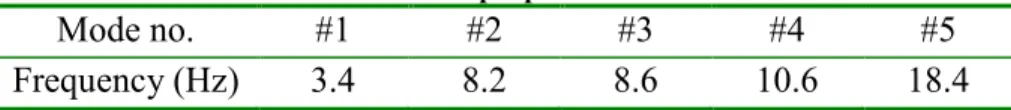
Table 1. Modal properties of the structure
Mode no. #1 #2 #3 #4 #5 Frequency (Hz) 3.4 8.2 8.6 10.6 18.4 3 4 5 6 7 8 9 10 11 12 13 14 15 16 17 18 19 20 21 22 23 24 25 26 27 28 29 30 31 32 33 34 35 36 37 38 39 40 41 42 43 44 45 46 47 48 49 50 51 52 53 54 55
For Peer Review
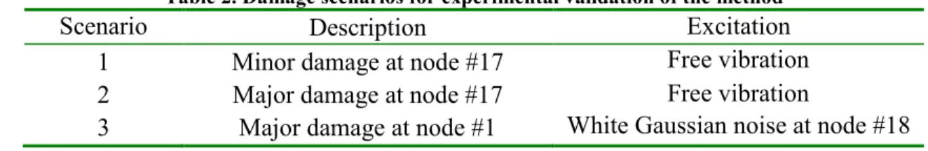
Table 2. Damage scenarios for experimental validation of the method
Scenario Description Excitation
1 Minor damage at node #17 Free vibration
2 Major damage at node #17 Free vibration
3 Major damage at node #1 White Gaussian noise at node #18
3 4 5 6 7 8 9 10 11 12 13 14 15 16 17 18 19 20 21 22 23 24 25 26 27 28 29 30 31 32 33 34 35 36 37 38 39 40 41 42 43 44 45 46 47 48 49 50 51 52 53 54 55 56
For Peer Review
Fig. 1 The areas between the baseline and actual NCED of structural response at a sensor location 3 4 5 6 7 8 9 10 11 12 13 14 15 16 17 18 19 20 21 22 23 24 25 26 27 28 29 30 31 32 33 34 35 36 37 38 39 40 41 42 43 44 45 46 47 48 49 50 51 52 53 54 55
For Peer Review
Fig. 2 Intact and test clusters for a sensor location before and after damage
0.96 0.98 1 0.1 0.15 0.2 0.25 0 1 2 3 4 x 10⁻⁴ DI 1 DI 2 DI 3 intact Damaged 3 4 5 6 7 8 9 10 11 12 13 14 15 16 17 18 19 20 21 22 23 24 25 26 27 28 29 30 31 32 33 34 35 36 37 38 39 40 41 42 43 44 45 46 47 48 49 50 51 52 53 54 55 56
For Peer Review
Fig. 3 The ellipse passing through mT formed by the covariance of the intact cluster. The solid
ellipse is the Mahalanobis distance between the mean values of the clusters conditioning on null hypothesis. The volume under the distribution in the shaded zone is the probability of accepting
the null hypothesis in a hypothesis testing with two DIs
3 4 5 6 7 8 9 10 11 12 13 14 15 16 17 18 19 20 21 22 23 24 25 26 27 28 29 30 31 32 33 34 35 36 37 38 39 40 41 42 43 44 45 46 47 48 49 50 51 52 53 54 55
For Peer Review
Fig. 4 Comparison of Euclidian and Mahalanobis distances when some of the DIs are insensitive to the damage 3 4 5 6 7 8 9 10 11 12 13 14 15 16 17 18 19 20 21 22 23 24 25 26 27 28 29 30 31 32 33 34 35 36 37 38 39 40 41 42 43 44 45 46 47 48 49 50 51 52 53 54 55 56
For Peer Review
Fig. 5 Schematic representation of the proposed algorithm
Choose significance level, α, for hypothesis
testing. (eg. 0.05) Compute NCMHS of response at each sensor location for each test on
the intact structure
Compute the baseline NCMHS for each sensor
location by taking the median of all NCMHS
at the same location
Form the intact cluster by calculating DIs using
the intact NCMHS and baselines
INITIALIZATION
At each node:
1- (p-value) > 1-α
Use or the p-values for damage
localization The structure is intact Yes No Computing NCMHS
of the new data
Form the second cluster by computing
the DIs using the actual NCMHS and the baseline at each
sensor location
Compute and
Perform single one-dimensional one-sided
hypothesis testing on
and and
compute p-values for each sensor location
DETECTION / LOCALIZATION
3 4 5 6 7 8 9 10 11 12 13 14 15 16 17 18 19 20 21 22 23 24 25 26 27 28 29 30 31 32 33 34 35 36 37 38 39 40 41 42 43 44 45 46 47 48 49 50 51 52 53 54 55For Peer Review
(a) (b)
Fig. 6 The experimental setup for testing the proposed algorithm; a) the three-story two-bay structure; b) a sensor next to a connection
x
y
z
1 2 3 10 11 12 4 5 6 7 8 9 13 14 15 16 17 18 3 4 5 6 7 8 9 10 11 12 13 14 15 16 17 18 19 20 21 22 23 24 25 26 27 28 29 30 31 32 33 34 35 36 37 38 39 40 41 42 43 44 45 46 47 48 49 50 51 52 53 54 55 56For Peer Review
(a) (b) (c) (d) (e)
Fig. 7 The first five modes of the laboratory structure from (a) to (e), respectively 3 4 5 6 7 8 9 10 11 12 13 14 15 16 17 18 19 20 21 22 23 24 25 26 27 28 29 30 31 32 33 34 35 36 37 38 39 40 41 42 43 44 45 46 47 48 49 50 51 52 53 54 55
For Peer Review
Fig. 8 MHS and NCMHS of the response at node #17 before and after the occurrence of damage at node #17. The baseline energy distribution is drawn by a thick blue line. Each of the thin lines
corresponds to the energy distribution of an individual test on the structure
0 50 100 150 200 250 300 350 10−4 10−3 10−2 10−1 Frequency (Hz) MHS (log scale)
node # 17 before damage
0 50 100 150 200 250 300 350 10−4 10−3 10−2 10−1 Frequency (Hz) MHS (log scale)
node # 17 after damage
0 50 100 150 200 250 300 350 0 0.2 0.4 0.6 0.8 1 Frequency (Hz) NCMHS
node # 17 before damage
0 50 100 150 200 250 300 350 0 0.2 0.4 0.6 0.8 1 Frequency (Hz) NCMHS
node # 17 after damage
Baseline NCMHS Baseline MHS Baseline MHS Baseline NCMHS 3 4 5 6 7 8 9 10 11 12 13 14 15 16 17 18 19 20 21 22 23 24 25 26 27 28 29 30 31 32 33 34 35 36 37 38 39 40 41 42 43 44 45 46 47 48 49 50 51 52 53 54 55 56
For Peer Review
Fig. 9 MHS and NCMHS of the response at node #14 before and after damage occurrence at node #17. The baseline energy distribution is drawn by a thick blue line. Each of the thin lines corresponds to the energy distribution of an individual test on the structure. Note that node #14 is
adjacent to the location of damage
0 50 100 150 200 250 300 350 10−4 10−3 10−2 10−1 Frequency (Hz) MHS (log scale)
node # 14 before damage
0 50 100 150 200 250 300 350 10−4 10−3 10−2 10−1 Frequency (Hz) MHS (log scale)
node # 14 after damage
0 50 100 150 200 250 300 350 0 0.2 0.4 0.6 0.8 1 Frequency (Hz) NCMHS
node # 14 before damage
0 50 100 150 200 250 300 350 0 0.2 0.4 0.6 0.8 1 Frequency (Hz) NCMHS
node # 14 after damage
Baseline NCMHS Baseline NCMHS Baseline MHS Baseline MHS 3 4 5 6 7 8 9 10 11 12 13 14 15 16 17 18 19 20 21 22 23 24 25 26 27 28 29 30 31 32 33 34 35 36 37 38 39 40 41 42 43 44 45 46 47 48 49 50 51 52 53 54 55
For Peer Review
(a) (b)
Fig. 10 The probability of rejecting the null hypothesis associated with the intact state of each sensor location; a) minor damage at node #17, b) major damage at node #17
1 2 3 4 5 6 7 8 9 10 11 12 13 14 15 16 17 18 0 0.1 0.2 0.3 0.4 0.5 0.6 0.7 0.8 0.9 1 Node no. 1− p −value NCMHS NCPSD 1 2 3 4 5 6 7 8 9 10 11 12 13 14 15 16 17 18 0 0.1 0.2 0.3 0.4 0.5 0.6 0.7 0.8 0.9 1 Node no. 1− p −value NCMHS NCPSD 3 4 5 6 7 8 9 10 11 12 13 14 15 16 17 18 19 20 21 22 23 24 25 26 27 28 29 30 31 32 33 34 35 36 37 38 39 40 41 42 43 44 45 46 47 48 49 50 51 52 53 54 55 56
For Peer Review
(a) (b)Fig. 11 Damage localization using Rβ and comparison between the algorithm’s results when NCPSD is employed for feature extraction instead of NCMHS: a) minor damage at node # 17; b)
major damage at node # 17. In both scenarios the location of damage is more distinguishable when NCMHS is used 1 2 3 4 5 6 7 8 9 10 11 12 13 14 15 16 17 18 10−1 100 101 102 Node no. Rβ NCMHS NCPSD 1 2 3 4 5 6 7 8 9 10 11 12 13 14 15 16 17 18 10−1 100 101 102 103 104 Node no. Rβ NCMHS NCPSD 3 4 5 6 7 8 9 10 11 12 13 14 15 16 17 18 19 20 21 22 23 24 25 26 27 28 29 30 31 32 33 34 35 36 37 38 39 40 41 42 43 44 45 46 47 48 49 50 51 52 53 54 55
For Peer Review
(a) (b)Fig. 12 Sensitivity of each DI to the damage for: (a) the first damage scenario; (b) the second damage scenario
1 2 3 4 5 6 7 8 9 10 11 12 13 14 15 16 17 18 0 0.1 0.2 0.3 0.4 0.5 0.6 Node no. E DI DI 1 DI 2 DI 3 DI 4 1 2 3 4 5 6 7 8 9 10 11 12 13 14 15 16 17 18 0 0.2 0.4 0.6 0.8 1 1.2 1.4 1.6 Node no. E DI DI 1 DI 2 DI 3 DI 4 3 4 5 6 7 8 9 10 11 12 13 14 15 16 17 18 19 20 21 22 23 24 25 26 27 28 29 30 31 32 33 34 35 36 37 38 39 40 41 42 43 44 45 46 47 48 49 50 51 52 53 54 55 56
For Peer Review
(a) (b)
Fig. 13 Damage detection/localization and comparing the results when using MHS vs. PSD as the energy distribution for the third scenario with a major damage at node #1 and white Gaussian
noise excitation: a) the probabilities of rejecting the null hypothesis at each sensor location; b)
β
R ratios at each sensor location
1 2 3 4 5 6 7 8 9 10 11 12 13 14 15 16 17 18 0 0.1 0.2 0.3 0.4 0.5 0.6 0.7 0.8 0.9 1 Node no. 1− p −value NCMHS NCPSD 1 2 3 4 5 6 7 8 9 10 11 12 13 14 15 16 17 18 10−1 100 101 102 103 Node no. Rβ NCMHS NCPSD 3 4 5 6 7 8 9 10 11 12 13 14 15 16 17 18 19 20 21 22 23 24 25 26 27 28 29 30 31 32 33 34 35 36 37 38 39 40 41 42 43 44 45 46 47 48 49 50 51 52 53 54 55
For Peer Review
Fig. 14 Damage detection results for the repaired structure when using MHS vs. PSD 1 2 3 4 5 6 7 8 9 10 11 12 13 14 15 16 17 18 0 0.1 0.2 0.3 0.4 0.5 0.6 0.7 0.8 0.9 1 Node no. 1− p −value NCMHS NCPSD 3 4 5 6 7 8 9 10 11 12 13 14 15 16 17 18 19 20 21 22 23 24 25 26 27 28 29 30 31 32 33 34 35 36 37 38 39 40 41 42 43 44 45 46 47 48 49 50 51 52 53 54 55 56