HAL Id: hal-00504095
https://hal.archives-ouvertes.fr/hal-00504095
Submitted on 19 Jul 2010
HAL is a multi-disciplinary open access
archive for the deposit and dissemination of
sci-entific research documents, whether they are
pub-lished or not. The documents may come from
teaching and research institutions in France or
abroad, or from public or private research centers.
L’archive ouverte pluridisciplinaire HAL, est
destinée au dépôt et à la diffusion de documents
scientifiques de niveau recherche, publiés ou non,
émanant des établissements d’enseignement et de
recherche français ou étrangers, des laboratoires
publics ou privés.
Total Variation regularization enhances regression-based
brain activity prediction
Vincent Michel, Alexandre Gramfort, Gaël Varoquaux, Bertrand Thirion
To cite this version:
Vincent Michel, Alexandre Gramfort, Gaël Varoquaux, Bertrand Thirion. Total Variation
regularization enhances regressionbased brain activity predicregularization. 1st ICPR Workshop on Brain Decoding
-Pattern recognition challenges in neuroimaging - 20th International Conference on -Pattern
Recogni-tion, Aug 2010, Istanbul, Turkey. pp.9-12, �10.1109/WBD.2010.13�. �hal-00504095�
Total Variation regularization enhances regression-based brain activity prediction
Vincent Michel∗†‡, Alexandre Gramfort∗†, Gael Varoquaux ∗†, Bertrand Thirion∗† ∗Parietal team, INRIA Saclay-Ile-de-France, Saclay, France
†CEA, DSV, I2BM, NeuroSpin, Saclay, France ‡Universit´e Paris-Sud 11, Orsay, France
Abstract—While medical imaging typically provides massive amounts of data, the automatic extraction of relevant informa-tion in a given applicative context remains a difficult challenge in general. With functional MRI (fMRI), the data provide an indirect measurement of brain activity, that can be related to behavioral information. It is now standard to formulate this relation as a machine learning problem where the signal from the entire brain is used to predict a target, typically a behavioral variable. In order to cope with the high dimension-ality of the data, the learning method requires a regularization procedure. Among other alternatives, ℓ1regularization achieves
simultaneously a selection of the most predictive features. One limitation of the latter method, also referred to as Lasso in the case of regression, is that the spatial structure of the image is not taken into account, so that the extracted features are often hard to interpret. To obtain more informative and interpretable results, we propose to use the ℓ1 norm of the image gradient,
a.k.a., the Total Variation (TV), as regularization. TV extracts few predictive regions with piecewise constant weights over the whole brain, and is thus more consistent with traditional brain mapping. We show on real fMRI data that this method yields more accurate predictions in inter-subject analysis compared to voxel-based reference methods, such as Elastic net or Support Vector Regression.
Keywords-fMRI; regression; regularization; Total Variation; spatial structure
I. INTRODUCTION
Inferring behavioral information or cognitive states from brain activation images such as those obtained with functional magnetic resonance imaging (fMRI) is a recent neuroimaging data analysis paradigm ? that can provide more sensitive analyzes than standard statistical parametric mapping procedures ?. This approach can be used to assess the involvement of one or several brain regions in certain cognitive or perceptual functions, by evaluating the accuracy of the prediction of a behavioral variable of interest (the target). This inference generally uses a prediction function whose accuracy depends on its ability to use the relevant variables, i.e., the correct brain regions. Importantly, inference methods should simultaneously lead to good prediction performance and provide an interpretable model: the predictive function learned from the data should be as explicit as standard statistical mapping results. This objective is addressed by the TV regression presented in this contribution.
Many methods have been tested for classification or
regression of fMRI activation images (Linear Discriminant Analysis, Support/Relevance Vector Machines, Lasso, Elastic net regression and many others), but in this problem the major bottleneck remains the extraction of predictive information within the brain volume (see ? for a review). In practice, feature selection is important to achieve accurate prediction: when the number of features (voxels) is much larger than the numbers of samples (images), the prediction method overfits the training set, and thus does not generalize well. Besides, feature selection drastically reduces the spatial support of predictive regions, and thus potentially provides a simpler spatial distribution of the predictive features than whole-brain maps.
To date, the most widely used method for feature selection is voxel-based Anova (Analysis of Variance), that evaluates each voxel independently. This is often combined with a Support Vector Machines approach as prediction function. However, it is suboptimal to perform feature selection and parameter estimation procedures separately, and there is a lot of interest in regularization methods that perform both simultaneously.
Let us introduce the following regression model:
y = X w + ǫ (1) where y represents the target data (y ∈ Rn) and w the
parameters to be estimated. The vectorw ∈ Rm
can be seen as an image; m is the number of features (or voxels). The matrix X ∈ Rn×m is the design matrix. Each row is an
m-dimensional sample. The crucial issue here is thatn ≪ m, so that estimatingw is an ill-posed problem. The estimation requires therefore adapted regularization.
A standard approach to perform the estimation of w with regularization uses penalization of the maximum likelihood estimator. This leads to the following minimization problem:
ˆ
w = arg minwky − Xwk
2+ J(w)
(2) whereJ(w) is the penalization term.
The reference method is Elastic net (see ?), which is a combinedℓ1andℓ2penalizationJ(w) = λ1kwk11+λ2kwk22.
Elastic net has two limit cases: λ2 = 0 is the Lasso ?
which yields an extreme sparsity in the selected features, andλ1= 0 corresponds to Ridge regression.
However, such a penalization does not take into account the underlying structure of w, i.e., a spatial 3-dimensional grid in the case of brain images. The main motivation for using this spatial structure is that the predictive information is organized in regions, and not randomly spread across voxels. In this article, we develop an approach for regularized regression based on Total Variation (TV), that we call TV regression. TV ends up providing an estimate w of w withˆ a sparse block structure, from which the regions involved in the cognitive task can be extracted.
Mathematically TV, which has been widely used in image denoising ?, is defined as theℓ1norm of the gradient of the
image: T V (w) = Z ω∈Ω q ▽xw(ω)2+ ▽yw(ω)2+ ▽zw(ω)2dω
In this contribution, the mathematical and implementation details of TV regression are first detailed. It is then applied to an fMRI paradigm that studies object size characterization. Results show that TV outperforms other reference methods, as it yields better prediction performance while providing weights w with an interpretable spatial structure.ˆ
II. METHODS A. Total Variation regression
The computational procedure used for TV regression is based on the gradients of theℓ2 data fidelity term in Eq. (2)
and the computation of the proximity operator associated with the TV penalty.
Definition (Proximity operator). Let J : Rm → R be
a lower semi-continuous, convex function. The proximity operator associated with J and λ ∈ R+ denoted by
proxλJ: Rm→ Rmis given by
proxλJ(w) = arg min
v∈Rm
1
2kv − wk
2
2+ λJ(v) .
In the particular case of TV, the proximity operator is known as the ROF problem ? and recent results ? have shown that it could be solved efficiently with first order iterative procedures. The pseudo code is provided in Al-gorithm 1. For details and proof of convergence of the algorithm see ?. In practice, the stopping condition for the iterative computation of the TV proximity operator is based on the computation of a duality gap. This guarantees the optimality of the solution (it sets the P variable). The number of iterationsN is fixed to 500 as it turns out to lead to an acceptable convergence using the fMRI data presented here. A difficulty specific to fMRI data is the computation of the gradient and divergence over a mask of the brain with correct border conditions. Moreover, with such an irregular domain, the Lipschitz constantL also needs to be estimated on each input data. To do this we use a power method classically used to estimate the spectral norm of a linear operator.
Algorithm 1 Pseudo-code for solving the TV regression Ensure: Let λ > 0 and X be the design matrix. Let Ω
denote the image domain. Let grad : Ω → R3 be a
gradient operator and div : Ω3 → R be the associated
adjoint divergence operator. Let K be the convex set defined by: K = {g : Ω3 s.t. for all ω ∈ Ω, kg(ω)k =
pg1(ω)2+ g2(ω)2+ g3(ω)2 ≤ 1} and ΠK be the
pro-jection operator onto the set K.
Require: Set maximum number of iterations N and P . Compute the spectral norm kXTXk and set µ s.t. 0 <
µ < 2kXTXk−1
. Initialize a ∈ Ω3
with zeros. Compute an upper boundL of the Lipschitz constant of the operator div(grad(·)).
forn = 1 to N do
# Gradient step of the ℓ2 term
v = w + µXT(y − Xw)
# Then compute the TV proximity operator b = a, t = 1 forp = 1 to P do aold= a a = b − 1 µλLgrad(v − µλdiv(b)) a = ΠK(a) told= t t = t+√1+4t2 2 b = a + told−1 t (a − aold) end for w = v − λdiv(a) end for return w B. Performance evaluation
Our method is evaluated with a cross-validation procedure that splits the available data into training and validation sets (here we use a leave-one-subject-out procedure). In the following, (Xl, yl) are a learning set, (Xt, yt) a test set
and yˆt = Xtw refers to the predicted target, where ˆˆ w is
estimated from the training set. The performance of the different regression models is evaluated using ζ, the ratio of explained variance (orR2 coefficient):
ζ(Xl, yl, Xt, yt) =var(yt) − var (yt− ˆyt)
var(yt)
This is the amount of variability in the response that can be explained by the model (perfect prediction yieldsζ = 1, whileζ < 0 if prediction is worse than chance).
C. Competing methods
The TV regression is compared to different reference methods :
• Elastic Net regression, that requires a double
opti-mization, for the two parametersλ1 and λ2. A
cross-validation procedure within the training set is used to optimize these parameters. Here, we use λ1 ∈
{0.2˜λ, 0.1˜λ, 0.05˜λ, 0.01˜λ}, where ˜λ = kXTyk ∞, and
λ2∈ {0.1, 0.5, 1., 10., 100.}.
• Support Vector Regression( SVR) with a linear kernel
(see ?), which is the reference method in neuroimag-ing, due to its robustness in large dimension. The C parameter is optimized by cross-validation in the range 10−3 to101 in multiplicative steps of10.
Both of these methods are used jointly after an Anova-based feature selection as this maximizes their performance. This selection is performed on the training set of each fold in the cross-validation loop, and the optimal number of voxels is selected within the range {50, 100, 250, 500}. The three methods are developed in Python. Both Elastic Net and SVR are freely available in the Scikit-learn package ?.
III. EXPERIMENTS ANDRESULTS A. Experiments on Real Data
We used a real fMRI dataset related to an experiment on the representation of objects, as detailed in ?. During the experiment, ten healthy volunteers viewed objects of three different sizes and four different shapes, with 4 repetitions of each stimulus in each one of 6 sessions. Functional images were acquired on a 3-T MR system with eight-channel head coil (Siemens Trio, Erlangen, Germany) as T2*-weighted echo-planar image (EPI) volumes. Twenty transverse slices were obtained with a repetition time of 2 s (echo time, 30 ms; flip angle, 70◦; 2 × 2 × 2-mm voxels;
0.5-mm gap). Realignment, normalization to MNI space, and General Linear Model (GLM) fit were performed with the SPM5 software. In the present work we used the resulting session-wise parameter estimate images. The four different shapes of objects are pooled across the three sizes, and we are interested in discrimination between sizes. This can be handled as a regression problem, where we aim at predicting the size of an object corresponding to a new fMRI scan. We perform an inter-subjects analysis that relies on subject-specific fixed-effects activations (across repetitions). This yields a total of12 images by subject, with 4 images for each 3 sizes of object. Thus, the dimensions of the real data set are m ∼ 7 × 10⁴
andn = 120 (divided in 3 sizes). We evaluate the performance of the method by cross-validation (leave-one-subject-out), which yields an average rate of explained variance across subjects. This analysis is launched on the whole brain volume.
The parameters of the reference methods are optimized with a leave-one-subject-out cross-validation within the training set, using a three-way grid search in the ranges given before. In the TV regression procedure, the λ parameter is set via the definition of an auxiliary variable α = λ/n where n is the number of images. This scaling makes the setting of the regularization parameter easier and more stable between different datasets.
B. Results on Real Data
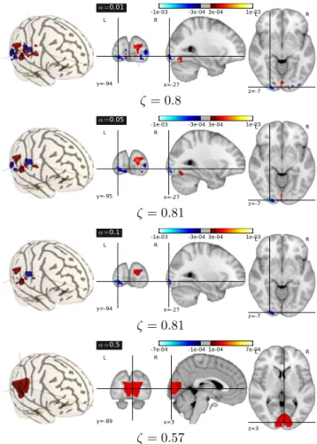
The results found by the three methods are given in Ta-ble I. TV regression outperforms the two alternative methods, yielding an average explained variance of 81%. Moreover, the predictions of TV regression are more stable than the ones of the two reference methods, with a standard deviation of the explained variance two times smaller than the SVR. The weight maps found for different values of the regular-ization parameter λ are shown in Fig.1. It can be seen that, when λ increases, the spatial support of these maps tends to be aggregated in very few clusters within the occipital cortex, and that they have a nearly constant value on these clusters. When λ decreases, the TV regression algorithm is able to create small informative clusters within the occipital cortex, that are comparable to standard activation maps, but where most of the brain regions are shrunk toward 0. By contrast, both reference methods yield uninterpretable maps, with a few informative voxels spread out in the whole occipital cortex, so that it is very difficult to identify meaningful brain structures from these maps.
Table I
SCORES OF EXPLAINED VARIANCE FOR THE DIFFERENT METHODS
Methods mean ζ std ζ max ζ min ζ Time (s) SVR 0.7 0.17 0.92 0.4 151 Elastic net 0.75 0.14 0.96 0.48 2428 TV 0.81 0.08 0.97 0.7 241 All three methods have also been tested in an intra-subject analysis using the same dataset. In that case, they lead to very similar results in terms of performance, although the SVRyields slightly better accuracy than TV regression . This is due to the fact that the voxel-to-voxel correspondence between images is valid in an intra-subject analysis com-pared to an inter-subject analysis. However, the voxel-based approaches still suffer from the limitation that the maps obtained are very hard to interpret.
IV. DISCUSSION
Regularization of voxels loadings significantly increases the generalization ability in regression problems. However, regularization is commonly performed without using the spa-tial structure of the images. The proposed approach performs an adaptive and efficient regularization, while creating in-terpretable weighted maps with regions of constant weights. Thus, the TV regression method fulfills the two requirements that make it suitable for neuroimaging: a good prediction accuracy (equal to or better than the reference methods), and a set of interpretable features, i.e., clusters of similarly tuned voxels. Especially, in the case of a multi-subject study, considering extended regions is expected to compensate for spatial misalignment between individual datasets, hence can better generalize than voxel-based methods. Another asset of the TV regression is that it allows to consider the whole brain in the analysis, without requiring any prior feature selection. Finally, an important feature of our implementation is that it
reduces computation time to a reasonable amount, so that it is not significantly more costly than SVR or Elastic Net in practical settings (i.e., including the cross-validation loops, see Table I).
From a neuroscientific point of view, the selected regions from a whole brain analysis are concentrated in the early visual cortex. This is consistent with the fact that early visual cortex yields highly reliable signals that are discriminative of feature/shape differences between object exemplars, which holds as long as no high-level generalization across images is required (see e.g. ? and ?). Finally, the spatial pattern of this information is stable enough across subjects to be extracted and used to make reliable predictions.
V. CONCLUSION
In this paper we proposed to adapt TV regression for extracting information from brain images. The feature se-lection and model estimation are performed jointly and capture the predictive information present in the data better than alternative methods. A particularly important property of this approach is its ability to create spatially coherent regions with similar weights, yielding interpretable and still informative sets of features. Experimental results show that this algorithm performs particularly well on real data in a multi-subject analysis. These observations demonstrate that TV regression is a powerful tool for understanding brain activity.
Acknowledgements: The authors acknowledge support from the ANR grant ViMAGINE ANR-08-BLAN-0250-02.
L R
y=-94 x=-27
L R
z=-7 -1e-03 -3e-04 3e-04 1e-03 α =0.01 ζ = 0.8 L R y=-95 x=-27 L R z=-7 -1e-03 -3e-04 3e-04 1e-03 α =0.05 ζ = 0.81 L R y=-94 x=-27 L R z=-7 -1e-03 -3e-04 3e-04 1e-03 α =0.1 ζ = 0.81 L R y=-89 x=3 L R z=3 -7e-04 -1e-04 1e-04 7e-04 α =0.5
ζ = 0.57
Figure 1. Maps of weights found by TV regression for different values of the regularization parameter α. When it decreases, the TV regression algorithm creates different clusters of weights with constant values. These clusters are more easily interpretable than voxel-based map (see bellow). Moreover, the clusters are found in the visual cortex, as expected, and show an interesting spatial structure which seems symmetrical: clusters with negative weights are more lateral than clusters with positive weights, and less ventral. The TV regression algorithm is stable for different values of α in the range[0.01, 0.1], has shown by the explained variance ζ.
L R
y=-77 x=-21
L R
z=-12 -3e-02 -5e-03 5e-03 3e-02 svr 500 voxels ζ = 0.7 L R y=-88 x=-24 L R z=-13 -8e-02 -2e-032e-03 8e-02 Elastic net
21 voxels
ζ = 0.75
Figure 2. Maps of weights found by the SVR (up) and Elastic net (bottom) methods. The optimal number of voxels selected by Anova is500, but Elastic netfurther reduces this set to 21 voxels. These voxel-based methods yield features that are difficult to interpret (especially when compared to TV regression), which is related to the fact that they do not consider the spatial structure of the image