Extent of partial ice cover due to carbon cycle feedback in a zonal energy balance model

HAL Id: hal-00304771

https://hal.archives-ouvertes.fr/hal-00304771

HAL is a multi-disciplinary open access archive for the deposit and dissemination of sci-entific research documents, whether they are pub-lished or not. The documents may come from teaching and research institutions in France or abroad, or from public or private research centers.

L’archive ouverte pluridisciplinaire HAL, est destinée au dépôt et à la diffusion de documents scientifiques de niveau recherche, publiés ou non, émanant des établissements d’enseignement et de recherche français ou étrangers, des laboratoires publics ou privés.

Extent of partial ice cover due to carbon cycle feedback

in a zonal energy balance model

C. Huntingford, J. C. Hargreaves, T. M. Lenton, J. D. Annan

To cite this version:

C. Huntingford, J. C. Hargreaves, T. M. Lenton, J. D. Annan. Extent of partial ice cover due to carbon cycle feedback in a zonal energy balance model. Hydrology and Earth System Sciences Discussions, European Geosciences Union, 2003, 7 (2), pp.213-219. �hal-00304771�

Extent of partial ice cover due to carbon cycle feedback in a zonal

energy balance model

C. Huntingford

_{, J.C. Hargreaves}

_{, T.M. Lenton}

_{and J.D. Annan}

2_{Frontier Research System for Global Change, 3173-25 Showa-machi, Kanazawa-ku, Yokohama-shi,Kanagawa, 236-0001, Japan} Also at Proudman Oceanographic Laboratory,Bidston Observatory, Prenton, Merseyside, CH43 7RA, UK

3_{Centre for Ecology and Hydrology, Edinburgh Research Station, Bush Estate, Penicuik,Midlothian, EH26 0QB, UK}

Email for corresponding author: chg@ceh.ac.uk

Abstract

A global carbon cycle is introduced into a zonally averaged energy balance climate model. The physical model components are similar to those of Budyko (1969) and Sellers (1969). The new carbon components account for atmospheric carbon dioxide concentrations and the terrestrial and oceanic storage of carbon. Prescribing values for the sum of these carbon components, it is found that inclusion of a closed carbon cycle reduces the range of insolation over which stable partial ice cover solutions may occur. This highly simplified climate model also predicts that the estimated release of carbon from fossil fuel burning over the next hundred years could result in the eventual melting of the ice sheets.

Keywords: climate, carbon cycle, zonal model, earth system modelling

Introduction

Early advances in the understanding of the Earth’s climate were made through the use of zonally averaged Energy Balance Models (EBMs) (Budyko, 1969; Sellers, 1969). An important result was that the Earth became completely ice covered for modest reductions in insolation and that, for a range of prescribed insolation, multiple solutions are possible including no ice cover, partial ice cover and total ice cover.

In EBMs, there is a single governing equation for the zonal surface temperature; this represents a balance between available radiation (incoming shortwave radiation minus both reflected shortwave radiation and outgoing infrared radiation) and the zonal atmospheric diffusion of heat. The (infrared) radiation emitted back to space is approximated as a linear function of surface temperature. The model is nonlinear, since the prediction of ice cover (a function of surface temperature) has a very strong influence upon surface albedo which in turn influences the outgoing shortwave radiation. A complete review of these simple

zonal climate models, including an analysis of the stability of the equilibrium solutions, is provided by North et al. (1981).

Here a carbon cycle is added to a steady-state zonal energy balance model, with the aim of determining how conserving total carbon in the ocean-atmosphere-land system affects the equilibrium solutions. By experimenting with different amounts of total carbon in the model, some idea of the potential effect on the stability of the climate of net sources or sinks of carbon (caused by processes such as rock weathering, volcanic eruptions and fossil fuel burning) is gained.

This study models how different atmospheric concentrations of carbon dioxide affect the linear approximation between temperature and outgoing infrared radiation (the so-called ‘greenhouse effect’). This adjusts atmospheric temperature, as predicted by the governing thermal equation. The zonal variation in temperature is modelled as influencing carbon storage both within terrestrial ecosystems, and within the ocean. Changes in both

C. Huntingford, J.C. Hargreaves, T.M. Lenton and J. Annan

of these stores of carbon change the atmospheric carbon dioxide concentrations, thereby ‘closing’ the modelled carbon cycle. In the resulting model, as for the original form of the zonal energy balance models, the only input variable is insolation. This, therefore, allows a direct comparison between simulations both with and without a global carbon cycle.

Governing equations

The present numerical model (named Zonal Earth system Underlying Structure, or ZEUS) consists of two key components: the global heat balance and the global carbon cycle. The heat balance components utilise the equations presented by North et al. (1981), with the exception of an

added explicit dependence upon atmospheric CO₂

concentrations. The global carbon cycle comprises a simple terrestrial vegetation and soil model and a description of ocean carbon storage. The atmosphere and land-surface components have a latitudinal (or ‘zonally averaged’) structure. However, the ocean carbon model is currently in a simpler four box form. In this paper, only equilibrium solutions are considered.

SURFACE TEMPERATURE

The energy balance model of surface temperature used here is based upon equations presented by North et al. (1981). At each zonal point (represented throughout this paper by x, the sine of latitude), there is a three-way balance between fluxes of heat dissipated by atmospheric diffusion, infrared radiation emitted to space and absorbed incoming shortwave radiation. It is this energy balance that gives an estimate of surface temperature T(x) (K), and the governing equation is:

(1) Here D (W m–1 _K–1_{) is an atmospheric diffusion coefficient}

for heat, I(x) (W m–2_{) is the rate of emissions of infrared}

radiation to space, S (W m–2_{) is the solar insolation,} µ(x) is

a normalised function that accounts for the mean distribution of radiation according to spatial position (approximated by

µ(x) = 1–0.477*0.5*(3x2 _{– 1) (North and Coakley, 1979)),}

α(x; xs) is the albedo and xs is ice front position. The ice

front position is assumed to be symmetrical in the Northern and Southern hemispheres.

The albedo is given by a two state function, dependent on the presence or absence of ice cover. The particular state is determined by a simple function of temperature, that ice cover exists for surface temperatures less than ten degrees

(centigrade) below freezing point (i.e. T=263.15K at x = x_s). The actual values of albedo are given by:

α(x) = 0.62 for T ≤ 263.15

and α(x) = 0.30 for T > 263.15.

Budyko (1969) suggests that, to a reasonable approximation, infrared radiation emitted to space may be approximated as a linearly increasing function of surface temperature. Parameters associated with such a linearisation implicitly contain a dependence on atmospheric concentrations of ‘greenhouse gases’. It is here that a formal link is made between the global model for surface temperature and the global carbon cycle. An additional term that accounts explicitly for changes in atmospheric CO₂ concentration, c_a (ppm), is added to the linearisation which in turn has been tuned to the current climate. This term is logarithmic in c_a:

I = A + BT – 5.397 ln (2)

where c_a,P (ppm) is atmospheric CO₂ concentration for approximately pre-industrial conditions (here set to 280 ppm) and A (W m–2_{) and B (W m}–2_K–1_{) are constants}

given by A = 203.34W m–2 _{and B = 2.09 W m}–2_K–1_{. The}

values of A and B are those given by North et al. (1981). Such values are assumed to be reasonable for the pre-industrial period, whilst the multiplicative factor of 5.397 is derived directly from a GCM (a function of the response of the complex multi-height atmospheric radiation scheme contained within the Hadley Centre GCM - Shine et al., 1990). From Eqn. (2) it may be seen that if all other conditions are kept constant, then B may be regarded as a climate sensitivity, relating (global) temperature increase for a given change in atmospheric radiative forcing due to

adjustments in the logarithm of atmospheric CO₂

concentration. That is, for fixed solar insolation I, an increase

in atmospheric CO₂ concentration will yield higher

temperatures, T.

Boundary conditions for Eqn. (1) are that dT/dx = 0 at the poles x = ±1. For fixed prescribed atmospheric CO₂ concentration, the above equations (which are nonlinear due to the two-state description of albedo, α) may be solved completely to give zonal values of temperature, T(x). However, the purpose of the work described in this paper is to introduce an interactive carbon cycle and, therefore, atmospheric carbon concentration, c_a, then becomes a variable within the model. Aspects of the global carbon cycle are now introduced.









c

c

TERRESTRIAL CARBON COMPONENT

The terrestrial carbon model is based on the vegetation and soil equations, and associated parameters, given by Lenton (2000). Vegetation carbon density is calculated per unit surface area, C_v (kg C m–2_{), and similarly for soil carbon}

density, C_s (kg C m–2_{). Vegetation carbon content is a balance}

between photosynthesis (generally dominated by the response of leaves in the upper canopy), respiration and litter fall. The dynamic model for vegetation carbon is given by dC_v/dt = k_pC_v,Pf₁(c_a)f₂(T) – k_rf₃(T) C_v – k_tC_v where t is time (yr), k_p (yr–1_{) is a rate constant for photosynthesis,}

C_v,P(kg C m–2_{) is an estimate of vegetation carbon content}

that would be applicable in pre-industrial times, f₁ is a normalised photosynthetic response to atmospheric CO₂ concentration, f₂ is a normalised photosynthetic response to surface temperature T, k_r (yr–1_{) a rate constant for plant}

respiration, f₃ a normalised plant respiration response to temperature and k_t (yr–1_{) a rate constant for litterfall. For the}

equilibrium analyses presented here (indicated by subscript ‘eq’), then:

. (3)

Soil carbon content is a balance between incoming litterfall from vegetation and soil respiration loss. The dynamic equation is given by dC_s/dt = k_tC_v– k_sf₄(T)C_s where C_s (kg C m–2_{) is soil carbon content, k}

s (yr

–1_{) is a soil respiration}

rate constant and f₄ is a normalised soil respiration response to surface temperature. This gives an equilibrium soil carbon content of:

C_s,eq = . (4)

The total carbon content C_land (kg C m–2_{) is the sum of the}

vegetation and soil carbon content (and by definition from Eqns. (3) and (4), a function of atmospheric concentration and surface temperature i.e. C_land(T(x), c_a) = C_v,eq +C_s,eq. At each zonal position where temperature, T, is calculated, (as given by Eqn. (1)), this is applied to solve Eqns. (3) and (4). At each zonal position, fractional land cover, f(x), is based on a dataset of global land cover. Atmospheric CO₂ concentration, c_a, is assumed to be well mixed and invariant with position. The total vegetation cover, C (GtC) therefore satisfies:

C = (5)

where N is the number of zonal bands used in the calculation of Eqn. (1) (set arbitarily in this study as 73), ∆x (m2_{) is the}

area of each zonal band and v₁ converts to units of GtC.

OCEAN CARBON COMPONENT

The ocean model is based on the four box structure presented by Knox and McElroy (1984), with adjustments introduced by Lenton (2000). The four boxes are warm low-latitude surface water ‘w’, cold high-latitude surface water ‘c’, intermediate water ‘i’ and deep water ‘d’. A fraction 0.15 of the ocean surface area is assigned to the cold surface water box, and 0.85 to the warm surface water box. The surface boxes are both 100m deep. The intermediate box is prescribed as 1000m deep. The ocean circulation and biological parameters are held constant at the values given in Lenton (2000). Each box contains three tracers: nitrate, alkalinity and total inorganic carbon, T_CO2 (mol kg–1_{). Total}

nitrate and alkalinity are held constant, and hence their concentrations in each box are constant. Only T_CO2 can vary. The model gives equilibrium solutions for total carbon content of the ocean, c (GtC) given atmospheric CO₂

concentration, c_a, and a corresponding latitudinal

temperature profile.

Temperatures for the two surface ocean boxes are calculated from the latitudinal temperature profile by area-weighted averaging, taking into account the ocean area within each band and the asymmetry of the distribution of land between the hemispheres. The thermodynamic dissociation constants for seawater are calculated for each surface box, as functions of temperature and fixed salinity (using the same functions as Lenton, 2000). The T_CO2 in each ocean box is calculated using the flux relationships between the boxes (Lenton, 2000) as well as the relations between T_CO2 and the partial pressure of carbon dioxide (P_CO2, (ppm)) from Kilho Park (1969). In previous work, where solutions for a single water mass were required (e.g. Peng et al., 1987), T_CO2 and P_CO2, calculations have used ad-hoc iterative methods. Here, equations for all four boxes have to be solved together and, with this additional complexity, the direct iteration is found to not converge reliably. Instead, the well-known method of False Position (Press et al., 1994: Section 9.2) is employed to find T_CO2 in all the boxes. The method is applied to hydrogen ion activity in the Kilho Park relations, and to P_CO2 in the warm surface box to solve the simultaneous flux equations. The four T_CO2 values are then multiplied by the volume of the relevant ocean boxes and summed to give the total carbon in the ocean. A units conversion gives this total in GtC, named as C . CARBON CYCLE CLOSURE AND SOLUTIONS

The total carbon in the land-ocean-atmospheric system, CTot_,

requires adding the land surface carbon to the ocean carbon and atmospheric carbon (given by C = v₂c_a and v₂ is a units conversion to GtC). That is CTot _{= C + C + C .}

k_tC_v,eq k_sf₄ Tot land v C T N i land

∑

[

]

C. Huntingford, J.C. Hargreaves, T.M. Lenton and J. Annan

The main purpose of this study is understanding how the constraint of maintaining a fixed quantity of carbon within the system (i.e. CTot _{is kept constant) adjusts predictions of}

ice front position for perturbed insolation, compared to earlier simulations that include thermal behaviour only. From the equations of the original thermal model, ice front position (which may have multiple solutions) may be expressed as having the functional form

x_s = x_s (S,c_a). (6)

For the introduction of the carbon cycle, Eqn. (6) is still used, but now c_a requires calculation as an implicit variable and satisfying:

v₂c_a = CTot _{– C (T(x), c}

a) – C (T(x), ca) (7)

where

T(x) = T(S,c_a). (8)

Equations (7) and (8) are solved for both c_a and T as a function of prescribed values of CTot _{and S and so, with the}

carbon cycle introduced, now ice front position has dependencies of:

x_s = x_s(CTot_{, S) (9)}

This paper requires a method to compare how ice front position varies as a function of insolation, S, for solutions

both without a carbon cycle (using Eqn. (6),with c_a

prescribed) and for solutions with a carbon cycle (using Eqn. (9), with CTot _{prescribed). To achieve this, the following}

algorithm is adopted. Starting with the original solutions without a carbon cycle, for a given value of S (called S₀ say), then a solution (or possibly multiple solutions) for ice extent, x_s, is calculated. The associated profile of temperature is then applied to the land surface and oceanic models, and with the prescribed value of c_a gives a value of total carbon, CTot_{. This value is supplied to Eqn. (9). Solving both Eqns.}

(6) and (9) for varying values of S away from the original prescribed value will yield two trajectories that intersect at S = S_o. Comparison of these two solutions for varying insolation demonstrates the impact of the global carbon cycle.

Results and discussion

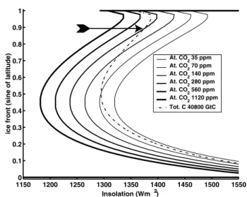
Results are similar to those of North et al. (1981); their

Figure 8 is reproduced with fixed atmospheric CO₂

concentration of c_a = 280 ppm (see the appropriate

continuous line in Fig. 1 corresponding to this value of c_a).

Using the temperature profile calculated for S₀ = 1376 Wm–2 _{(a value of insolation representative of the present}

time), corresponding values of land and ocean carbon are calculated, added to the atmospheric carbon content giving a value of total carbon content of close to 40 800 GtC. This compares well with estimates for the pre-industrial Earth, and is about 400 GtC more than in the simpler box model of Lenton (2000) due to greater ocean carbon storage. This value of CTot _{is then used to create a second set of values for}

x_s, all for this fixed value of carbon within the land-atmosphere-ocean system, and again for varying insolation. This solution is the dashed line in Fig. 1. By definition, the solutions are identical at S = S₀, and this point is indicated by the arrow in Fig. 1. The predicted ice front position under pre-industrial conditions (S₀ = 1376 Wm–2 _{and c}

a = 280 ppm)

is x_s = 0.89, corresponding to 63 degrees N/S. This is above the Southern tip of Greenland (60N) although rather icy for the Earth as a whole. Given the complex orography and unevenness of ice distribution on the Earth (compared with the simplicity of this model), this implies that the model is acceptably well tuned. To achieve such tuning, the atmospheric diffusion co-efficient, D, is set as 0.35 W m–1_K–1_.

Away from the point of intersection, the solutions with CO₂ fixed at 280 ppm, and with constant total carbon of 40 800 GtC, diverge. The total carbon curve crosses several of the constant CO₂ concentration lines. Close to the ice-free state the CO₂ concentration is about 400 ppm, whereas

Tot

land Totocean

1150 1200 1250 1300 1350 1400 1450 1500 1550 0 0.1 0.2 0.3 0.4 0.5 0.6 0.7 0.8 0.9 1 Insolation (Wm 2)

ice front (sine of latitude)

At. CO 2 35 ppm At. CO₂ 70 ppm At. CO 2 140 ppm At. CO 2 280 ppm At. CO₂ 560 ppm At. CO 2 1120 ppm Tot. C 40800 GtC

Fig. 1. Positions of the ice front at different values of insolation. These are for fixed atmospheric CO₂ concentrations, c_a, of 35, 70, 140, 280, 560, and 1120 ppm (thereby overriding the carbon cycle elements in the model, and reducing the model to that of previous authors), and for a fixed value of CTot _{= 40 800 GtC in the}

ocean-atmosphere-land system, estimated for pre-industrial CO2 =

280 ppm and present S = 1376 Wm–2_{. The 280 ppm and 40 800 GtC}

for high ice cover values the CO₂ concentration gets as low as 50 ppm. It has been shown (North et al., 1981) that the only stable solutions for zonal energy balance models are those where the gradient for the plot as shown in Fig. 1 is non-negative (i.e. dx_s/dS > 0). In this regime, for constant total carbon of CTot _{=40 800 GtC, the CO}

2 concentration

varies from about 350 ppm for small ice cap solutions to about 70 ppm for large ice caps. This stable part of the curve is considerably steeper than the same part of the constant CO₂ curves. Studies with time-varying energy balance models (North and Coakley, 1979; North and Cahalan, 1981) have shown that a steeper slope corresponds to increased sensitivity to random perturbations, with both larger fluctuations and longer return times to equilibrium. It is also evident from Fig. 1 that, for the results with total carbon conserved, the range of possible insolation for which stable solutions exist is reduced and the point of transition to the snowball state occurs when there is less ice. Thus, the redistribution of carbon within the ocean-atmosphere-land system acts as a net positive feedback on changes in the partial ice cover solution of the model (atmospheric CO₂ tends to increase and thereby enhances the greenhouse effect with decreasing ice cover, and similarly to decrease with increasing ice cover).

In reality, total carbon in the ocean-atmosphere-land system can vary due to natural processes (e.g. exchange of

carbon with ocean sediments, volcanic input, rock weathering) as well as anthropogenic fossil fuel burning. Hence the numerical experiments are repeated over the stable region for a range of different total carbon values (39 800 GtC to 43 800 GtC). These results are shown by the dashed lines in Fig. 2. The c_a = 280 ppm curve, is shown for comparison (continuous line). For a greater quantity of total carbon in the system, the curves describing the locus of stable solutions are shifted to lower values of insolation. This reflects the fact that increased atmospheric CO₂ reduces radiation loss, and as such, lower values of insolation are required to maintain the same ice front position. For increased total carbon there is also a slight decrease in the gradient of the curves and an increase in the possible ice cover that can occur before a snowball state is induced.

Given current fossil fuel burning, it is interesting to consider the effect on the solutions of changes in total carbon at constant insolation. Starting from the present day solution with S₀ = 1376 W m–2_{, x}

s = 0.89, Fig. 2 shows that an increase

of total carbon of the order of 1000 GtC (whilst retaining S₀ = 1376 W m–2_{) will cause collapse to the ice-free state. That}

is, in Fig. 2 there are no small ice cover solutions for S₀ = 1376 W m–2 _{and C}Tot _{=41 800 GtC. The estimated fossil fuel}

reserves are about 4000 GtC, of which about 200 GtC have been emitted thus far. Following, for example, the IS92a ‘business as usual’ scenario, more than 1000 GtC will have

1220 1240 1260 1280 1300 1320 1340 1360 1380 1400 1420 0.5 0.6 0.7 0.8 0.9 1 Insolation (Wm−2)

ice front (sine of latitude)

Tot. C 39800 GtC Tot. C 40800 GtC Tot. C 41800 GtC Tot. C 42800 GtC Tot. C 43800 GtC At. CO₂ 280 ppm

Fig. 2. Partial ice cover solutions at different values of insolation. This is for different values of fixed total carbon CTot _{in the ocean-atmosphere-land system, and at fixed atmospheric CO}

2 of 280 ppm. At the

points of intersection with the CO2 = 280 ppm curve, the solutions with and without the carbon cycle are

C. Huntingford, J.C. Hargreaves, T.M. Lenton and J. Annan

been emitted by 2100. Thus, in this simple model, human activities could remove the small ice cap solution and shift the system to the ice-free state. A significant reduction in solar luminosity would then be required to get back any ice cover. The steady state model gives no information about transient behaviour, and it does not capture ice sheet dynamics. However, the equilibrium response of the model to increased total carbon can be compared qualitatively with current concerns that the Greenland ice sheet at least may melt under sustained global warming.

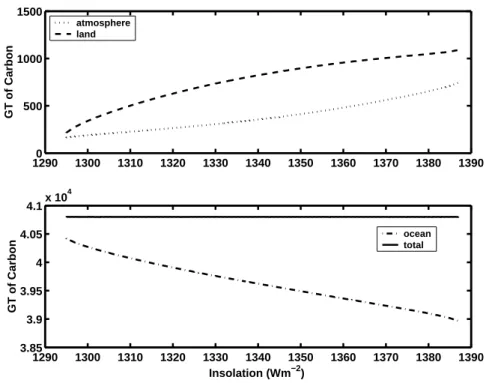
Figure 3 shows for the stable partial ice cover solution, how the apportioning of carbon between the ocean, atmosphere and land varies with insolation, when the total carbon is fixed at 40 800 GtC. The oceanic carbon content decreases with increasing insolation, and this carbon is taken up by the land and to a lesser extent by the atmosphere. Ocean carbon storage decreases with increasing insolation (corresponding to decreasing ice cover) because temperature increases and this reduces the solubility of carbon dioxide. Land carbon storage increases due to a beneficial effect of increasing atmospheric carbon dioxide concentration on photosynthesis and hence on net primary production (in some zonal regions there is also a beneficial effect of warming on land carbon storage). Overall, changes in ocean carbon storage generate positive feedback on changes in solar forcing; changes in land carbon storage generate a

counteracting negative feedback, but the two do not cancel out. Hence a net positive feedback remains whereby atmospheric carbon dioxide concentrations increase as insolation increases.

Conclusions

This paper examines how adding a carbon cycle to a zonal energy balance model affects predictions of planetary states involving partial ice cover. The model has been tuned initially such that for near present day conditions of solar insolation and atmospheric carbon dioxide concentrations, small ice cover solutions (that are known from analysis by other authors to be stable) are predicted. For model solutions with and without the carbon cycle that intersect at

pre-industrial values of insolation and atmospheric CO₂

concentration, the carbon cycle is found to reduce the range of insolation values, S, for which such partial ice cover solutions can exist. In a partial ice cover state, the model which conserves total carbon is considerably more sensitive to changes in insolation. Thus, the system collapses more readily to either a snowball Earth or ice-free state (corresponding, respectively, to either a decrease or increase in incoming planetary radiation). Starting at present day luminosity and pre-industrial CO₂ concentration, increasing the total carbon in the system by about 1000 GtC, e.g. due

Fig. 3. Carbon storage in the ocean, atmosphere and land surface as a function of insolation, for the stable partial ice cover solution and a total carbon content of 40 800 GtC. (This solution corresponds to the dot-dash line in Fig. 1, passing through the present day solution as marked by an arrow in that Figure).

12900 1300 1310 1320 1330 1340 1350 1360 1370 1380 1390 500 1000 1500 GT of Carbon atmosphere land 1290 1300 1310 1320 1330 1340 1350 1360 1370 1380 1390 3.85 3.9 3.95 4 4.05 4.1x 10 4 Insolation (Wm−2) GT of Carbon ocean total

to fossil fuel burning, causes the small ice-cap solution to collapse to the ice-free state.

The assumption of constant total carbon in the ocean-atmosphere-land system is reasonably accurate (in the absence of human intervention), on timescales of up to 103

years. However, at timescales of 103 _{years, exchange of}

carbon with ocean sediments and the weathering of carbonate rocks can alter the ocean-atmosphere-land carbon reservoir size significantly (such interactions generally operate as negative feedbacks on atmospheric carbon dioxide (Archer et al., 1998)). For even longer periods of order 105 _{years, volcanic and metamorphic CO}

2 input and

CO₂ output due to silicate weathering (itself a function of temperature and atmospheric CO₂ concentration) followed by carbonate deposition, can also alter the surface carbon reservoir size. Silicate weathering generally provides a negative feedback on changes in atmospheric carbon dioxide and global temperature (Walker et al., 1981).

To provide some insight into possible changes in planetary ice coverage as a consequence of changes in total carbon within the land-atmosphere-ocean carbon pool, solutions are presented for a range of such total carbon values. Whether the equilibrium solutions presented here are actually realised, or are simply states that the planetary system asymptotes towards, will depend on the balance of any rates of change in total carbon with the timescales implicit in ice sheet dynamics.

Acknowledgement

Funding for this research from both the Centre for Ecology and Hydrology Integrating Fund and the NERC Earth System Modelling Initiative (NESMI) is gratefully acknowledged.

References

Archer, D., Kheshgi, H. and Maier-Reimer, E., 1998. Dynamics of fossil fuel CO₂ neutralization by marine CaCO₃. Global

Biogeochem. Cycles, 12, 259–276.

Budyko, M.I., 1969. The effect of solar radiation variations on the climate of the Earth. Tellus, 21, 611–619.

Kilho Park, P., 1969. Oceanic CO₂ system: an evaluation of ten methods of investigation. Limnol. Oceanography 2, 179–186. Knox, F. and McElroy, M.B., 1984. Change in atmospheric CO₂: influence of the marine biota at high latitude. J. Geophys Res., 89, 4629–4637.

Lenton, T.M., 2000. Land and ocean carbon cycle feedback effects on global warming in a simple Earth system model. Tellus,52B, 1159–1188.

North, G.R. and Coakley, J.A., 1979. Differences between seasonal and mean annual energy balance model calculations of climate and climate sensitivity. J. Atmos. Sci., 36, 1189–1204. North, G.R. and Cahalan, T.J., 1981. Predictability in a solvable

stochastic climate model. J. Atmos. Sci. 38, 504–513. North, G.R., Cahalan, R.F. and Coakley, J.A., 1981. Energy

balance climate models. Review of Geophys. and Space Phys., 19, 91–121.

Peng, T-H., Takahashi, T., Broecker, W.S. and Olafsson, J., 1987. Seasonal variability of carbon dioxide, nutrients and oxygen in the northern North Atlantic surface water: observations and a model. Tellus, 39B, 439–458.

Press. W.H., Teukolsky, S.A., Vetterling, W.T. and Flannery, B.P., 1994. Numerical recipes in Fortran: the art of scientific

computing. Cambridge University Press, Cambridge, UK

Sellers, W.D., 1969. A global climate model based on the energy balance of the earth-atmosphere system. J. Appl. Meteorol., 8, 386–400.

Shine, K., Derwent, R., Wuebbles, D. and Morcette, J.J., 1990. Radiative forcing of climate. In: Climate change. The IPCC

scientific assessment, J. Houghton, G. Jenkins, J. Ephraums,

(Eds.), Cambridge University Press, Cambridge, UK, 45–68. Walker, J. C. G., Hays, P. B. and Kasting, J. F., 1981. A negative

feedback mechanism for the long-term stabilisation of Earth’s surface temperature. J. Geophys. Res., 86, 9776–9782.