HAL Id: hal-01777169
https://hal.archives-ouvertes.fr/hal-01777169
Submitted on 24 Apr 2018
HAL is a multi-disciplinary open access
archive for the deposit and dissemination of
sci-entific research documents, whether they are
pub-lished or not. The documents may come from
teaching and research institutions in France or
abroad, or from public or private research centers.
L’archive ouverte pluridisciplinaire HAL, est
destinée au dépôt et à la diffusion de documents
scientifiques de niveau recherche, publiés ou non,
émanant des établissements d’enseignement et de
recherche français ou étrangers, des laboratoires
publics ou privés.
Scikit-SpLearn : a toolbox for the spectral learning of
weighted automata compatible with scikit-learn
Denis Arrivault, Dominique Benielli, François Denis, Rémi Eyraud
To cite this version:
Denis Arrivault, Dominique Benielli, François Denis, Rémi Eyraud. Scikit-SpLearn : a toolbox for the
spectral learning of weighted automata compatible with scikit-learn. Conférence francophone sur l’
Apprentissage Aurtomatique, Jun 2017, Grenoble, France. �hal-01777169�
Scikit-SpLearn : a toolbox for the spectral learning of weighted
automata compatible with scikit-learn
∗†
Denis Arrivault
1, Dominique Benielli
1, Fran¸cois Denis
2, et R´
emi Eyraud
21
LabEx Archim`
ede, Aix-Marseille University, France
2
QARMA team, Laboratoire d’Informatique Fondamentale de Marseille, France
R´
esum´
e
Scikit-SpLearn is a Python toolbox for the spectral learning of weighted automata from a set of strings, licensed under Free BSD, and compatible with the well-known scikit-learn toolbox. This paper gives the main formal ideas behind the spectral learning algorithm and details the content of the toolbox. Use cases and an experimental section are also provided.
Mots-clef : Toolbox, Spectral Learning, Weighted
Au-tomata
1
Introduction
Grammatical inference is a sub-field of machine lear-ning that mainly focuses on the induction of gram-matical models such as, for instance, finite state ma-chines and generative grammars. However, the core of this field may appear distant from mainstream machine learning : the methods, algorithms, approaches, para-digms, and even mathematical tools used are usually not the ones of statistical machine learning.
There exists one important exception to this obser-vation : the recent developments of what is called spec-tral learning are building a bridge between these two facets of machine learning. Indeed, by allowing the use of linear algebra in the context of finite state machine learning, tools of statistical machine learning are now usable to infer grammatical formalisms.
The initial idea of spectral learning is to des-cribe finite state machines using linear
representa-∗This work was supported in part by the LabEx Archim`ede
of the Aix-Marseille University (ANR-11-LABX-0033). This pu-blication only reflects the authors’ views.
†This paper was published at the Conf´erence sur
l’APpren-tissage (CAp) 2017 (French Machine Learning Conference).
A similar paper concerning a preliminary version of the tool-box, called Sp2Learn have been published at the 13th In-ternational Conference on Grammatical Inference in October 2016 [ABDE16].
tions : instead of sets of states and transitions, these equivalent models are made of vectors and ma-trices [BR88]. The class of machines representable with these formalisms is the one of Weighted Automata (WA)1 [Moh09], sometimes called multiplicity
auto-mata [BBB+96], that are a strict generalization of
Pro-babilistic Automata (PA) [Sch61], of Hidden Markov Models (HMM) [DDE05], and of Partially Observable Markov Decision Processes (POMDP) [TJ15] .
The corner stone of the spectral learning approach is the use of what is called the Hankel matrix. In its classical version, this bi-infinite matrix has rows that correspond to prefixes and columns to suffixes : the va-lue of a cell is then the weight of the corresponding sequence in the corresponding WA. Importantly, the rank of this matrix is the number of states of a minimal WA computing the weights : this allows the construc-tion of this automaton from a rank factorizaconstruc-tion of the matrix [BCLQ14].
Following this result, the behavior of the spectral learning algorithm relies on the construction of a finite sub-block approximation of the Hankel matrix from a sample of sequences. Then, using a Singular Value De-composition of this empirical Hankel matrix, one can obtain a rank factorization and thus a weighted auto-maton.
From the seminal work of Hsu et al. [HKZ09] and Bailly et al. [BDR09], important developments have been achieved. For example, Siddiqi et al. [SBG10] ob-tain theoretical guaranties for low-rank HMM ; A PAC-learning result is provided by Bailly [Bai11] for stochas-tic weighted automata ; Balle et al. [BCLQ14] extend the algorithm to variants of the Hankel matrix and show their interest for natural language processing ; Ex-tensions to the spectral learning of weighted tree auto-mata have been published by Bailly et al. [BHD10].
In the context of this great research effervescence,
1. Only WA whose weights are real numbers are considered in this work.
we felt that an important piece was missing which would help the widespread adoption of spectral lear-ning techniques : an easy to use and to install program with broad coverage to convince non-initiated resear-chers about the interest of this approach. This is the main motivation behind the project of the scikit Spec-tral Learning (Scikit-SpLearn) Python toolbox2 that
this paper presents. Indeed, this software contains se-veral variants of the spectral learning algorithm, toge-ther with optimized data structures (for instance an implementation of weighted automata), and is compa-tible with the internationally known scikit-learn tool-box [PVG+11].
We notice that a code for 3 methods of moments, in-cluding a spectral learning algorithm, is available at https ://github.com/ICML14MoMCompare/spectral-learn. However, this code was designed for a research paper and suffers many limitations, as for instance only a small number of data sets, the one studied in the ar-ticle, can be used easily.
Section 2 gives formal details about the spectral lear-ning of weighted automata. Section 3 carefully des-cribes the toolbox content and provides use cases. Some experiments showing the potential of Scikit-SpLearn are given in Section 4, while Section 5 concludes by giving ideas for future developments.
2
Spectral learning of weighted
automata
2.1
Weighted Automata
A finite set of symbols is called an alphabet. A string over an alphabet Σ is a finite sequence of symbols of Σ. Σ∗ is the set of all strings over Σ. The length of a string w is the number of symbols in the string. We let
ϵ denote the empty string, that is the string of length
0. For any w ∈ Σ∗, let pref (w) = {u ∈ Σ∗ : ∃v ∈ Σ∗, uv = w} be its set of prefixes, suff(w) = {u ∈ Σ∗:
∃v ∈ Σ∗, vu = w} be its set of suffixes, and fact(w) =
{u ∈ Σ∗ :∃l, r ∈ Σ∗, lur = w} be the set of factors of
w (sometime called the set of substrings).
The following definitions are adapted from Mohri [Moh09] :
D´efinition 1 (Weighted automaton) A weighted automaton (WA) is a tuple ⟨Σ, Q, I, F, T , λ, ρ⟩ such that : Σ is a finite alphabet ; Q is a finite set of states ;T : Q × Σ × Q → R is the transition function ;
2. A previous version of the toolbox, not compatible with scikit-learn, was released as a toolbox for the Sequence PredIc-tion ChallengE (SPiCe), an on-line competiPredIc-tion [BEL+16].
λ : Q→ R is an initial weight function ; ρ : Q → R is a final weight function.
A transition is usually denoted (q1, σ, p, q2) instead of
T (q1, σ, q2) = p. We say that two transitions t1 =
(q1, σ1, p1, q2) and t2 = (q3, σ2, p2, q4) are consecutive
if q2= q3. A path π is an element ofT∗made of
conse-cutive transitions. We denote by o[π] its origin and by
d[π] its destination. The weight of a path is defined by µ(π) = λ(o[π])× ω × ρ(d[π]) where ω is the
multiplica-tion of the weights of the constitutive transimultiplica-tions of π. We say that a path (q0, σ1, p1, q1) . . . (qn−1, σn, pn, qn)
reads a string w if w = σ1. . . σn. The weight of a string
w is the sum of the weights of the paths that read w.
A series r over an alphabet Σ is a mapping r : Σ∗→ R. A series r over Σ∗is rational if there exists an integer
k≥ 1, vectors I, T ∈ Rk, and matrices M
σ∈ Rk×k for
every σ∈ Σ, such that for all u = σ1σ2. . . σm∈ Σ∗,
r(u) = IMuT = IMσ1Mσ2. . . MσmT
The triplet⟨I, (Mσ)σ∈Σ, T⟩ is called a k-dimensional
linear representation of r. The rank of a rational series r is the minimal dimension of a linear representation
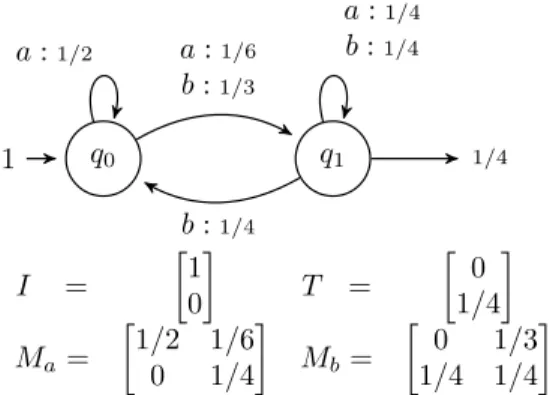
of r. Linear representations are equivalent to weigh-ted automata where each coordinate corresponds to a state, the vector I provides the initial weights (i.e. the values of function λ), the vector T is the terminal weights (i.e. the values of function ρ), and each ma-trix Mσcorresponds to the σ-labeled transition weights
(Mσ(q1, q2) = p⇐⇒ (q1, σ, p, q2) is a transition). q0 1 q1 a :1/6 b :1/3 a :1/2 1/4 a :1/4 b :1/4 b :1/4 I = [ 1 0 ] T = [ 0 1/4 ] Ma = [ 1/2 1/6 0 1/4 ] Mb= [ 0 1/3 1/4 1/4 ]
Figure 1 – A weighted automaton and the equivalent linear representation.
In what follows, we will confound the two notions and consider that weighted automata are defined in terms of linear representations.
A particular kind of WA is of main interest in the spectral learning framework : a weighted automata A
is stochastic if the series r it computes is a probabi-lity distribution over Σ∗, i.e. ∀x ∈ Σ∗, r(x) ≥ 0 and
∑
x∈Σ∗r(x) = 1. These WA enjoy properties that are
important for learning. For instance, in addition to the probability of a string r(x), a WA can compute the probability of a string to be a prefix rp(x) = r(xΣ∗),
or to be a suffix rs(x) = r(Σ∗x). It can be shown that
the rank of the series r, rp, and rsare equal [BCLQ14].
Other properties of stochastic WA are of great interest for spectral learning but it is beyond the scope of this paper to describe them all. We refer the Reader to the work of Balle et al. [BCLQ14] for more details.
Finally, stochastic weighted automata are rela-ted to other finite state models : they are strictly more expressive than Probabilistic Automata [DEH06] (which are equivalent to discrete Hidden Markov Mo-dels [DDE05]) and thus than Deterministic Probabilis-tic Automata [CO94].
2.2
Hankel matrices
The following definitions are based on the ones of Balle et al.[BCLQ14].
D´efinition 2 Let r be a rational series over Σ. The Hankel matrix of r is a bi-infinite matrix H∈ RΣ∗×Σ∗ whose entries are defined as H(u, v) = r(uv) for any u, v ∈ Σ∗. That is, rows are indexed by prefixes and columns by suffixes.
For obvious reasons, only finite sub-blocks of Hankel matrices are going to be of interest. An easy way to define such sub-blocks is by using a basisB = (P, S), whereP, S ⊆ Σ∗. We write p = |P| and s = |S|. The sub-block of H defined byB is the matrix HB∈ Rp×s
with HB(u, v) = H(u, v) for any u∈ P and v ∈ S. We may just write H if the basisB is arbitrary or obvious from the context.
In the context of learning weighted automata, the focus is on a particular kind of bases. They are called
closed bases : a basis B = (P, S) is prefix-closed3 if there exists a basisB′ = (P′,S) such that P = P′Σ′, where Σ′ = Σ∪ {ϵ}. A prefix-closed basis can be par-titioned into |Σ| + 1 blocks of the same size (a given string may belong to several blocks) : given a Hankel matrix H and a prefix-closed basis B = (P, S) with
P = P′Σ′, we have, for a particular ordering of the
elements ofP :
HB⊤ = [Hϵ⊤|Hσ⊤1|Hσ⊤2| . . . |Hσ⊤
|Σ|]
3. Similar notions of closure can be designed for suffix and factor.
where Hσare sub-blocks defined over the basis (P′σ,S)
such that Hσ(u, v) = H(uσ, v). The notation uses here
means that HB⊤ can be restricted to each of the other sub-blocks.
The rank of a rational series r is equal to the rank of its Hankel matrix H which is thus the number of states of a minimal weighted automaton that represents r. The rank of a sub-block cannot exceed the rank of H and we are interested by full rank sub-blocks : a basis
B is complete if HB has full rank, that is rank(HB) =
rank(H).
We will consider different variants of the classical Hankel matrix H of an absolutely convergent series r, i.e. ∑w|r(w)| converges :
— Hpis the prefix Hankel matrix, where Hp(u, v) =
r(uvΣ∗) =∑wr(uvw) for any u, v ∈ Σ∗. In this case rows are indexed by prefixes and columns by factors.
— Hsis the suffix Hankel matrix, where Hs(u, v) =
r(Σ∗uv) =∑wr(wuv) for any u, v ∈ Σ∗. In this matrix rows are indexed by factors and columns by suffixes.
— Hf is the factor Hankel matrix, where Hf(u, v) =
∑
w1,w2r(w1uvw2)
4 for any u, v ∈ Σ∗. In this
matrix both rows and columns are indexed by factors.
2.3
Hankel matrices and WA
We consider a rational series r, H its Hankel matrix, and A =⟨I, (Mσ)σ∈Σ, T⟩ a minimal WA computing r.
We suppose that A has n states.
We first notice that A induces a rank factorization of
H : we have H = P S, where P ∈ RΣ∗×n is such that
its uth row equals I⊤M
u, and similarly S ∈ Rn×Σ
∗
is such that its vth column is M
vT . Similarly, given a
sub-block HBof H defined by the basisB = (P, S) we have HB = PBSB where PB ∈ RP×n and S
B ∈ Rn×S
are restrictions of P and S on P and S, respectively. Besides, if B is complete then HB = PBSB is a rank factorization.
Moreover, the converse occurs : given a sub-block HB of H defined by the complete basisB = (P, S), one can compute a minimal WA for the corresponding rational series r using a rank factorization P S of HB. Let Hσbe
the sub-block of the prefix closure of HBcorresponding to the basis (Pσ, S), and let hP,ϵ∈ RP denotes the p-dimensional vector with coordinates hP,ϵ(u) = r(u), and hϵ,S the s-dimensional vector with coordinates 4. Note that even if r is a rational stochastic language, the series w→ r(Σ∗wΣ∗), i.e. the probability that w appears as a
hϵ,S(v) = r(v). Then the WA A = ⟨I, (Mσ)σ∈Σ, T⟩,
with I⊤ = h⊤ϵ,SS+, T = P+hP,ϵ, and Mσ = P+HσS+,
is minimal for r [BCLQ14]. As usual, N+ denotes the
Moore-Penrose pseudo-inverse of a matrix N .
2.4
Learning weighted automata using
spectral learning
The core idea of the spectral learning of weighted automata is to use a rank factorization of a complete sub-block of the Hankel matrix of a target series to induce a weighted automaton.
Of course, in a learning context, one does not have access to the Hankel matrix : all that is avai-lable is a (multi-)set of strings LS = {x1, . . . , xm},
usually called a learning sample. The learning process thus relies on the empirical Hankel matrix given by
ˆ
HB(u, v) = ˆPLS(u, v) whereB is a given basis and ˆPLS
is the observed frequency of strings inside LS. Hsu et al. [HKZ09] proves that with high probability we have
||HB− ˆHB||F ≤ O(√1m) (see Denis et al. [DGH16] for
other concentration bounds).
In the learning framework we are considering, we suppose that there exists an unknown rational series
r of rank n and we want to infer a WA for r. We are
assuming that we know a complete basis B = (P, S) and have access to a learning sample LS. Obviously, we can compute sub-blocks Hσ for σ ∈ Σ′, hP,ϵ, and
hϵ,S from LS. Thus, the only thing needed is a rank
factorization of ˆHB = Hϵ. We are going to use the
compact Singular Value Decomposition (SVD). The SVD of a p× s matrix Hϵ of rank n is Hϵ =
U ΛV⊤ where U ∈ Rp×nand V ∈ Rs×nare orthogonal
matrices, and Λ∈ Rn×n is a diagonal matrix
contai-ning the singular values of Hϵ. An important property
is that Hϵ = (U Λ)V⊤ is a rank factorization. As V is
orthogonal, we have V⊤V = I and thus V+ = V⊤. Using previously described results (see Section 2.3), this allows the inference of a WA A =⟨I, (Mσ)σ∈Σ, T⟩
such that :
I⊤ = h⊤ϵ,SV T = (HϵV )+hP,ϵ
Mσ= (HϵV )+HσV
These equations are what is called the spectral lear-ning algorithm. The Reader interested in more details about spectral learning is referred to the work of Balle et al. [BCLQ14].
3
Toolbox description
The Scikit-SpLearn toolbox is made of 5 Py-thon classes and implements several variants of the spectral learning algorithm. A detailed documenta-tion and a technical manual are available on-line at http ://pageperso.lif.univ-mrs.fr/ ∼remi.eyraud/scikit-splearn/, it enjoys an easy installation process and is extremely tunable due to the wide range of parameters allowed. An earlier version [ABDE16], not compatible with scikit-learn, was released in the context of the SPiCe competition [BEL+16].
3.1
The different classes
The corner stone of the toolbox is the Automaton class. It implements weighted automata as linear repre-sentations and offers valuable methods, such as compu-ting the weight of a string or the sum of the weights of all strings, testing absolute convergence, etc. Two particular methods are worth being detailed. The first one consists in a numerically robust and stable mini-mization following the work of Kieffer et al. [KW14]. The second is a transformation method that constructs a WA from a given one computing r(·) such that the new WA computes the prefix weights rp(·), the suffix
ones rs(·), or the factor ones rf(·). Moreover, the
re-verse conversion is also doable with this method. The second and third classes, datasets/base.py and datasets/data_sample.py, are used to parse a learning sample in the now standard PAutomaC for-mat [VEdlH14] and to create an array representing these data, following the requirements of scikit-learn. This object type is called Splearn_array and is made of the needed array and of several dictionaries that are used to represent the data in a form more efficient for the learning algorithm : they are the dictionaries of prefixes, suffixes, or factors, needed to build the Han-kel matrix from a sample.
The class named Hankel is a private class that creates a Hankel matrix from a Splearn_array ins-tance containing all needed dictionaries.
Finally, the class Spectral is the core of the tool-box : the main methods required by scikit-learn are implemented within this class that we detail below.
3.2
Installing Scikit-SpLearn
The installation of the toolbox is made easy by the use of pip : one just has to exe-cute pip install scikit-splearn in a terminal.
If needed, the package can be downloaded at https ://pypi.python.org/pypi/scikit-splearn.
A technical documentation is available at https ://pythonhosted.org/scikit-splearn/.
3.3
Using Scikit-SpLearn
Loading data
Function load_data_sample loads and returns a sample in scikit-learn format.
>>> from splearn.datasets.base ... import load_data_sample >>> train = load_data_sample("1.pautomac.train") >>> train.nbEx 20000 >>> train.nbL 4 >>> train.data Splearn_array([[ 5., 4., 1., ..., -1., -1., -1.], [ 4., 4., 7., ..., -1., -1., -1.], [ 2., 4., 4., ..., -1., -1., -1.], ..., [ 4., 1., 3., ..., -1., -1., -1.], [ 0., 6., 5., ..., -1., -1., -1.], [ 4., 0., -1., ..., -1., -1., -1.]]) >>> train.data.sample, train.data.pref, ... train.data.suff, train.data.fact ({}, {}, {}, {})
The Spectral estimator
As required, the class Spectral inherits from BaseEstimator of sklearn.base. At the initialization of an instance of the class, these parameters can be specified :
— rank is the estimated value for the rank factorization. — version indicates which variant of the Hankel matrix is going to be used (possible values are classic for
ˆ
H, prefix for ˆHp, suffix for ˆHs, and factor for
ˆ Hf).
— partial indicates whether all the elements have to be taken into account in the Hankel matrix.
— lrows and lcolumns can either be lists of strings that form the basisB of the sub-block that is going to be considered, or integers corresponding to the maximal length of elements of the basis. In the latter case, all elements present in the sample whose length are smaller than the given values are in the basis. This ensures the basis to be complete if enough data is available. These parameters have to be set only when partial is activated.
— smooth_method can be ’none’ (by default) or ’trigram’ if one wants to replace possible negative weights given by the learned WA by corresponding 3-gram values.
— mode_quiet is a boolean indicating whether a run will indicate the different steps followed successively. Here is a use case for initializing a Spectral estimator >>> from splearn.spectral import Spectral >>> est = Spectral()
>>> est.get_params()
{’rank’: 5, ’partial’: True,
’smooth_method’: ’none’, ’lrows’: (), ’version’: ’classic’, ’sparse’: True, ’lcolumns’: (), ’mode_quiet’: False} >>> est.set_params(lrows=5, lcolumns=5,
smooth_method=’trigram’, version=’factor’
mode_quiet=True)
Spectral(lcolumns=5, lrows=5, partial=True, rank=5, smooth_method=’trigram’, sparse=True,
version=’factor’, mode_quiet=True)
The main public methods of the toolbox are implemented in this Spectral class :
— fit(self, X, y=None) — predict(self, X) — predict proba(self,X)
— loss(self, X, y=None, normalize=True) — score(self, X, y=None, scoring=”perplexity”) — nb trigram(self)
These functions enjoy the exact same arguments than their scikit-learn analogues : fit takes a Splearn_array as in-put, populates the dictionaries needed by the set variant of the algorithm, creates the corresponding Hankel ma-trix, and generates the weighted automaton accordingly ;
predict and predict proba compute the weights of the
strings passed as input (a Splearn_array) ; loss takes an Splearn_array and computes the Log-likelihood or the quadratic difference if target probabilities are given (the lesser the better) ; score is giving the inverse of loss in de-fault mode (the greater the better) but can also compute the perplexity [CT91] if used with the target probability of each strings.
A possible use case following the previous example can be :
>>> est.fit(train.data)
Spectral(lcolumns=5, lrows=5, partial=True, rank=5, smooth_method=’trigram’, sparse=True,
version=’factor’, mode_quiet=True) >>> test = load_data_sample("1.pautomac.test") >>> est.predict(test.data)
array([ 3.23849562e-02, 1.24285813e-04, ... ...]) >>> est.loss(test.data), est.score(test.data) (23.234189560218198, -23.234189560218198) >>> est.nb_trigram() 61 >>> targets = open("1.pautomac_solution.txt", "r") >>> target_proba = [float(r[:-1]) for r in targets] >>> est.loss(test.data, y=target_proba)
2.6569772687614514e-05
>>> est.score(test.data, y=target_proba) 46.56212657907001
Importantly, Scikit-SpLearn is compatible with scikit-learn, which implies for instance that the evaluating estima-tor performance functions can be used with Scikit-SpLearn : >>> from sklearn import cross_validation as c_v >>> c_v.cross_val_score(est, train.data, cv = 5) array([-17.74749858, -17.63678657, -17.60412108, -17.43726243, -17.73316833]) >>> c_v.cross_val_score(est, test.data, target_proba, cv = 5) array([ 16.48311708, 56.46485233, 111.20384957, 89.13625474, 28.84640423])
>>> from sklearn import grid_search as g_s >>> param = {’version’: [’suffix’,’prefix’],
’lcolumns’: [5, 6, 7], ’lrows’: [5, 6, 7]}
>>> grid = g_s.GridSearchCV(est, param, cv = 5) >>> grid.fit(train.data)
>>> grid.best_params_
{’version’: ’prefix’, ’lcolumns’: 5, ’lrows’: 6} >>> grid.best_score_
-17.636386233284796
4
Experiments
We tested the Scikit-SpLearn toolbox on the 48 syn-thetic problems of the PAutomaC competition [VEdlH14]. These data sets correspond to randomly generated sets of strings from randomly generated probabilistic finite states machines : Hidden Markov Models (HMM), Probabilistic Automata (PA), and Deterministic Probabilistic Automata (DPA). Several sparsity parameters were used to generate various machines for each models.
4.1
Settings
For each problem, PAutomaC provides a training sample (11 with 100 000 strings, the rest with 20 000 strings), a test set of 1 000 strings, the finite state machine used to generate the data, and the probability in this target machine of each string in the test set.
We ran the toolbox on the 48 data sets using the 4 dif-ferent variants of the (sparse) Hankel matrix. On each pro-blem and for each version, we made the maximal size of elements used for the matrix range from 2 to 6 (these are parameters lrows and lcolumns of the toolbox). For each of these values, all ranks between 2 and 40 were tried. This represents 28 032 runs of the toolbox, to which we have to subtract 631 runs that correspond to rank values too large comparing to the size of the Hankel matrix. All these computations were done on a cluster and each process was
allowed 20Go of RAM and 4 hours computation on equiva-lent CPUs.
We evaluated the quality of the learning using perplexity, following what was done for the competition. Given a test set T S, it is given by the formula :
perplexity(C, T S) = 2−(∑x∈T SPT(x)∗log(PC(x))) where PT(x) is the true probability of x in the target
mo-del andPC(x) is the candidate probability, that is the one
given by the learned WA. Both probabilities have to be normalized to sum to 1 on strings of T S.
Finally, the main problem of spectral learning of weighted automata is that some strings can have negative weights, if not enough data is available. This is the reason of the pos-sible training of a trigram at the same time of the construc-tion of the WA. We thus used this possibility and carefully kept track of this behavior that we detail the result in the next section.
4.2
Results
We want first to notice that the aim of these experi-ments was to show the global behavior of the toolbox on a broad and vast class of problems. Indeed, spectral lear-ning algorithms are usually used as a first step of a learlear-ning process, usually followed by a smoothing phase that tunes the weights of the model without modifying its structure (Gybels et al. [GDH14] use for instance a Baum-Welch ap-proach for that second step). We did not work on that since the aim was to show the potentiality of the toolbox.
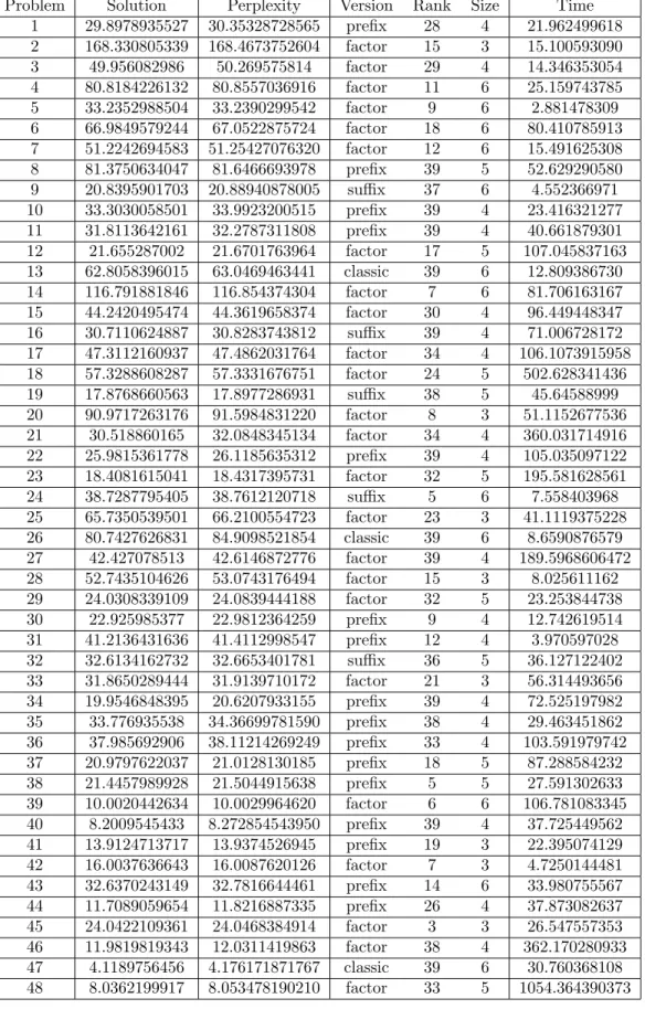
However, the results of the best run on each problem, gi-ven in Table 1 (in Annex), show that egi-ven without a smoo-thing phase the toolbox can obtain perplexity scores close to the optimal ones. This would not have permitted the winning of the competition, but it is good enough to be no-ticed. On can notice that these results are slightly different than the ones published for the first version of the toolbox, Sp2Learn [ABDE16] : in addition to small variations due to numerical instability, a bug in the prefix and suffix va-riants was fixed which allows these vava-riants to obtain better scores.
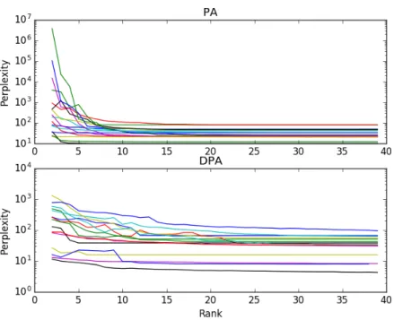
The runs realized using the toolbox also allow to eva-luate the impact of the value given to the rank parameter. Figure 2 shows the evolution of perplexity on the problems whose target machines are Probabilistic Automata (top) and Deterministic Probabilistic Automata (bottom). This curves were obtained using the classic version of the Han-kel matrix for DPA and the factor variant for PA. In both cases, values of lrows and lcolumns were set to 5.
These results show that in a first phase the perplexity can oscillate when the rank increases. However, in a second phase, the perplexity seems to decrease to a minimal va-lue and then stay stable. This second step is likely to be reached when the value of the rank parameter is equal to the rank of the target machine. At that moment, inferred singular values correspond to the target ones and adding
other values later has no impact. Indeed, if the empirical Hankel matrix was the target one, these values would be null. But even if it is not the case, which is likely in this experimental context, the results show that their values are small enough to not degrade the quality of the learning.
Figure 3 shows the average percentage on all problems of the 3-gram uses to find the probability of a test string. Re-member that this happens for strings on which the learned automata returns a non-positive weight. These percentages are given for each possible rank parameter. Each curve cor-responds to a given value of the size parameter, that is the maximal length of elements taken into account to build the Hankel matrix.
Globally, the use of 3-gram is quite rare, as less than 1.3% of strings requires its use. On the one hand, models built on large Hankel matrices tend to need less uses of 3-gram. On the other hand, models made using a large rank seem to require slightly more uses of 3-gram. This might be due to the overfitting that may occur when the rank parameter is set higher than the actual rank. Notice that no result is possible with large ranks for Hankel matrices made of too few rows and columns : as the dimensions of the matrix are smaller than the asked rank, a SVD cannot be computed.
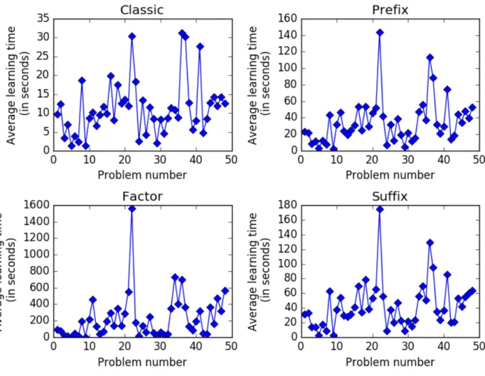
Finally, Figure 4 shows the learning time of the toolbox on the PAutomaC problems. Each point corresponds to the average computation time of all runs using a given version of the Hankel matrix, in seconds. Clearly, the classic version is the fastest while the factor one is the slowest, suffix and prefix ones are standing in a middle ground. This is expec-ted since the factor version is the less sparse of the Hankel matrix variants. Another not really surprising observation is that the behavior of the prefix and suffix versions are extremely close.
Globally, these values show that the running time of the toolbox is reasonable, even for the slowest variant : on all but one problem the factor version took less than an hour and a half on average.
5
Future developments
The version of the Scikit-SpLearn presented here is 1.1. We are currently working on extending the functionalities of the toolbox, by adding new features for instance related to :
— The word error rate (WER) is a widely used measure for the learning quality.
— Saving and loading WA has to be done efficiently. — Large automata require sparse representation. — Basis selection is a topical issue in spectral learning. We are also planning to develop new useful methods, starting with a Baum-Welch one, that would complete the learning process by allowing a real smoothing phase after the spectral learning one. We might also turn our attention to closely related and promising new algorithms, like the one of Glaude et al. [GP16].
Finally, we are also considering the development of a si-milar tool for structured inputs, such that tree and graph, as spectral methods have been proposed in this context.
R´
ef´
erences
[ABDE16] D. Arrivault, D. Benielli, F. Denis, and R. Ey-raud. Sp2Learn : A toolbox for the spectral learning of weighted automata. In Proceedings of the International Conference on Grammati-cal Inference, volume 57 of Proceedings of Ma-chine Learning Research, pages 105–119, 2016. [Bai11] R. Bailly. M´ethodes spectrales pour l’inf´erence
grammaticale probabiliste de langages stochas-tiques rationells. PhD thesis, Aix-Marseille Uni-versity, 2011.
[BBB+96] A. Beimel, F. Bergadano, N. H. Bshouty, E. Ku-shilevitz, and S. Varricchio. On the applications of multiplicity automata in learning. In 37th Annual Symposium on Foundations of Compu-ter Science, FOCS, pages 349–358, 1996. [BCLQ14] B. Balle, X. Carreras, F. Luque, and A.
Quat-toni. Spectral learning of weighted automata. Machine Learning, 96(1-2) :33–63, 2014. [BDR09] R. Bailly, F. Denis, and L. Ralaivola.
Gramma-tical inference as a principal component analysis problem. In 26th International Conference on Machine Learning, pages 33–40, 2009.
[BEL+16] B. Balle, R. Eyraud, F. M. Luque, A. Quat-toni, and S. Verwer. Results of the sequence prediction challenge (SPiCe) : a competition on learning the next symbol in a sequence. In Proceedings of the International Conference on Grammatical Inference, volume 57 of Procee-dings of Machine Learning Research, pages 132– 136, 2016.
[BHD10] R. Bailly, A. Habrard, and F. Denis. A spec-tral approach for probabilistic grammatical in-ference on trees. In Proceedings of Algorithmic Learning Theory, pages 74–88, 2010.
[BR88] J. Berstel and C. Reutenauer. Rational series and their languages. EATCS monographs on theoretical computer science. Springer-Verlag, 1988.
[CO94] R. Carrasco and J. Oncina. Learning stochas-tic regular grammars by means of a state mer-ging method. In 2nd International Colloquium on Grammatical Inference, ICGI, volume 862 of LNAI, pages 139–150. Springer-Verlag, 1994. [CT91] T. Cover and J. Thomas. Elements of
Informa-tion Theory. John Wiley and Sons, New York, NY, 1991.
[DDE05] P. Dupont, F. Denis, and Y. Esposito. Links between probabilistic automata and hidden
Figure 2 – Perplexity evolution with the rank on problems whose targets are Probabilistic Automata (top) and Deterministic Probabilistic Automata (bottom). Each line corresponds to one PAutomaC problem.
Figure 3 – Average percentage of 3-gram uses to find the probability of a test string for different values of the rank parameter (recall that the toolbox uses the trigram iff a test string is given a non-positive value by the learned WA). Each curve corresponds to a value of the maximal length of elements of the Hankel matrix.
markov models : probability distributions, lear-ning models and induction algorithms. Pattern Recognition, 38(9) :1349–1371, 2005.
[DEH06] F. Denis, Y. Esposito, and A. Habrard. Lear-ning rational stochastic languages. In 19th annual Conference on Learning Theory, pages 274–288, 2006.
[DGH16] F. Denis, M. Gybels, and A. Habrard. Dimension-free concentration bounds on hankel matrices for spectral learning. Journal of Ma-chine Learning Research, 17(31) :1–32, 2016. [GDH14] M. Gybels, F. Denis, and A. Habrard. Some
improvements of the spectral learning approach for probabilistic grammatical inference. In 12th International Conference on Grammatical Infe-rence, ICGI, pages 64–78, 2014.
[GP16] H. Glaude and O. Pietquin. PAC learning of probabilistic automaton based on the method of moments. In 33rd International Conference on Machine Learning, pages 820–829, 2016. [HKZ09] D. Hsu, S. Kakade, and T. Zhang. A spectral
al-gorithm for learning hidden markov models. In Conference on Computational Learning Theory (COLT), 2009.
[KW14] S. Kiefer and B. Wachter. Stability and Com-plexity of Minimising Probabilistic Automata, pages 268–279. 2014.
[Moh09] M. Mohri. Handbook of Weighted Automata, chapter Weighted Automata Algorithms, pages 213–254. Springer Berlin Heidelberg, 2009. [PVG+11] F. Pedregosa, G. Varoquaux, A. Gramfort,
V. Michel, B. Thirion, O. Grisel, M. Blondel, P. Prettenhofer, R. Weiss, V. Dubourg, J. Van-derplas, A. Passos, D. Cournapeau, M. Brucher, M. Perrot, and E. Duchesnay. Scikit-learn : Ma-chine learning in Python. Journal of MaMa-chine Learning Research, 12 :2825–2830, 2011. [SBG10] S. Siddiqi, B. Boots, and G. Gordon.
Reduced-rank hidden Markov models. In 13th Interna-tional Conference on Artificial Intelligence and Statistics, 2010.
[Sch61] M.P. Sch¨utzenberger. On the definition of a family of automata. Information and Control, 4(2) :245 – 270, 1961.
[TJ15] M. Thon and H. Jaeger. Links between mul-tiplicity automata, observable operator models and predictive state representations – a unified learning framework. Journal of Machine Lear-ning Research, 16 :103–147, 2015.
[VEdlH14] S. Verwer, R. Eyraud, and C. de la Higuera. PAutomaC : a probabilistic automata and hid-den markov models learning competition. Ma-chine Learning, 96(1-2) :129–154, 2014.
Annex
Problem Solution Perplexity Version Rank Size Time 1 29.8978935527 30.35328728565 prefix 28 4 21.962499618 2 168.330805339 168.4673752604 factor 15 3 15.100593090 3 49.956082986 50.269575814 factor 29 4 14.346353054 4 80.8184226132 80.8557036916 factor 11 6 25.159743785 5 33.2352988504 33.2390299542 factor 9 6 2.881478309 6 66.9849579244 67.0522875724 factor 18 6 80.410785913 7 51.2242694583 51.25427076320 factor 12 6 15.491625308 8 81.3750634047 81.6466693978 prefix 39 5 52.629290580 9 20.8395901703 20.88940878005 suffix 37 6 4.552366971 10 33.3030058501 33.9923200515 prefix 39 4 23.416321277 11 31.8113642161 32.2787311808 prefix 39 4 40.661879301 12 21.655287002 21.6701763964 factor 17 5 107.045837163 13 62.8058396015 63.0469463441 classic 39 6 12.809386730 14 116.791881846 116.854374304 factor 7 6 81.706163167 15 44.2420495474 44.3619658374 factor 30 4 96.449448347 16 30.7110624887 30.8283743812 suffix 39 4 71.006728172 17 47.3112160937 47.4862031764 factor 34 4 106.1073915958 18 57.3288608287 57.3331676751 factor 24 5 502.628341436 19 17.8768660563 17.8977286931 suffix 38 5 45.64588999 20 90.9717263176 91.5984831220 factor 8 3 51.1152677536 21 30.518860165 32.0848345134 factor 34 4 360.031714916 22 25.9815361778 26.1185635312 prefix 39 4 105.035097122 23 18.4081615041 18.4317395731 factor 32 5 195.581628561 24 38.7287795405 38.7612120718 suffix 5 6 7.558403968 25 65.7350539501 66.2100554723 factor 23 3 41.1119375228 26 80.7427626831 84.9098521854 classic 39 6 8.6590876579 27 42.427078513 42.6146872776 factor 39 4 189.5968606472 28 52.7435104626 53.0743176494 factor 15 3 8.025611162 29 24.0308339109 24.0839444188 factor 32 5 23.253844738 30 22.925985377 22.9812364259 prefix 9 4 12.742619514 31 41.2136431636 41.4112998547 prefix 12 4 3.970597028 32 32.6134162732 32.6653401781 suffix 36 5 36.127122402 33 31.8650289444 31.9139710172 factor 21 3 56.314493656 34 19.9546848395 20.6207933155 prefix 39 4 72.525197982 35 33.776935538 34.36699781590 prefix 38 4 29.463451862 36 37.985692906 38.11214269249 prefix 33 4 103.591979742 37 20.9797622037 21.0128130185 prefix 18 5 87.288584232 38 21.4457989928 21.5044915638 prefix 5 5 27.591302633 39 10.0020442634 10.0029964620 factor 6 6 106.781083345 40 8.2009545433 8.272854543950 prefix 39 4 37.725449562 41 13.9124713717 13.9374526945 prefix 19 3 22.395074129 42 16.0037636643 16.0087620126 factor 7 3 4.7250144481 43 32.6370243149 32.7816644461 prefix 14 6 33.980755567 44 11.7089059654 11.8216887335 prefix 26 4 37.873082637 45 24.0422109361 24.0468384914 factor 3 3 26.547557353 46 11.9819819343 12.0311419863 factor 38 4 362.170280933 47 4.1189756456 4.176171871767 classic 39 6 30.760368108 48 8.0362199917 8.053478190210 factor 33 5 1054.364390373
Table 1 – Best results on the PAutomaC data. Solution corresponds to the minimal perplexity (the one of the target machine) ; Perplexity is the perplexity obtained by the best run of the toolbox ; Version indicates which version of the Hankel matrix was used ; Rank gives the value of parameter rank for that run ; Size is the maximal length of elements considered for the Hankel matrix ; Time is the computation time of the run (in seconds). Problems marked with a star are the ones whose training set contains 100 000 strings (vs 20 000).