Étude d'un écoulement en circulation naturelle d'hélium diphasique en régime transitoire

HAL Id: tel-01350866

https://tel.archives-ouvertes.fr/tel-01350866

HAL is a multi-disciplinary open access archive for the deposit and dissemination of sci-entific research documents, whether they are pub-lished or not. The documents may come from teaching and research institutions in France or abroad, or from public or private research centers.

L’archive ouverte pluridisciplinaire HAL, est destinée au dépôt et à la diffusion de documents scientifiques de niveau recherche, publiés ou non, émanant des établissements d’enseignement et de recherche français ou étrangers, des laboratoires publics ou privés.

diphasique en régime transitoire

Hernan Furci

To cite this version:

Hernan Furci. Étude d’un écoulement en circulation naturelle d’hélium diphasique en régime tran-sitoire. Mechanics of the fluids [physics.class-ph]. Université Paris-Saclay, 2015. English. �NNT : 2015SACLS243�. �tel-01350866�

NNT : 2015SACLS243

THESE DE DOCTORAT

DE L’UNIVERSITE PARIS-SACLAY,

préparée

à l’Université de Paris Sud

ÉCOLE DOCTORALE N°576

Particules hadrons énergie et noyau : instrumentation, image, cosmos et simulation

Spécialité de doctorat :

Physique d’accélérateurs

Par

M. Hernán Furci

Etude d'un écoulement en circulation naturelle

d'hélium diphasique en régime transitoire

Thèse présentée et soutenue à Gif-sur-Yvette, le 13 Novembre 2015 :

Composition du Jury :

M. J. Bonjour, Professeur, INSA de Lyon, Présidente du Jury et Rapporteur M. M. Breschi, Professeur, Università di Bologna, Rapporteur

M. J. Amrit, Docteur, Maître de Conférences, Université Paris-Sud, Examinateur M. L. Bottura, Docteur, CERN, Examinateur

M. J.-L. Duchâteau, Docteur, Conseiller Scientifique, CEA de Cadarache, Examinateur M. R. van Weelderen, Docteur, CERN, Examinateur

M. B. Baudouy, Docteur HDR, CEA de Saclay, Directeur de thèse Mme. C. Meuris, Docteur, Invitée

Université Paris-Saclay Espace Technologique / Immeuble Discovery

Route de l’Orme aux Merisiers RD 128 / 91190 Saint-Aubin, France

Titre : Etude d'un écoulement en circulation naturelle d'hélium diphasique en regime transitoire Mots clés : hélium, circulation naturelle, échange thermique, transitoire, cryogénie

Résumé : Les boucles de circulation naturelle

d'hélium diphasiques sont utilisées comme systèmes de refroidissement d'aimants supraconducteurs de grande envergure, vus leurs avantages inhérents de sûreté et d'entretien. Des exemples sont le détecteur CMS au CERN (déjà en opération) ou les aimants du spectromètre R3B-GLAD au GSI (en installation). Une des préoccupations majeures lors du refroidissement par ébullition est la crise d'ébullition : la dégradation soudaine du transfert de chaleur pariétal au-delà d'une certaine valeur de flux de chaleur, dénommée critique. L'augmentation de température de paroi qui en résulte peut entrainer la perte de l'état supraconducteur de l'aimant. Les boucles de circulation naturelle à l'hélium ont déjà été étudiées expérimentalement et numériquement en régime permanent, spécialement en régimes pré-critiques (ébullition nucléée). Les travaux sur les transferts de masse et de chaleur en hélium en ébullition en régime transitoire présents dans la littérature ciblent principalement des systèmes de petites dimensions, des canaux très étroits ou trop courts, ou l'ébullition en bain. Bien que des comportements qualitativement similaires sont attendus, l'extrapolation de ces résultats à une boucle de circulation naturelle n'est pas évident, si possible. C'est pourquoi une étude particulière du comportement thermohydraulique transitoire de boucles d'hélium en circulation naturelle, lors d'une augmentation soudaine de la charge thermique, est nécessaire.

Une partie de cette étude consiste en des expériences sur une boucle d'hélium diphasique en circulation naturelle de 2 m de haut, à 4,2 K. Deux sections chauffées verticales de diamètre différent (10 et 6 mm) et d'environ 1 m de longueur ont été testées. Les transitoires sont induits par une marche soudaine de puissance. Deux types de condition initiale ont été considérés : statique (sans puissance initiale), et en équilibre dynamique (puissance initiale non-nulle). L'évolution de la température de paroi le long de la section, le débit massique et la perte de charge a été mesurée.

Parmi d'autres phénomènes, un fort intérêt a été porté au début de la crise d'ébullition. Les valeurs limites de flux de chaleur final auxquelles la crise arrive ont été déterminées. D'un côté, on a observé que la crise peut avoir lieu de façon temporaire ou permanente à une puissance appréciablement plus faible qu'en régime permanent. De l'autre côté, l'augmentation de la circulation initiale, à travers le flux de chaleur initial, peut inhiber partiellement ou totalement cette crise d'ébullition prématurée. On a déterminé que cette dégradation du transfert de chaleur est le résultat de deux phénomènes en compétition, véritablement inhérents à la circulation naturelle : une étape initiale d'accumulation uniforme de vapeur, avec inversion ou diminution de la vitesse d'entrée, et l'établissement ultérieur de la circulation, avec le transit d'un front froid depuis l'entrée. Une analyse semi-empirique nous a permis de déterminer un critère, basé sur l'évolution dynamique du profil spatial du titre massique, pour prédire le déclenchement de la crise. Néanmoins, il est nécessaire de connaître à priori l'évolution du débit massique pour pouvoir appliquer ce critère.

La dernière partie de ce travail est dévouée à la production et validation de modèles et outils de calcul pour la simulation du comportement thermohydraulique d'un tel système. Deux options de modélisation sont présentées. L'une est une simplification des équations du modèle homogène 1D des écoulements diphasiques (mise en place en COMSOL) ; l'autre reprend le modèle homogène tel quel (programmé en C). Les simulations d'évolution du débit massique sont en assez bon accord avec les mesures, à l'exception d'un léger déphasage temporel. Ceci pourrait être dû à la combinaison d'un retard de l'instrumentation pour la mesure du débit et de l'inexactitude des hypothèses de base du modèle homogène lors de transitoires très violents.

Université Paris-Saclay Espace Technologique / Immeuble Discovery

Route de l’Orme aux Merisiers RD 128 / 91190 Saint-Aubin, France

Title : Study of two-phase boiling helium natural circulation loops in transient regime Keywords : helium, natural circulation, heat transfer, transient, cryogenics

Abstract : Boiling helium natural circulation

loops are used as the cooling system of large superconducting magnets because of their inherent safety and maintenance advantages. Examples are the cooling systems of the CMS detector solenoid magnet at CERN (already in operation) or the R3B-GLAD spectrometer magnet at GSI (in installation phase). A major concern in boiling cooling systems is that of boiling crisis: a sudden deterioration of the wall heat transfer takes place when the surface heat flux exceeds a certain value, called the critical heat flux (CHF). The resulting high temperatures on the wall could ultimately entail the loss of superconducting state of the magnet.

Helium natural circulation loops have already been studied experimentally and numerically in steady state, especially in the pre-critical heat and mass transfer regimes (nucleate boiling). Works on transient boiling heat and mass transfer in helium present in the literature are mostly focused on small systems, very narrow channels, too short pipes or pool boiling. Although it is expected to find qualitative similarities with already observed behavior, the extrapolation to a natural circulation loop is not easy, if even possible. Hence the need for a particular study on the transient thermohydraulic behavior of helium natural circulation loops, after sudden increases in the heat load of the circuit.

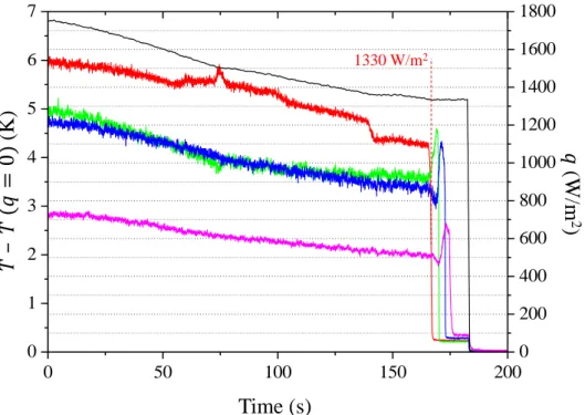
A part of this study consists of experiments conducted in a 2-meter high two-phase helium natural circulation loop at 4.2 K temperature. Two vertical heated sections with different diameters (10 and 6 mm) and around 1 m length were tested. Heat load transients were driven by a step-pulsed heat load. Transients with two types of initial conditions have been studied: static loop (no initial power applied) and in-dynamic-equilibrium loop (non-zero initial power applied). The evolutions of wall temperature along the heated section, total mass flow rate and pressure drop were measured.

Among other phenomena, the nature of the onset of boiling crisis has received a special attention. The values of final heat flux limits for its occurrence have been determined. On the one hand, we observed that boiling crisis can take place in temporary or stable fashion at power significantly lower than in steady state. On the other hand, the increase of initial circulation, by raising initial heat flux, can inhibit partially or completely this power-premature boiling crisis. We could determine that this heat transfer deterioration is the result of two competing phenomena, veritably inherent to the natural circulation feature of the system: an initial stage of uniform vapor accumulation with inlet back-flow or velocity reduction, and the ulterior onset of circulation with the transit of a cold front from the entrance. A semi-empirical analysis of data allowed determining a criterion, based on the dynamic evolution of the quality profile in the section, to predict the incipience of boiling crisis. It became evident that it is necessary to know how the mass flow rate of the system is going to evolve, in order to apply the mentioned criterion.

Hence, the other part of this work is aimed to the production and validation of models and calculation tools in order to simulate the thermohydraulic behavior of a two-phase helium natural circulation loop. Two modeling options are proposed. One of them consists of a simplification of the 1D two-phase homogeneous model equations (implemented in COMSOL) and the other of their full version (coded in C language). The simulated mass flow rate represents reasonably well the measured evolution except for a relatively small time phase-shift. This could be due to a combination of the delay of flow-metering instrumentation with the inaccuracy of the basic homogeneous model assumptions during violent transients.

A mis padres, Lidia y Franco,

por haberme ense˜nado a leer o las fases de la luna

Avant-propos

Cet ouvrage est le fruit de trois ans de travail de recherche. Heureusement, je n’ai pas parcouru ce chemin en solitude. Ces quelques lignes ont le but de remercier les personnes qui m’ont accompagn´e et qui ont contribu´e `a ce que cette p´eriode se d´eroule de la meilleure fa¸con possible.

Les activit´es dont ce document est le r´esultat ont ´et´e r´ealis´ees au Commissariat `a l’Energie Atomique et aux Energies Alternatives (CEA) `a Saclay, au sein du Laboratoire de Cryog´enie et Station d’Essais (LCSE) du Service d’Acc´el´erateurs, Cryog´enie et Magn´etisme (SACM) de l’Institut de Recherche sur les Lois Fondamentales de l’Univers (IRFU), dans la Division de Sciences de la Mati`ere (DSM).

Dans ce cadre, je veux commencer par remercier le CEA pour avoir enti`erement financ´e mes travaux. Je tiens aussi `a remercier la direction du SACM et du LCSE, Mess. Antoine Da¨el, Philippe Chesny, Pierre Vedrine, Philippe Bredy, Olivier Napoly, Christophe Mayri et Madame Roser Vallcorba: je les remercie pour l’accueil chaleureux dans leurs ´equipes et de leur attention pour que toutes les ressources humaines, mat´erielles et techniques soient disponibles. Merci aussi d’avoir rendu possible financi`erement ma participation `a des conf´erences et des workshops internationaux qui m’ont permis de d´ecouvrir et m’int´egrer `a cette communaut´e de la cryog´enie et des aimants supraconducteurs.

Au sein du LCSE, je veux remercier Mess. Michel Sueur et Gilles Authelet d’avoir ´et´e tr`es disponibles pour livrer une des ressources fondamentales pour mes travaux, l’h´elium, et d’avoir fait tout ce qui ´etait possible mˆeme quand je le commandais avec peu d’anticipation.

Je tiens aussi `a remercier les personnes qui ont travaill´e plus directement avec moi le long de ces trois ans.

En premier lieu, je dois mentionner Mme. Chantal Meuris, qui ´etait initialement la directrice de ce travail. Nos r´eunions d’avancement et discussions plus informelles ont ´et´e tr`es utiles pour orienter et cadrer ma recherche, grˆace `a son regard tr`es exp´eriment´e depuis un angle beaucoup plus large.

Ensuite, je veux remercier de leur apport Mess. Guillaume Meyer et Vincent Balssa, qui ont travaill´e avec moi en tant que stagiaires. Les encadrer a ´et´e une exp´erience enrichissante et j’ai beaucoup appr´eci´e la fa¸con dans laquelle leurs questions ont apport´e de l’air frais `a mes analyses. Pour la r´ealisation des exp´eriences j’ai compt´e avec l’aide de Mess. Antoine Bonelli et Aur´elien Four. Je remercie Antoine pour quelques petits conseils pour souder des tous petits fils et pour avoir pr´epar´e un ensemble des capteurs de temp´erature dont je me suis servi. Je remercie Aur´elien pour m’avoir transmis avec beaucoup de patience et p´edagogie une ´enorme quantit´e de savoir-faire technique, sp´ecialement au tout d´ebut de ce travail, et pour m’avoir offert un support indispensable lors de toutes les campagnes exp´erimentales.

Si ce travail a ´et´e tr`es fructueux, c’est en grande mesure grˆace `a M. Bertrand Baudouy, mon directeur de th`ese. Je le remercie de sa pr´esence constante, de sa g´en´erosit´e, de son humour et de sa sympathie, juste pour mentionner quelques-unes de ses qualit´es humaines. Je veux lui exprimer ma reconnaissance non seulement pour son professionnalisme et son vaste savoir du domaine, mais aussi pour sa franchise, sa critique, ses paroles d’encouragement et ses conseils (techniques ou pas) le long de ces trois ans. C’est un vrai honneur qu’il m’ait confi´e la r´ealisation de ce projet et qu’il ait ´et´e le premier lecteur de tous les ´ecrits qui en ont r´esult´e.

Je me sens tr`es honor´e d’avoir compt´e avec la pr´esence de Mess. Jocelyn Bonjour, Marco Breschi, Luca Bottura, Rob van Weelderen, Jay Amrit et Jean-Luc Duchˆateau dans mon jury de th`ese. Je les remercie de l’int´erˆet qu’ils ont prˆet´e `a mon sujet et d’avoir contribu´e `a la qualit´e de

lors de la soutenance.

Cette p´eriode n’aurait pas ´et´e pareille sans les nombreuses personnes que, sans ˆetre impliqu´ees dans mon travail, j’ai cˆotoy´ees au sein du SACM. J’adresse un merci sp´ecial `a tous ceux avec qui j’ai partag´e des innombrables d´ejeuners et pauses caf´e, pour les discussions sur tout et n’importe quoi et les moments de bonne humeur.

En dernier, je veux exprimer ma gratitude `a toutes ces personnes qui font partie de ma vie personnelle et qui m’ont soutenu le long de mon doctorat, et mˆeme depuis toujours. Pour les petits et grands gestes, pour me corriger le fran¸cais, pour me faire `a manger quand j’avais peu de temps, pour l’encouragement, pour l’´ecoute, pour les conseils... Mais surtout, pour les rires, pour les moments de joie et de c´el´ebration.

Contents

1.2.2 The transition from normal to superconducting . . . 6

1.2.3 Superconducting magnets materials . . . 7

1.2.4 Superconducting magnets cables . . . 8

1.3 Magnet cooling techniques . . . 9

1.4 Superconducting magnets cooled by natural circulation . . . 11

1.4.1 The superconducting solenoid for the CMS detector . . . 11

1.4.2 The GLAD superconducting spectrometer for R3B . . . 13

Final comments . . . 16

2 Physical background 17 2.1 Boiling heat transfer . . . 17

2.1.1 Pool boiling regimes . . . 17

2.1.2 Forced convective boiling regimes . . . 20

2.1.3 Boiling crisis prediction in channel flow . . . 21

2.1.4 Heat transfer in the nucleate boiling regime . . . 24

2.2 Two-phase flow modeling . . . 28

2.2.1 Basic definitions and conservation equations . . . 29

2.2.2 The homogeneous two-phase flow model . . . 31

2.3 The natural circulation principle . . . 33

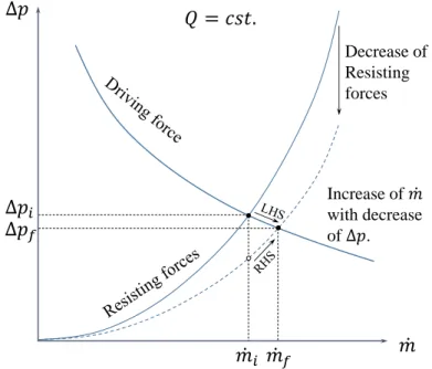
2.3.1 Dynamics of a natural circulation loop . . . 33

2.3.2 Two-phase loop equilibrium . . . 34

2.4 Helium flows . . . 37

2.4.1 Phase diagram . . . 37

2.4.2 Physical properties at saturation . . . 38

2.4.3 Flow Patterns . . . 39

2.4.4 Void fraction . . . 40

2.4.5 Review on two-phase friction estimation . . . 41

2.5.1 The findings of pool boiling experiments . . . 44

2.5.2 Transient boiling in channels . . . 46

2.6 The contribution of this work . . . 48

3 The experimental facility 51 3.1 The cryostat . . . 51

3.2 The insert . . . 53

3.3 The elements of the loop . . . 54

3.4 Heating configurations . . . 56

3.5 Instrumentation and measurements techniques . . . 56

3.5.1 Wall temperature . . . 57

3.5.2 Mass flow rate . . . 61

3.5.3 Pressure drop . . . 62

3.5.4 Power supply and measurement . . . 63

3.5.5 Other Instrumentation . . . 64

3.6 Signal data acquisition . . . 66

3.7 Preparation of the experiment . . . 68

3.7.1 Check-up actions . . . 68

3.7.2 Start up actions . . . 69

Final comments . . . 69

4 Study of the onset and hysteresis of boiling crisis in steady state 71 4.1 Realization of experiments . . . 71

4.1.1 Experimental protocol . . . 71

4.1.2 Data treatment . . . 72

4.1.3 Measured evolution of thermohydraulic variables . . . 73

4.2 Determination and characterization of flow boiling regimes . . . 73

4.2.1 Experimental observations on boiling crisis onset . . . 73

4.2.2 Prediction of the critical heat flux . . . 78

4.2.3 Description of post-CHF heat transfer features . . . 80

4.2.4 Observations on rewetting during the decreasing power experiment . . . . 83

4.3 Study of the hydraulic effects of boiling crisis . . . 85

4.3.1 Experimental observations on pressure drop and mass flow rate during crisis development . . . 86

4.3.2 Evaluation of pressure drop prediction methods during boiling crisis . . . 87

4.3.3 Creation of a new film boiling pressure drop prediction model . . . 91

Summary . . . 95

5 Study of stepwise heat load induced transients with static initial condition 97 5.1 Realization of experiments . . . 97

5.1.1 Experimental protocol . . . 98

5.1.2 Measured time evolution overview . . . 99

5.2 Characterization of the initiation of the transient . . . 99

5.2.1 Study of the effect of heat flux on time evolution . . . 99

5.2.2 Characterization of the mass flow rate evolution . . . 104

5.2.3 Characterization of heat transfer during the initiation of boiling . . . 108

5.3 Characterization of boiling crisis during transients . . . 113

5.3.1 Determination of transient critical heat flux . . . 114

5.3.2 Identification of interesting time response parameters of transient boiling crisis . . . 115

5.3.3 Data treatment for critical transients . . . 115 5.3.4 Comparison of transient to quasi-steady temperatures in post-CHF regimes117

Contents

5.3.5 Determination of the dependence of critical time on heat flux . . . 120

5.4 Study of transient boiling crisis initiation regimes . . . 123

5.4.1 The linear regime . . . 124

5.4.2 Comparison of critical time data with models . . . 126

5.4.3 Study of incipience of the linear-regime . . . 129

5.4.4 The quadratic regime . . . 131

5.4.5 The high-tc regime . . . 133

Summary . . . 134

6 Study of the effect of a dynamic equilibrium initial condition on stepwise heat load induced transients 137 6.1 Realization of experiments . . . 137

6.1.1 Experimental protocol . . . 137

6.1.2 Measured time evolution . . . 138

6.1.3 Identification of main effects of initial conditions on transients . . . 144

6.2 Experimental determination of behavior boundaries . . . 145

6.2.1 Determination of the inhibition heat flux . . . 146

6.2.2 Identification of transition between crisis initiation regimes . . . 146

6.2.3 Identification of the link between the transition regimes and the inhibition of crisis . . . 146

6.2.4 Drawing the experimental behavior maps . . . 150

6.3 Theoretical study of the system with arbitrary initial condition . . . 151

6.3.1 Simplifying Assumptions . . . 151

6.3.2 The equations . . . 151

6.3.3 Numerical approach . . . 153

6.3.4 Observation of the effect of initial condition on quality evolution . . . 153

6.4 Determination of a criterion for boiling crisis initiation . . . 155

Summary . . . 158

7 Modeling of the boiling helium loop in transient regime 161 7.1 Representation of the loop in 1D . . . 161

7.2 Development of a simplified model . . . 162

7.2.1 Simplification of the equations . . . 162

7.2.2 The resulting simplified model . . . 168

7.3 Implementation of the simplified model in COMSOL . . . 171

7.3.1 Description of the environment . . . 172

7.3.2 Solving strategy . . . 172

7.3.3 Comparison of the simplified model simulations to the experimental data 174 7.4 Solution of the non-simplified model . . . 175

7.4.1 Structure of the program . . . 175

7.4.2 Input parameters . . . 178

7.4.3 Numerical method . . . 179

7.4.4 Fluid properties . . . 181

7.4.5 Initial conditions . . . 181

7.4.6 Boundary conditions . . . 182

7.4.7 Comparison of simulated and measured evolutions . . . 185

7.5 Evaluation of the transition to boiling crisis criteria with the simulators . . . 186

Summary . . . 186

Synthesis and comments 189

Appendix A R´esum´e substantiel en fran¸cais 195

A.1 Introduction . . . 195

A.2 Montage exp´erimental . . . 196

A.3 D´emarche exp´erimentale . . . 198

A.4 Comportement de la crise d’´ebullition en r´egime permanent . . . 198

A.4.1 Le d´ebut et d´eveloppement de la crise d’´ebullitiion . . . 198

A.4.2 Les effets hydrauliques de la crise d’´ebullition . . . 199

A.5 Transitoires avec condition initiale statique . . . 200

A.5.1 La r´eponse hydraulique . . . 200

A.5.2 Les r´egimes de transfert de chaleur . . . 201

A.6 Transitoires avec condition initiale dynamique . . . 203

A.6.1 R´esum´e des principaux effets observ´es . . . 203

A.6.2 Carte de comportements . . . 204

A.6.3 Un crit`ere empirique pour l’arriv´ee de la crise . . . 204

A.7 Mod´elisation de l’´ecoulement diphasique . . . 205

A.7.1 Un mod`ele simplifi´e . . . 205

A.7.2 Le mod`ele non-simplifi´e . . . 205

A.7.3 Validation et limitations des simulations num´eriques . . . 205

A.8 Conclusions . . . 206

Appendix B The film boiling friction model equations 209 Appendix C Demonstrations concerning loop dynamics modeling 211 C.1 Simplified velocity profile . . . 211

C.2 Alternative approach for the integral momentum equation . . . 212

C.3 Cross section changes . . . 213

List of publications I

References III

List of Figures

1.1 Critical surface of a superconductor. . . 7

1.2 Critical characteristics of some superconductors. . . 8

1.3 Cross section of a Rutherford cable. . . 9

1.4 Cross-sectional view of ITER conductors . . . 10

1.5 The CMS magnet. . . 12

1.6 CMS cooling system. . . 14

1.7 Illustration of the R3B-GLAD systems. . . 15

2.1 Pool boiling curve. . . 18

2.2 Pool boiling regimes . . . 19

2.3 Forced convective boiling regimes. . . 22

2.4 Bubble nucleation in a cavity . . . 25

2.5 Nucleate boiling cycle. . . 27

2.6 Nucleate boiling heat transfer mechanisms. . . 29

2.7 One-dimensional two-phase natural circulation loop . . . 33

2.8 Response of the equilibrium point to the overall friction coefficient change in a natural circulation loop. . . 36

2.9 Helium phase diagram . . . 37

2.10 Two-phase flow pattern chart for helium in vertical channels . . . 40

2.11 Void fraction in helium flow . . . 41

2.12 Two-phase friction factor in helium for vertical tubes . . . 42

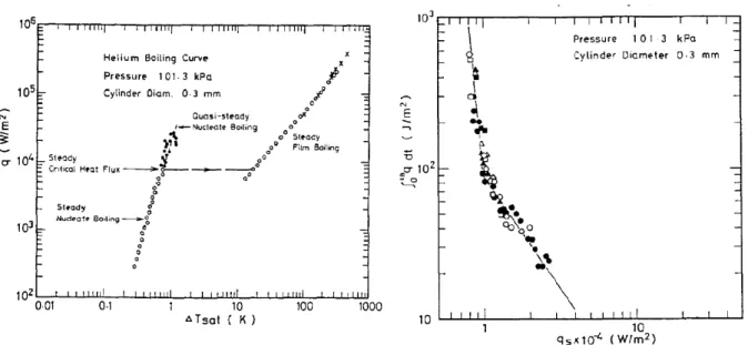
2.13 Typical temperature evolutions during transients in pool boiling in a helium bath 44 2.14 Temperature evolutions showing the homogeneous nucleation limit . . . 45

2.15 Results on nature and duration of quasi-steady nucleate boiling . . . 46

3.1 The experimental facility: (left) the insert and (right) the cryostat. . . 52

3.2 The loop elements and its intrumentation. . . 55

3.3 Diagram of a thermoresistor transducer . . . 57

3.4 Cernox sensors used for wall temperature measurements . . . 59

3.5 Dimensions of Cernox temperature transducers . . . 59

3.6 The support for AA sensors. . . 60

3.7 Working principle of a DP10 transducer. . . 63

3.8 The heating power controle and measurement technique. . . 64

3.9 Liquid level monitors. . . 65

3.10 Typical Labview Screen. . . 67

3.11 Start up of an experiment . . . 68

4.1 Power evolution during a steady state experiment. . . 72

4.2 Thermal behavior of the heated sections for steady power . . . 74

4.3 Total mass flow rate evolution for steady power . . . 75

4.5 Katto’s criteria for the CHF transition type . . . 79

4.6 Heat transfer coefficient evolution for steady power. . . 81

4.7 Temperature evolutions in transition from post-CHF to NB regime. . . 84

4.8 Schematic observed crisis evolution during rewetting experiments . . . 85

4.9 Pressure drop prediction . . . 88

4.10 Friction pressure drop prediction . . . 89

4.11 Schematic velocity profile assumed for the FB model study. . . 91

5.1 Schematic heat flux evolution in static initial condition experiments. . . 98

5.2 Time evolution in static initial condition transients at different values of qf (part 1). . . 100

5.3 Time evolution in static initial condition transients at different values of qf (part 2). . . 101

5.4 Time evolution in static initial condition transients at different values of qf (part 3). . . 102

5.5 Time evolution in static initial condition transients at different values of qf (part 4). . . 103

5.6 Transient maximum and final mass flow rate values as a function of q. . . 105

5.7 Quantitative analysis of the instantaneous hydraulic response. . . 105

5.8 Determination of the end of the pure conduction phase. . . 111

5.9 Global temperature values during stepwise power transients. . . 112

5.10 Parameters characterizing transient boiling crisis . . . 116

5.11 Temperature maximum and final values compared to quasi-steady state, V10. . . 118

5.12 Temperature maximum and final values compared to quasi-steady state, V06. . . 119

5.13 Simultaneous temperature evolutions for V06. . . 121

5.14 Critical time vs. final wall heat flux. . . 122

5.15 Critical time as a function of volume-averaged power. . . 125

5.16 Spatial dependence of tc× qv. . . 126

5.17 Critical product tc× qv vs. final volume specific power. . . 128

5.18 Evaluation of the transient boiling crisis incipience criterion in the linear regime by the ‘uniform expansion-transit time’ model . . . 132

6.1 Schematic heat flux evolution in non-static initial condition experiments. . . 138

6.2 The effect of initial heat flux on time evolution (Part 1) . . . 139

6.3 The effect of initial heat flux on time evolution (Part 2) . . . 140

6.4 The effect of initial heat flux on time evolution (Part 3) . . . 141

6.5 The effect of initial heat flux on time evolution (Part 4) . . . 142

6.6 The effect of initial heat flux on time evolution (Part 5) . . . 143

6.7 The effect of initial heat flux on time evolution (Part 6) . . . 143

6.8 Criterion for finding the crisis inhibition heat flux . . . 147

6.9 Effect of qf on qinh . . . 147

6.10 The effect of initial heat flux on critical time in V10 . . . 148

6.11 The effect of initial heat flux on critical time in V10 — linear regime life at a given position as a function of qi and qf . . . 148

6.12 The effect of initial heat flux on critical time in V06 . . . 149

6.13 The effect of initial heat flux on critical time in V06 — linear regime life at a given position as a function of qi and qf . . . 149

6.14 Experimental boiling crisis transient behavior maps . . . 152

6.15 Alternative types of behavior maps . . . 153

6.16 Simulation of thermodynamic quality for non-static initial condition . . . 154

List of Figures

7.1 Transformation of the loop into a 1D domain. . . 163

7.2 Comparison of simplified model simulations to experiments. . . 176

7.3 Simulated time evolution of property profiles with the simplified model. . . 177

7.4 Comparison of simulations with the two models to experiments. . . 184

7.5 Quality-based incipient cases analysis using the developed models. . . 186

7.6 Quality-based incipient cases analysis: comparison with experiments. . . 187

List of Tables

2.1 Saturation properties of water, nitrogen and helium. . . 38

3.1 Heating section parameters . . . 56

4.1 CHF and RHF values found experimentally . . . 77

4.2 Values of CHF predicted by Katto’s correlation . . . 79

5.1 Transient critical heat flux, qc,tand qc,p . . . 115

5.2 Values of the product tc× qv . . . 124

5.3 Transit time and quality analysis applied to incipient linear regime boiling crisis cases . . . 131 6.1 Quality analysis of linear boundary cases for transients with qi ̸= 0, section V06. 156

Nomenclature

Roman letters

A cross section area m2

Bc superconductor critical magnetic field T

B FB model parameter m3/7 s−3/7

˜

B non-dimensional FB model parameter = B

V_h3/7

C specific heat J kg−1 K−1

D diameter m

e specific internal energy J kg−1

f friction factor

G mass flux kg m−2 s−1

H Momentum integral: ∫ρu ds kg m−1 s−1

h specific enthalpy J kg−1

hlg vaporization latent heat J kg−1

I electric current A

Jc superconductor critical current density A m−2

k thermal conductivity W m−1 K−1

L tube length m

9

m mass flow rate kg s−1

P pressure Pa

p pressure Pa

q heat flux W/m2

qv = 4q_D, heat generation rate per unit volume W m−3

R electric resistance Ω

R radius m

r radial position variable m

s loop curvilinear coordinate m

∆T wall superheat: Tw− Tl K

t time s

Tc superconductor critical temperature K

U electric tension V

u velocity m s−1

V velocity m s−1

v specific volume m3 kg−1

x quality

Greek letters

α thermal diffusivity m2 s−1

α void fraction

δ film thickness m s−1

γ diffusion coefficient m2 s−1

κ Von K´arm´an constant = 0.41

µ viscosity kg m−1 s−1

Ω two-phase expansion rate: vlgqv

hlg s −1 ρ density kg m−3 σ surface tension N m−1 τ shear stress N m−2 τ transit time s

Indexes and accents

1ϕ one-phase

2ϕ two-phase

acc fluid acceleration contribution

c critical

d at bubble departure

d down-comer

d duration

e adiabatic entrance of the ascending branch

ef f effective

f at the film-liquid interface

f final

f r friction contribution

g saturated vapor

g when index of ∆p only, gravitational contribution

h heated section

h homogeneous bulk

i initial

cs current sharing

l saturated liquid

lg difference between liquid and vapor

n iteration step

p permanent crisis

r adiabatic riser

s quasi-steady state

sat saturation

sing concentrated head loss singularity

Nomenclature

t temporary crisis

u horizontal section of the U-shaped loop

w at the wall

Physical constants

Acronyms

DFFB dispersed flow film boiling DNB departure from nucleate boiling FB film boiling

HEM homogeneous equilibrium model IAFB inverted annular film boiling i.d. inner diameter

LHS left hand side

ODE ordinary differential equation PDE partial differential equation RHF rewetting heat flux

RHS right hand side SBC stable boiling crisis SNB stable nucleate boiling TBC temporary boiling crisis

Introduction

Cryogenics is today indispensable for the realization and operation of superconducting magnets, given that low temperature is required for the materials to reach the superconducting state. One option for the cooling system of superconducting magnets is that of a boiling helium natural circulation loop. In most of the cases, these systems are operated in steady state, i.e. with a time-independent heat load. Nevertheless, in some cases, a time-dependent heat load may be exerted on the system, either for operational reasons or in the case of undesired incidents. The system produces a transient response to such solicitations, a response which is not always well known. This arises the question of whether the cooling system is capable of keeping the superconductor within the temperature requirement when reacting to these external excitations. The passage of the material to the resistive state is highly undesired during the operation of a magnet, given that this could conduct to brutal energy deposition on the assembly and brutal mechanical solicitation.

Boiling helium two-phase natural circulation loops have been studied by Baudouy and Benkheira at CEA Saclay [5, 6, 8, 9]. These authors have conducted experiments in which they control the power applied on the heated section of such a system in steady state. They have tested different types of tubes as heated section, with different diameters and orientations. Their observations have allowed a very complete characterization of heat and mass transfer in the nucleate boiling regime. They have also shown that it is possible to reach boiling crisis on the heated section wall using their apparatus. Nonetheless, they have not conducted experiments with time-varying heat loads.

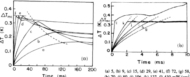
There are a few works on transient boiling heat transfer in helium or other cryogens in response to time-varying heat load in the literature [43, 63, 67, 71]. Most of these works are focused on the problem of a filament or flat surface immersed in a liquid helium pool, on which power is applied electrically. These experiments have provided very valuable results, especially for the characterization of the different heat transfer regimes that follow a sudden power injection on the heater. In particular, the work by Sinha [68] has proved that, in the case of nitrogen pool boiling around a filament, there can be a significant difference of the boiling crisis power limits in steady state or transient regime, being lower for the latter. However, not all the findings of pool boiling experiments can be extrapolated to internal flow, and in all cases, these works are focused on extremely small systems (never exceeding a few cm of length).

The problem of transient heat transfer in helium channel flow has been tackled by a few authors. Yarmak studied the case of forced flow in very narrow channels [77] and Schmidt [64], and Babitch and Pavlov [4] inside a tube immersed in a pool (flow taking place by natural circulation). These experiments were conducted in tubes shorter than 25 cm and with an internal diameter smaller than 3 mm. These studies highlight a number of phenomena that can take place during transient boiling in channels, with a particular focus on the transition to boiling crisis in unsteady conditions. They point out that transient boiling crisis can happen temporarily at lower heat flux than in steady state. They also point out the existence of a meta-stable nucleate boiling phase before the arrival of boiling crisis and they show that its duration is a function of

the power applied, different from that in pool boiling. Pavlov and Babitch, in particular, attribute this different behavior to the confinement in the channel and propose a model to predict the critical time [61]. Nevertheless, not only these systems are too small compared to the dimensions typical of magnet cooling systems, but also these experiments are not veritably conducted in a circulation loop, the mass flow rate evolution in the heated section is unknown and unstudied and, yet, the boiling crisis incipience heat flux during transients (possibly lower than that in steady state) is not thoroughly discussed and remains unpredictable.

To summarize, large helium natural circulation loops have been studied thoroughly only in steady state and mostly in pre-critical boiling regimes. The literature reveals that in wall boiling cooled systems the critical heat flux limit can be appreciably reduced in the case of violent power injections. However, the studies are restricted to systems in pool boiling or flow in very small channels, with no information on mass flow rate evolution.

For these reasons we saw the need of characterizing the dynamic behavior of a relatively large boiling helium natural circulation loop in transient regime induced by stepwise increase of wall heat flux, which is the objective of the present work.

In chapter 1 we present in more detail the role of cryogenics in the superconducting magnets field and present applications of helium natural circulation loops. In chapter 2 the physical background of phenomena associated to natural circulation loops and boiling is presented. These two chapters will provide the motivation and context for the research presented in this document. As we will see in the following paragraphs, this work is composed of two parts. The first one consist of an experimental study on a cryogenic loop, and the second one of the modeling and simulation this type of system. The elements of the experimental facility, as well as the instrumentation and the operational procedure are exposed in detail in chapter 3.

Our study starts with the experimental characterization of boiling crisis onset in a helium natural circulation loop with a heated section of more than 5 mm of inner diameter. This was done to know to what extent a link exists between steady state and transient boiling crisis and because available tools for the prediction of boiling crisis are poorly based on helium data, not to mention the anomalies that can take place concerning critical heat flux (CHF) in vertical chan-nels. To do this, we conducted experiments on such a loop with vertical heated sections of 6 and 10 mm i.d. and around 1 m long, dimensions that are representative of the tubes used in magnet cooling. In order to observe the dependence of the most significant thermohydraulic variables on heat flux and to identify the transition to boiling crisis and back to nucleate boiling, increasing and decreasing power progressions were applied on the loop. Heat flux was varied sufficiently slowly, so as to avoid the excitation of transient modes. Simultaneously, wall temperature, mass flow rate and test section pressure drop were measured. On the other hand, we calculated the critical heat flux and pressure drop predicted by the literature in our experimental conditions. We compared our experimental values to these predictions, and we have detected anomalies that can take place in these systems during and after the onset of boiling crisis. A model was conceived and evaluated to improve the prediction of pressure drop in the film boiling regime. All these actions constitute chapter 4.

Our next step was the characterization of transients induced by a stepwise power increase from a static initial condition. This would give us the limit case of the most violent possible solicitation that can be exerted on the system. For this study, we conducted experiments on the same loop, in which power is suddenly increased from zero to a final constant value. The aim was to identify the influence of this parameter on the evolution of mass flow rate and wall tem-perature, with a particular focus on the boiling crisis transition. Given the great amount of data, automatic data treatment tools were developed. These tools had to be capable of determining the occurrence of crisis and of calculating the characteristic time parameters of both mass flow rate and temperature evolutions. This tool was applied to the data in order to characterize the

Introduction influence of heat flux on these parameters, in particular on critical time, i.e. the duration of the meta-stable nucleate boiling stage before boiling crisis. The critical time that can be predicted from previous work in the literature was evaluated and compared to the experimental data. Different mechanisms for the initiation of boiling crisis were identified and described. In order to give an answer to the question of transient boiling crisis incipience heat flux and suspecting that this could be strongly linked to the evolution of natural circulation, the evolution of thermo-hydraulics in the heated section was modeled and simulated (using as input experimental inlet velocity data) for the incipient cases. These actions are presented in chapter 5.

In order to tackle the more realistic, intermediate situation in which a stepwise heat load increase comes up during the normal operation of the loop at non-nul power, another set of experiments was conducted. In these experiments the system is initially in dynamic equilibrium at a given initial heat flux and power is increased to a final value. In order to identify the influence of the initial condition on the transient, series of experiments are defined by a fixed value of final heat flux, and the initial heat flux is a varying parameter. In general, the final heat flux is chosen so as to have boiling crisis when the initial condition is static; this, with the aim of observing the effect of initial conditions on transient boiling crisis. The critical time of every single case was determined whenever crisis was observed. Its dependence on initial heat flux was systematically studied. By observing the evolution of critical time with initial and final heat flux, we determined quantitative and qualitative effects of the initial condition on the mechanism for transient boiling crisis onset. This allowed defining transient behavior charts on the initial-final heat flux plane. Still with the same hypothesis, that boiling crisis initiation in some of the regimes is governed by the thermohydraulic evolution on the heated section, the model developed before was extended to the case with a dynamic initial condition and applied to the experimental cases near the incipience boundary. The study of time evolution of local vapor fraction was used to define a criterion for boiling crisis incipience during transients. Chapter 6 presents this part of the study.

Having appreciated the importance of the evolution of the thermohydraulic variables on the onset of boiling crisis, it is desirable for future analysis to have validated models and numerical tools for their prediction, without the need of performing new experiments. With this aim, modeling options for boiling helium natural circulation loops were studied. Given the values of helium properties and previous experimental knowledge of helium flows, we found appropriate to take as a departure point the time-dependent homogeneous equilibrium model (HEM). The first approach was the analytical study of the equations with the objective of simplifying them, in order to represent the first order phenomena. Pressure effects were expected to be negligible in systems of our dimensions; neglecting them allowed us to pass from a system with three partial differential equations (PDE), to one with only one PDE and one ordinary differential equation (ODE). The obtained system was implemented in a commercial multi-physics simulation software and the simulated evolution of hydraulic behavior was compared to that measured. In order to verify certain time response discrepancies between model and experiment were due to the pressure effects simplification hypothesis, we decided to solve the full version of the equations of the HEM. To do this, we fully developed a numerical method based on finite differences and a C language code. The differences in behavior due to pressure effects were studied in order to decide if they originate the aforementioned discrepancies. The ability of this type of models to represent boiling helium natural circulation loops and predict boiling crisis was analyzed. All the work related to modeling constitutes chapter 7.

Finally, the last part of this document recapitulates the findings of this work and points out new problems to be addressed.

Chapter 1

Technological context

1.1

Cryogenics

The word cryogenics generally refers to the science and technology of producing a low temper-ature environment for applications as well as the study of materials, fluids, heat transfer and all other physical phenomena taking place at low-temperature environments. Cryogenics tem-perature range of interest is generally accepted to be below 120 K approximately, being this the temperature at which the called permanent gases (O2, N2, Ar and methane) are cold enough to

be liquified.

Applications of cryogenics are present in a wide variety of technical fields including advanced energy production and storage technologies, transportation and space programs, and a wide variety of physics and engineering research efforts. The field is very interdisciplinary consisting of essentially all the scientific community focused on low temperature technology.

One of these fields where cryogenics plays a key role is superconductivity and superconducting magnets, which constitutes the motivation of this work. In the next section we expose the implications of our research in this field.

1.2

Superconductivity

Superconductivity is the property of a material by which it is capable of conducting an electrical

current without dissipating heat by Joules effect; i.e. we say a material is superconductor when at a given condition its electrical resistance vanishes. A material with this property is called

superconductor.

Immediately, we can see the advantage of superconductors compared to normal conductors, such as copper or aluminum. In applications where huge amounts of electric current (or current density) may be required, the use of superconducting cables may reduce dramatically the cost of operation of the technological device, as less electric power will be required. On the other hand, efforts will be necessary to cool the superconductors, since superconductivity is achieved only

below a certain temperature.

1.2.1 A brief history

The discovery of superconductivity has been attributed to Heike Kammerlingh-Onnes. In 1911, one of his students, who was measuring the resistivity of a rod of mercury at low tempera-ture, found that below a certain temperature the material completely lost its resistivity. This

experiment could be repeated and the results confirmed, which led to the conclusion that below this critical temperature, the material transited to a new state named superconducting with en-hanced electrical current transport properties. In 1913, the Nobel prize was awarded to Heike Kammerlingh-Onnes “for his investigations on the properties of matter at low temperatures which

led, inter alia, to the production of liquid helium”.

It is in the 1950’s that superconductivity found its application in the production of very intense magnetic fields thanks to the utilization of superconducting metallic alloys [75]. The two most important examples of these materials are Nb3Sn (intermetallic compound of the

Niobium-Tin system – critical temperature 18 K at 0 Tesla) and NbTi (an alloy – critical temperature 9 K at 0 T).

More recently, in 1986 and 1987, ceramic materials containing copper, like BaLaCuO[15] and YBaCuO[76] have been found to have a superconducting state; the astonishing aspect about these materials is that their critical temperatures are quite high in comparison with metallic alloys. The ceramics are, thus called high temperature superconductors (HTS) as their critical temperatures are in the range of 90-120 K. The impact of these materials is striking since the cooling requirements are significantly lower, simply reachable with liquid nitrogen.

A good compilation of history of superconductivity by applications can be found in the text “100 Years of Superconductivity”[62].

1.2.2 The transition from normal to superconducting

Superconducting materials are not in the superconducting state at any condition. We talk about a duality between a superconducting state and a normal state (with non-zero resistivity). In the absence of magnetic field and with no electrical current going through the material, it is necessary that the temperature be lower than a value called critical temperature Tc to have the

superconducting state. Tcis an intrinsic property of the material.

In the presence of magnetic field B and/or electrical current density J in the bulk of the material, the temperature requirement for the existence of superconducting state is more severe. The temperature needs to be even lower than Tc. In general, the requirement is

T < Tcs(B, J ) , (1.1)

where Tcs is known as current sharing temperature. For all B and J , Tcs(B, J )≤ Tc, the equality

being for the case where B and J equal 0, i.e. Tcs(B = 0, J = 0) = Tc.

The result of these limitations is that the existence of the superconducting state is limited to a reduced region in the space current – magnetic field – temperature. This region is delimited by what we call the current sharing surface, which is schematically represented in Fig. 1.1. The surface can be represented by an equation of the form

T = Tcs(B, J ) . (1.2)

Alternatively, we could have used expressions of the form B = Bcs(T, J ) or J = Jcs(B, T ) to

describe the surface.

The material is for sure in the normal region when any of the three critical values for tem-perature, magnetic field and current density (Tc, Bc or Jc, respectively) is surpassed. As can be

appreciated in Fig. 1.1, the increase of one of the three parameters reduces the extent of the superconducting region on the plane defined by the other two parameters.

The aim of a superconducting magnet is producing an intense magnetic field, for which a significant current density in the superconducting material is required. As a result, inevitably,

1.2. Superconductivity

T

B

J

J

T

B

Figure 1.1. Critical surface of a superconductor.

Tcs is significantly lower than Tcin this case. On the other hand, the lower the temperature, the

greater the superconducting operational region in terms of J and B.

This is where cryogenics plays a key role in superconducting magnets design and operation: a

cooling systems is necessary that can assure that the superconductor does not surpass its current

sharing temperature during operation. When we look at the typical values of Tcfor the metallic

Nb alloys or compounds, we realize that these values are quite low. Moreover, the presence of field and current in the magnet increases further the requirement on the temperature to be achieved. We will formalize this notion by defining the temperature margin, i.e. the difference between Tcs at a given condition (B, J ) at a point in the material and the actual temperature

of the superconductor T at the same point. A design requirement is imposed as a minimum temperature margin, for safety reasons. Cooling techniques with helium (boiling at 4.2 K at atmospheric pressure) are widely present in magnet cooling because they represent in some cases the only way of achieving these requirements.

Before ending this section, we need to mention that there are other factors that can limit (or enhance) the superconducting state. For example, we can mention static elastic strain, which in large amounts can reduce appreciably the extent of the superconducting region in Fig. 1.1, or microstructure, which can play a role in magnetic vortex dynamics.

1.2.3 Superconducting magnets materials

The choice of the superconductor to construct a superconducting magnet is a compromise be-tween many factors, such as maximum magnetic field to achieve, cooling possibilities, nature of the operation (pulsed, steady), costs, geometry, manufacturing, etc.. The two most popular materials used are NbTi and Nb3Sn.

NbTi is the default material for applications where the fields are below 12 T, given its lower costs and easier technological application. The most used NbTi alloy has a critical temperature of 9 K and a critical field of 14.5 T. The critical current density however depends mostly of the micro-structure. Small-grained micro-structure and the presence of α-phase precipitates impede

Figure 1.2. Critical characteristics of some superconductors.

the displacement of vortexes in the mixed state, which allows the material to carry a greater cur-rent density. Thus, thermal treatments are done on the material to assure an optimal repartition of precipitates.

Nb3Sn is produced from bronze and niobium, by means of a thermal treatment at about

700°C during 250 hours which allows the chemical reaction to take place. The critical parameters depend on the content of Sn and mechanical strain. In general Nb3Sn is thermally treated to get

a very fine grain, which enhances critical current density in the mixed state. With no mechanical strain, the critical temperature is 18 K and the critical field is 28 T. That is why Nb3Sn is the

mandatory choice for high field applications, above 12 T. However, its manipulation can be quite difficult since Nb3Sn is fragile, it breaks easily, which limits manufacturing possibilities

and applications.

The measured current sharing curves at fixed temperature of these two materials and others are presented in Fig. 1.2.

1.2.4 Superconducting magnets cables

The design of superconducting cables is ruled by the fact that superconductors have quite low values of thermal and electric conductivity in the normal state. If any perturbation during operation made the superconductor transit to the normal state large amounts of energy would be deposited by Joules effect and heat would be badly conducted, which in a last instance would produce a hot spot. In order to avoid such a situation a general trend in cable design consists of inserting the superconductor filaments into a matrix of some other stabilizing material. The latter is generally a high conductivity metal such as copper or aluminum. If the superconductor transits to normal state, the current is bypassed to the stabilizing material, the Joules dissipation can be moderate and eventually heat can be conducted from the hot point to the cooling system with a good time constant. This is the principle applied in Rutherford cables and over-stabilized cables. Rutherford cables typically consist of 10 or 20 strands which in turn are composed of

1.3. Magnet cooling techniques

One strand

Stabilizer

Superconductor

filaments in

stabiliser matrix

Figure 1.3. Cross section of a Rutherford cable.

ˆ the stabilizing material matrix.

A typical Rutherford cable is shown in Fig. 1.3. Over-stabilized cables are like the Rutherford type, but in addition to the stabilizing matrix in the strand, a great volume of stabilizing material is placed around the strands.

Another type of cables that deserves mention are the Cable-in-Conduit Conductors (CICC). These are well suited for superconducting systems with high requirements in terms of power to evacuate. That is why they are found especially in fusion related machines like W7X (Wendelstein 7-X) or ITER (International Thermonuclear Experimental Reactor)[24]. They consist of one or many bundles of strands placed inside a cooling tube, through which a forced flow of helium (liquid or supercritical) is imposed. Thus, the strands are in direct contact with the coolant which provides a remarkable thermal stability. ITER conductors are shown in Fig. 1.4.

1.3

Magnet cooling techniques

The choice of the cooling system for a magnet depend on the conductor type and the operation requirements. The constraint of this choice are geometry, the amount to power to be evacu-ated (the heat load), the time distribution of the heat load, the temperature required for the superconductor, costs, etc..

In general it is preferable to use fluids that have their boiling point below the temperature required by the superconductor. Given that phase change is not instantaneous but requires latent heat to be deposited, this provides temperature stability without the need of continuous cooling power if two-phase flow is admitted. However, in theory any sufficiently subcooled fluid can be used.

The most generally used coolant for low temperature superconducting magnets is helium. The properties of this element as a coolant are presented in section 2.4. Helium can be used in its normal liquid state (HeI), in its low temperature superfluid liquid state (HeII) or even as a supercritical fluid (high pressure with no phase change). The possible cooling schemes can be varied:

ˆ Pool natural convection – Single-phase

Jacket Central channel Bundle Superconductor strands

Figure 1.4. Cross-sectional view of ITER conductors [24].

ˆ Forced convection in tubes

– Single-phase supercritical helium (CICC) – Single-phase subcooled HeII

– Two-phase with boiling

ˆ Natural circulation (thermosiphon loop)

– Two-phase with boiling

Pool natural convection consists grosso modo of immersing the heated component in a pool filled with the coolant. The fluid is heated in contact with the surface of the component and, either by thermal expansion or by the formation of vapor, a natural convection current appears which transports energy to some other point where a heat exchanger removes it from the pool. Forced convection in tubes consists of a cooling loop where the momentum of the fluid is produced by an active element, namely a pump. Power is injected in the circuit in order to ensure its circulation. This method is used when the heat load is so high that natural convection would not be able to ensure good temperature margins. The major drawbacks are the presence of mobile elements in the circuit, which get used and need maintenance and the need of electric supply to ensure the cooling. In general these systems need to be redundant in order to provide reliability.

Cooling by natural circulation loop deserves being treated separately in the following section and will be the center of our attention from now on.

1.4. Superconducting magnets cooled by natural circulation

1.4

Superconducting magnets cooled by natural circulation

The two-phase thermosiphon natural circulation loop is a cooling system well-suited for cases where the heat load is not excessive and where a sufficiently high vertical length can ensure a high gravity driving force. The main advantage of this cooling choice is the absence of pump in the cooling circuit. As the flow is driven by gravity, the presence of the driving force is permanent and automatically regulated by the amount of heat load. Neither maintenance of mobile parts nor electric energy are required for the functioning: it is a passive system with inherent safety features. Additionally, the efficiency of this method relies on the fact that boiling has very big surface heat transfer coefficients.

In the following sections we are going to describe two of the concrete applications of the thermosiphon in superconducting magnets: the CMS detector of the LHC and the GLAD spec-trometer for R3B. A mathematical model of a two-phase loop thermosiphon is presented in section 2.3.

1.4.1 The superconducting solenoid for the CMS detector

The Compact Muon Solenoid (CMS) is an experimental device incorporated to the Large Hadron Collider of the CERN (European Organization for Nuclear Research)[17]. It is a large general-purpose particle physics detector. The CMS experiment and project was made with the objective of investigating a wide range of physics, including the search for the Higgs boson, extra dimen-sions, and particles that could make up dark matter. It is a close companion of the ATLAS experiment (also in the LHC). It is located in an underground cavern at Cessy in France, just across the border from Geneva. The astonishing number of 182 scientific institutes and 42 coun-tries form the CMS collaboration are represented by approximately 3,800 people, who built and now operate the detector. The major breakthrough of this project is the recent observation of high energy particle collision events that confirm the existence of the intensely searched Higgs

boson, the subatomic particle responsible for mass [2, 18, 19].

General description of the experiment

CMS is 21.6 metres long, 15 metres in diameter, and weighs about 12,500 tonnes. It is instru-mented in order to determine the trajectory, energy and momentum of the particles that are the product of the collision of two opposed proton beams. The main elements involved in detection are:

ˆ the tracker: 80 million silicon-made detectors that allow reconstructing the trajectory of a particle.

ˆ the electromagnetic calorimeter: a scintillating detector to measure the energies of electrons and photons.

ˆ the hadronic calorimeter: made of layers of brass and steel interleaved with plastic scintil-lators, it measures the energy of hadrons (protons, neutrons, etc.).

ˆ the magnet: it produces a 4 T field used to deviate the particles by the Lorentz force in proportion to their mass-charge ratio.

ˆ the muon detector: the decay of many new expected particles, e. g. the Higgs boson, produces muons that would testify their existence.

64 30 20 2.34 2 2 Superconducting strands High purity Al stabilizer Al 6082 mechanical reinforcement

(a) CMS conductor cross section. (b) Cold mass cross section[51].

Figure 1.5. The CMS magnet.

The superconducting solenoid

The CMS experiment is built around the magnet. The magnet is a cylindrical solenoid which provides a 4 T field with a nominal current of 19500 A and a stored electromagnetic energy of 2.66 GJ. The inductance of the solenoid is 14 H, and the circuit total resistance is around 0.1 mΩ, which gives a time decay constant of current of 39 hours; the discharge of the magnet due to resistance without external action is extremely slow. The amount of power to be injected in the system to keep it in steady state is around 38 kW. A more detailed description of the magnet design can be found in [52].

The superconductor-coolant couple chosen for CMS is NbTi-He, given that the magnetic fields are rather low (<12 T). The operation temperature of the system is 4.5 K. The supercon-ducting cable is an over-stabilized Rutherford conductor, whose geometry is presented in Fig. 1.5. 32 multifilamentary Cu-NbTi strands, with a 1.1 to 1 copper-to-superconductor cross section ratio, are disposed in a two-row layer, immersed inside a high purity Al thermal stabilizer block. The whole is mechanically reinforced by two Al 6082 alloy blocks at each side (see Fig. 1.5(a)). The magnet is composed of five modules and the winding is done in four layers. The whole magnet (and the cryogenic circuit) is contained inside a cryostat, i.e. isolated to minimize the heat transfer from the environment onto the superconductor. The principle of the cryostat is to host the internals under vacuum to minimize heat transfer by conduction and convection and to avoid thermal radiation from reaching them by means of reflecting shields. Everything that is contained inside the cryostat is known as the cold mass, whose cross section is shown in Fig. 1.5(b). Reference [51] contains valuable information concerning many aspects of the magnet design.

The cooling system

CMS modules are cooled indirectly by liquid helium at 4.5 K. The fluid circulates by ther-mosiphon effect through 14 mm internal diameter aluminum alloy tubes that are welded on the external mandrel of the magnet with a regular spacing of 250 mm. The circuit is redundant for

1.4. Superconducting magnets cooled by natural circulation reliability reasons. Besides these tubes that act as a heat exchanger between the magnet and the coolant, the hydraulic network contains:

ˆ a collector per module;

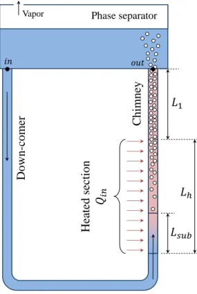
ˆ ascending return branches that conduct the two-phase fluid through a cryostated chimney to a phase separator on top;

ˆ the phase separator, which acts as a liquid reservoir too;

ˆ a down-comer that transports the liquid to feed the modules from the bottom; ˆ a feeder per module.

Figure 1.6(b) shows a diagram of the cooling circuit, where all these elements are explicitly identified. In normal operating conditions, the circuit contains a total liquid helium inventory of 600 l, half of it in the separator and the other half in the heat exchanger region.

1.4.2 The GLAD superconducting spectrometer for R3B

R3B is an international collaboration for the realization of experiments aiming to study reactions with relativistic radioactive beams. The aim of the R3B is the development and construction of a versatile reaction setup with high efficiency, acceptance, and resolution for kinematically complete measurements.

A central role at the R3B experiment is played by the GSI Large Acceptance Dipole (GLAD), a superconducting spectrometer. The superconducting coils, the cold mass of the magnet, the instrumentation of the device as well as the integration of the dipole magnet inside its cryostat is in charge of CEA Saclay, in collaboration with industrial subcontractors. The magnet will be involved in all the experiments, both for the study of the structure of exotic nuclei and for the study of nuclear reaction mechanisms (spallation reactions in particular).

The spectrometer uses a very intense magnetic field to separate efficiently the trajectories of heavy particles from protons. The main objectives of the design are:

ˆ a field integral of 4.8 T.m and 24 MJ stored energy;

ˆ great angular aperture, vertical and horizontal, for light charged particles, charged nuclear fragments and non-deviated neutrons;

ˆ large momentum acceptance to allow for the simultaneous detection of protons and heavy beam residues of the same kinetic energy per nucleon produced at the target point in front of GLAD;

ˆ low fringe field, in order to make possible the use of detectors around the target which are sensitive to the presence of magnetic fields.

The GLAD magnet will be soon installed at GSI, Darmstadt, Germany.

With a length of 3.5 m, width of 7 m and height of 4 m, the total weight of GLAD is 55 tons, 22 of which are taken by the cold mass. The magnetic field is achieved by 6 magnets (two on the left, two on the right, one on top and one at the bottom), as can be appreciated in Fig. 1.7(a). The magnets contain 16 km of NbTi cables, weighing 4.5 tons. The current density is going to be limited to 80 A/mm2, which gives a total current in the coils of 3584 A.

The magnet cooling is provided by conduction of heat through the winding to a two-phase helium flow working in natural circulation configuration [25]. This loop is formed by elements

Mechanical support Vacuum vessel Cooling tubes Collector manifolds

(a) Art work of the cold mass.

Phase separator cryostat

(GHe+LHe)

Cryogenic chimney

CB-2 CB-1 CB0 _CB+1

LHe supply pipe  60.3 x 1.6 Down-comer

5 LHe/GHe return pipes  48.3 x 1.6 Inlet manifolds (feeder) ( 45 x 2.5) Outlet manifolds (collectors) ( 45 x 2.5) CB+2 Heat exchangers (i 14)

(b) Diagram of the circuit.

1.4. Superconducting magnets cooled by natural circulation (a) The GLAD magnets. (b) The GLAD cold mass and co oling system. Figure 1.7. Il lustr ation of the R3B-GLAD systems.