HAL Id: hal-01302829
https://hal.archives-ouvertes.fr/hal-01302829
Submitted on 15 Apr 2016
HAL is a multi-disciplinary open access
archive for the deposit and dissemination of
sci-entific research documents, whether they are
pub-lished or not. The documents may come from
teaching and research institutions in France or
abroad, or from public or private research centers.
L’archive ouverte pluridisciplinaire HAL, est
destinée au dépôt et à la diffusion de documents
scientifiques de niveau recherche, publiés ou non,
émanant des établissements d’enseignement et de
recherche français ou étrangers, des laboratoires
publics ou privés.
Modal and non-modal evolution of perturbations for
parallel round jets
José Ignacio Jimenez-Gonzalez, Pierre Brancher, Carlos Martinez-Bazan
To cite this version:
José Ignacio Jimenez-Gonzalez, Pierre Brancher, Carlos Martinez-Bazan. Modal and non-modal
evo-lution of perturbations for parallel round jets. Physics of Fluids, American Institute of Physics, 2015,
27 (4), pp.044105. �10.1063/1.4916892�. �hal-01302829�
O
pen
A
rchive
T
OULOUSE
A
rchive
O
uverte (
OATAO
)
OATAO is an open access repository that collects the work of Toulouse researchers and
makes it freely available over the web where possible.
This is an author-deposited version published in :
http://oatao.univ-toulouse.fr/
Eprints ID : 15686
To link to this article : DOI:10.1063/1.4916892
URL :
http://dx.doi.org/10.1063/1.4916892
To cite this version : Jimenez-Gonzalez, José Ignacio and Brancher,
Pierre and Martinez-Bazan, Carlos Modal and non-modal evolution of
perturbations for parallel round jets. (2015) Physics of Fluids, vol. 27
(n° 4). pp. 044105-1. ISSN 1070-6631
Any correspondence concerning this service should be sent to the repository
administrator:
[email protected]
Modal and non-modal evolution of perturbations for parallel
round jets
J. I. Jiménez-González,1,a)P. Brancher,2,3and C. Martínez-Bazán1
1Departamento de Ingeniería Mecánica y Minera, Universidad de Jaén, Campus de las Lagunillas, 23071 Jaén, Spain
2INPT, UPS, IMFT (Institut de Mécanique des Fluides de Toulouse), Université de Toulouse, Allée Camille Soula, F-31400 Toulouse, France
3CNRS, IMFT, F-31400 Toulouse, France
The present work investigates the local modal and non-modal stability of round jets for varying aspect ratios ↵ = R/✓, where R is the jet radius and ✓ the shear layer momentum thickness, for Reynolds numbers ranging from 10 to 10 000. The competition between axisymmetric (azimuthal wavenumber m = 0) and helical (m = 1) perturbations depending on the aspect ratio, ↵, is quantified at di↵erent time horizons. Three di↵erent techniques have been used, namely, a classical temporal stability analysis in order to characterize the unstable modes of the jet; an optimal excitation analysis, based on the resolution of the adjoint problem, to quantify the potential for non-modal perturbation dynamics; and finally an optimal perturbation analysis, focused on the very short time transient dynamics, to complement the adjoint-based study. Besides providing with the determination of the critical aspect ratio below which the most unstable perturbations switch from m = 0 to m = 1 depending on the Reynolds number, the study shows that perturbations can undergo a rapid transient growth. It is found that helical perturbations always experience the highest transient growth, although for large values of aspect ratio, this transient domination can be overcome by the eventual emergence of axisymmetric perturbation when more exponentially unstable. Furthermore, the adjoint mode, which excites optimally the most unstable mode of the flow, is found to coincide with the optimal perturbation even for short time horizons, and to drive the transient dynamics for finite times. Therefore, the adjoint-based analysis is found to characterize adequately the transient dynamics of jets, showing that a mechanism equivalent to the Orr one takes place for moderate to small wavelengths. However, in the long wavelength limit, a specific mechanism is found to shift the jet as a whole in a way that resembles the classical lift-up e↵ect active in wall shear flows.
I. INTRODUCTION
The study of round jet stability has been carried out by many authors in the past.1–7In
partic-ular, it has been shown that the selection of the azimuthal symmetry of the most unstable modes depends on the details of the base flow velocity profile. For inviscid flows, it has been analytically determined that fully developed jet profiles,1 characterized by low aspect ratios ↵ = R/✓, where
R is the jet radius and ✓ stands for the shear layer momentum thickness, are only unstable to helical perturbations (azimuthal wavenumber m = 1). On the other hand, when the base flow has a steep velocity gradient,2 in the shape of a “top-hat” profile, the range of unstable azimuthal
wavenumbers is large,8and includes axisymmetric perturbations m = 0, which become the most
unstable for vanishing shear layer thickness.7 It has been found that perturbations with higher
azimuthal wavenumbers m 2 are always more stable than axisymmetric or helical perturbations. Similar instability properties have been shown for fully developed and top-hat jets when considering viscous flows,4although growth rates are smaller for low Reynolds numbers9due to the stabilizing
e↵ect of viscosity.1
The two extreme cases of fully developed and top-hat profiles show that the stability of round jets is characterized by a transition in the azimuthal symmetry of the most unstable azimuthal mode, between m = 1 and m = 0 when the velocity profile sti↵ens. This competition between azimuthal modes has been partially studied in temporal stability analyses,10 though the transition has never
been quantitatively identified. In this context, it should be noted that a spatiotemporal inviscid analysis was performed by Coenen et al.11 for light jets. This study found important di↵erences
in the properties of dominant azimuthal modes of instability when the length of the nozzle from where the jet emerges (a parameter characterizing the jet profile) and the jet-to-ambient density ratio are modified. However, in order to complete our quantitative knowledge of homogeneous round jets instability, a parametric study on the temporal behavior of azimuthal perturbations is therefore needed, with a focus on the influence of the steepness of the jet velocity profile.
The stability of round jets can be analyzed through di↵erent techniques of investigation. The classical temporal stability approach predicts the asymptotic long-time behavior of modal pertur-bations that grow or decay exponentially. But it fails to capture the short-time flow response to disturbances and the potential transient growth of perturbations which might eventually trigger a by-pass transition if the growing disturbances enter the non-linear regime. The possibility of transient growth is correlated with the non-normality of the linearized Navier-Stokes operator, as shown in the case of wall shear flows12 or vortex flows,13 for instance. The study of the transient
dynamics of perturbations therefore involves specific, non-modal analyses14and a global discussion
of the results obtained by the modal and non-modal analyses is necessary to describe consistently the stability properties of a given flow. Di↵erent physical mechanisms are involved in the tran-sient growth phenomenon in shear flows. One is the Orr mechanism,15 which corresponds to the
reorientation of two-dimensional vortical structures initially inclined against the shear that inject energy by rearranging along it. Another transient growth mechanism is the lift-up e↵ect,16,17which
consists in the development of intense streamwise velocity streaks due to the reorganization of the flow by streamwise counter-rotating vortices. A recent work on spatially developing incompressible jets18has found that the largest transient energy gains were due to helical perturbations, leading the
authors to suggest that a type of lift-up mechanism could be involved. A similar conjecture has been made for round viscous jets,19based on the amplification of the streamwise velocity component of
the jet. By contrast, results on the optimal forcing of jets suggest the contribution of an Orr-type mechanism to the perturbations growth.20In that general context, the lack of firm evidence of both
the lift-up and Orr mechanisms in round jets is a strong motivation for a detailed investigation of the non-modal stability of round jets. More precisely, in addition to the clarification on the relevant growth mechanisms, the analysis of the optimal perturbations that benefit from the transient growth could reveal important di↵erences on how axisymmetric or helical disturbances eventually dominate the flow evolution, depending on the characteristics of the jet velocity profile.
The present paper aims at revisiting the local stability of parallel round jets, with an emphasis on the influence of the jet velocity profile on the competition between the axisymmetric (m = 0) and helical (m = 1) perturbations, in a both modal and non-modal framework. This study can be considered as a first attempt to characterize the kind of structures that would be eventually promoted when the profile varies continuously in a downstream evolution of the jet from the nozzle. First, the classical (modal) temporal stability analysis of round jets is complemented by a parametric study that allows to determine the critical value of ↵ above which the structure of the most unstable mode switches from axisymmetry (m = 0) to helical (m = 1) azimuthal symmetry, for di↵erent Reynolds numbers. This part of the study is used as a reference and compared later to results obtained by means of non-modal stability techniques, namely, optimal excitation and optimal perturbation anal-yses. These analyses will allow to quantify how the non-normality of the linearized Navier-Stokes operator can foster transient energy growth, and to identify the perturbations that benefit the most from this phenomenon, depending on the aspect ratio. The competition between axisymmetric and
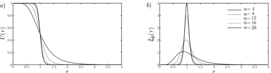
FIG. 1. Base flow velocity (a) and vorticity (b) profiles for di↵erent values of the aspect ratio ↵ = R/✓. R and ✓ are the jet radius and momentum thickness, respectively.
helical disturbances, for a wide range of parameters, will therefore be discussed in the light of both modal and non-modal perturbation dynamics, and the underlying growth mechanisms will be presented.
The paper is organized as follows: the problem formulation and technical aspects are presented in Sec.II. Results are presented in Sec.III, with a quantification of the competition between the unstable azimuthal modes through a modal stability analysis (Sec.III A), followed by results of optimal excitation and optimal perturbation analyses (Secs. III B and III C, respectively) for both m = 0 and m = 1 azimuthal wavenumbers. The transient growth mechanisms are discussed in Sec.III D. The paper ends with the conclusions and perspectives in Sec.IV.
II. PROBLEM FORMULATION AND TECHNICAL BACKGROUND A. Base flow
The base flow consists of an axisymmetric parallel jet whose velocity components and pressure can be expressed in cylindrical coordinates (r, ,z) as U = U(r) ez and P = P(r). In the present
study, the physical quantities are nondimensionalized by the jet radius R and the jet centerline velocity Uj, as the characteristic length and velocity. This choice defines the Reynolds number
Re = UjR/⌫, where ⌫ is the kinematic viscosity of the fluid, as one of the two dimensionless control
parameters of the flow. The other control parameter is the aspect ratio, ↵ = R/✓, defined by the ratio between the jet radius R and the shear layer momentum thickness ✓, where, in dimensional variables
˜r and ˜U, ✓ = ⌅ 1 0 ⇥1 ˜ U(˜r)/Uj⇤ ˜U(˜r)/Ujd ˜r. (1)
The velocity profile is chosen as (Fig.1)
U(r) = 12 ( 1 + tanh " ↵ 4 1 r r !#) . (2)
The dimensionless base flow determined by Eq. (2) corresponds to the family of velocity profiles also used by Michalke.21The shear layer becomes steeper as the aspect ratio ↵ increases,
leading to higher peaks of azimuthal vorticity ⇠ = dU(r)/dr, as shown in Fig.1(b). These ve-locity profiles will be considered as steady base flows, so that the local stability analysis can be performed under the classical assumption of a frozen parallel flow.
B. Linearized problem
The linear stability analysis considers the evolution of infinitesimal perturbations of the base flow, with velocity u0=(u0
r,u0,uz0) and pressure p0. The system invariance with respect to the
(u0,p0) = [u(r,t), p(r,t)] exp[i(m + kz)] + c.c., where u = (u
r,u ,uz) and p correspond,
respec-tively, to the velocity and pressure amplitudes, m (integer) is the azimuthal wavenumber, k (real) is the axial wavenumber, and c.c. denotes the complex conjugate.
Expressing uz and p as functions of u and ur, the linearized incompressible Navier-Stokes
equations can be written in terms of the compact variablev = (ur,u )Tas follows:
F(v) = L@v@t +Cv 1
ReDv = 0, (3)
with L, C, and D linear operator matrices defined in AppendixA, where the partial derivatives @/@ and @/@z have been substituted by im and ik, respectively. The problem formulation is closed with the appropriate boundary conditions for the perturbations, namely, regularity at the origin and decay at infinity.
C. Modal stability analysis
The initial value problem defined by Eq. (3) can be tackled di↵erently depending on the choice for the time horizon of the perturbation evolution. The classical linear stability approach assumes an asymptotic time behavior of the perturbations by considering long-time solutions in the form v(r,t) = ˆv(r) exp( i!t), corresponding to modes of complex frequency !. The real part !r=<(!) is the mode angular frequency and the imaginary part !i ==(!) is the perturbation
growth (!i>0) or decay (!i<0) rate. This exponential time dependence leads to the following
generalized eigenvalue problem:
C 1
ReD !
ˆ
v = i!Lˆv, (4)
where ! is the eigenvalue. The solution of Eq. (4) will provide the asymptotic modal stability properties of the flow at large time horizon.
D. Non-modal stability analyses
A complementary approach is to look for optimal perturbations, i.e., the initial conditions that maximize the gain of energy at a given time horizon t = ⌧, where the gain is defined as the ratio between the perturbation kinetic energy at the final time ⌧ and that at initial time t = 0,
G(⌧) = E(⌧)E(0), (5) with E(t) = 12 ⌅ 1 0 | ˆur(r,t)| 2+| ˆu (r,t)|2+| ˆu z(r,t)|2 r dr. (6)
1. Adjoint system and optimal excitation
In the context of optimal perturbation analysis, it is useful to introduce the adjoint system of the linearized Navier-Stokes operator of Eq. (3). The Lagrange identity22can be used to derive the
adjoint system in the compact form as F+
(a) = L@a@t +C+a 1
ReDa = 0, (7)
wherea = (ar,a )Tare the so-called adjoint perturbations. Here, C+represents the adjoint operator
of C, and L and D are the operators already defined in the direct system (Eq. (3)).
The adjoint initial value problem can be solved as previously, by considering solutions in the forma(r, ,z,t) = ˆa(r) exp [i(m + kz !+t)]. This leads to a generalized eigenvalue problem
similar to that defined in Eq. (4). The relation between the eigenmodes ˆa of the adjoint problem and the eigenmodes ˆv of the direct problem, and their growth rates, can be found by using the
biorthogonality condition.22For a given set of k and m wavenumbers, a direct mode ˆv of complex
frequency ! is associated to the adjoint mode ˆa of complex frequency !+= !⇤, which is the
complex conjugate of !.
It has been shown that the optimal initial condition for large time horizons ⌧ ! 1, for two-dimensional instabilities governed by the Orr-Sommerfeld equation, is the adjoint mode of the most unstable mode of the flow.23 This result has been later generalized for the linearized
Navier-Stokes equations, using a two-dimensional base flow and a three-dimensional perturbation.24
Therefore, this specific initial condition can be interpreted as the optimal excitation of the most unstable mode, which eventually emerges after a transient with an extra gain that can be quantified at large times by ⌘(t) = Go p(t) Gmu(t) ⇡ G+ (t) e2!it 1, (8)
where Gmu(t) and Go p(t) are the energy gains when the initial condition corresponds to the most
unstable mode, or the optimal perturbation at time horizon t, respectively, and G+
(t) is the energy gain given by the time evolution of the initial optimal excitation, i.e., the adjoint mode of the most unstable mode, whose growth rate will be denoted !i hereafter. If the most unstable mode and its
adjoint are, respectively, denoted by ˆvmaxand ˆamax, the energy gain reached after a transient by the
optimal excitation of the most unstable mode can be computed using the general expression derived by Ortiz and Chomaz24for large time,
ln G+ (t) = ln " 1 (ˆv1,aˆ1)2 # +2 !it, (9)
where ˆv1=vˆmax/kˆvmaxk and ˆa1=aˆmax/kˆamaxk corresponds to the normalized modes, and (ˆv1,aˆ1) is
the inner product defined as
(ˆv1,aˆ1) =
⌅ 1 0 vˆ
⇤
1· ˆa1rdr + c.c. (10)
The second term on the right-hand side of Eq. (9) is associated with the energy gain at time t of the most unstable mode, when directly injected at initial time t = 0, and the first term can be related to an extra gain due to transient growth when the initial perturbation consists of the adjoint mode. This leads to the following prediction for the extra gain for large time horizon, t ! 1:
⌘1= 1
(ˆv1,aˆ1)2. (11)
2. Optimal perturbation analysis
If the adjoint-based optimal excitation at large times is a measure of the potential for transient growth, it is also interesting to analyze the optimal perturbation that maximizes the energy gain at shorter time horizons. This optimization problem can be solved using the technique described by Corbett and Bottaro.25The problem involves maximizing the energy gain, defined in Eq. (5), as a
target function, constrained by the linearized Navier-Stokes equations and the associated boundary conditions, using the perturbation at initial time t = 0 as the control variable. Following Corbett and Bottaro,25we introduce the Lagrangian functional
L(v,v0,a,c) = G(⌧) hF(v),ai (H(v,v0),c), (12)
where a(r,t) and c(r) are the adjoint (or co-state) variables that work as Lagrange multipliers. The last term imposes the initial condition, which must match the control condition, H(v,v0) =
v(0) v0=0. In Eq. (12), the term (H(v,v0),c) represents the inner product of H(v,v0) and c as
defined earlier, and
hF(v),ai = ⌅ ⌧ 0 ⌅ 1 0 F(v) ⇤· a r drdt. (13)
The problem reduces to find the set of variables (v,v0,a,c) corresponding to a stationary
Lagrangian functional, L, by setting to zero the directional derivative with respect to an arbitrary variation in the set of variables. In the case of the state variablev, the adjoint system expressed in Eq. (7) arises for the co-state variable,a. Additionally, by setting to zero this derivative with respect tov, both the transfer condition between direct and adjoint systems at t = ⌧,
a(⌧) = E2
0v(⌧), (14)
and the compatibility condition,
c = La(0), (15)
are obtained. Besides, the optimality condition can be derived by combining the result of thev0
derivative of L, c = 2Et E0v0, (16) and Eq. (15), v0=1 2 E2 0 E⌧a(0). (17)
On the other hand, the two remaining variations of L, with respect to a and c, recover the con-straints F(v) = 0 and H(v,v0) = 0, respectively. The strategy followed is an iterative algorithm that,
starting from any initial condition, integrates the direct system first from t = 0 to t = ⌧, followed by an integration of the adjoint system backwards in time, after applying the transfer condition Eq. (14). At that stage, the optimal condition Eq. (17) provides a new guess to iterate again. Convergence is generally achieved within 4 or 6 iterations.26
E. Numerical aspects
The numerical method used in this work is the same as that used by Antkowiak and Brancher13,26
to study the stability properties of a Lamb-Oseen vortex. The reader is referred to these papers and Antkowiak27for the details, validation, and convergence issues. However, some numerical aspects
along with convergence tests are briefly described in AppendixB. In order to accurately solve the direct and adjoint eigenvalue problems, a pseudospectral Chebyshev technique has been imple-mented.28The radial coordinate is discretized as a mapping of the Gauss-Lobatto grid points, by
applying an algebraic function29to adjust the grid into a distribution of points along a semi-infinite
domain. This grid and the di↵erentiation matrices were computed with the DMSuite package writ-ten in MATLAB by Weideman and Reddy.30In order to avoid the geometric singularity at the axis
r = 0 and to force the regularity of the solution in its neighborhood, the parity properties of func-tions with azimuthal dependence of the form exp(im ) have been used, ensuring the smoothness of the solution near the axis.31
III. RESULTS AND DISCUSSION A. Temporal modal stability analysis
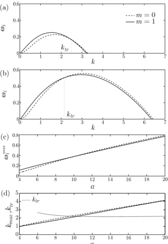
Figures2(a)and2(b)display the growth rate of the most unstable modes of instability for each wavenumber k for m = 0 and m = 1, Re = 1000, and two di↵erent aspect ratios (↵ = 7 and 14, respectively). For ↵ = 7 (Fig.2(a)), the helical mode m = 1 has the largest growth rate, being the most unstable. However, for a larger aspect ratio, ↵ = 14, the most unstable mode is axisymmetric as shown in Fig.2(b). In fact, Fig.2(c) displays the maximum growth rate !max
i for both m = 0
and m = 1, where it can be observed that the unstable modes correspond to shear layer modes, and that both growth rates scale linearly with the aspect ratio in the limit of large ↵.7For a given
FIG. 2. Growth rates of the most unstable azimuthal modes at m = 0 (dashed curve) and m = 1 (solid curve) for aspect ratios ↵ =7 (a) and ↵ = 14 (b) for a jet of Re = 1000. Evolution of the maximum growth rate !max
i with the aspect ratio, for m = 0
and m = 1 (c). Evolution of the wavenumbers of maximum growth rate kmax, and of the transition wavenumber kt r(d).
largest growth rate, !max
i (m). As for the maximum growth rate, kmaxscales as the aspect ratio ↵ for
both azimuthal modes (Fig.2(d)). Also note that the cut-o↵ wavenumber kc(m) corresponding to
the axial wavenumber at which the growth rate decreases to zero also scales as the aspect ratio ↵, see Figs.2(a)and2(b).
The stability curves of Figs.2(a)and2(b)show that the helical perturbations are always more unstable than the axisymmetric ones at low wavenumbers, below a critical wavenumber denoted by kt r on both figures. Reciprocally, the axisymmetric modes are found to be more unstable than the
helical modes above kt r. Figure2(d)presents the evolution of this transition wavenumber kt r(↵) as
a function of the aspect ratio ↵. For low values of ↵, kt r initially decreases with ↵ until it reaches
a constant value of about 2.2 for ↵ > 10 approximately, which is in contrast with the monotonous increase of the most unstable wavenumbers kmaxfor both m = 0 and m = 1.
For very small aspect ratios ↵ < 2, the only unstable mode is the helical one. Above this threshold, the axisymmetric mode becomes unstable as well. More precisely, the bigger the aspect ratio, the more azimuthal modes become unstable (data not shown). This is true in the limit of high Reynolds numbers, and more generally, the number of azimuthal modes that become unstable with increasing aspect ratios depends on the Reynolds number. For instance, at Re = 100 and ↵ = 20, only m = 0, 1, 2, and 3 are found to be unstable while at Re = 1000, unstable azimuthal modes up to m = 7 are observed, indicating the stabilizing e↵ect of viscosity for high azimuthal wavenumbers. This e↵ect is also accompanied by a decrease in the growth rate of the unstable perturbations, although it does not have the same quantitative impact on both m = 0 and 1, which remains the two most unstable modes for all Re.
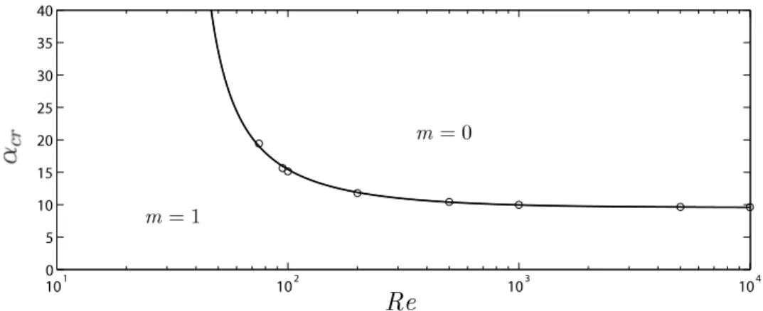
FIG. 3. Critical aspect ratio ↵c r(Re) above (respectively, below) which the most unstable mode is axisymmetric
(respec-tively, helical).
The results shown in Figs.2(a)and2(b), obtained at Re = 1000, suggest that for this Reynolds number, there is a critical aspect ratio ↵crbetween 7 and 14 above which the dominant azimuthal
mode changes from m = 1 to m = 0 (!max
i (m = 0) > !maxi (m = 1)). The critical aspect ratio has
been precisely computed for Reynolds numbers ranging from 10 to 104, and its evolution as a
function of the Reynolds number is shown in Fig.3. The curve ↵cr(Re) defines a border between
two regions in the parameter space within which the dominant mode is either helical (below) or axisymmetric (above). This curve can be approximated by ↵cr(Re) = 390/(Re 33.8) + 9.56, and
presents two limits: ↵cr ! 9.56 as Re ! 1 and ↵cr ! 1 as Re ! 33.8 . Thus, for a
combi-nation of parameters (↵, Re) falling within the region above the curve, the flow will develop vortex rings (for the wide unstable range k > kt r), as a consequence of the jet destabilization through the
most unstable perturbation, which is axisymmetric in that case. On the other hand, if the pair (↵, Re) corresponds to the region dominated by m = 1 modes (i.e., below the curve), the flow is expected to develop mostly a helical structure (except for the narrow unstable range kt r<k < kc).
B. Optimal excitation
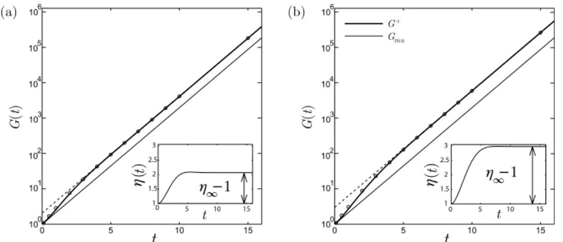
The potential for transient energy growth in perturbed round jets is illustrated in Fig.4, which compares the time evolution of energy gain for di↵erent initial conditions for ↵ = 10 and Re = 1000, and azimuthal symmetry m = 0 (Fig.4(a)) and m = 1 (Fig.4(b)). In both cases, the wavenumber corre-sponds to kmax, at which the respective modes reach their maximum growth rate, namely, kmax=2.30 for m = 0 and kmax=2.13 for m = 1. When the most unstable mode is injected as an initial condition (thin solid line), the time evolution of the energy gain follows exactly the prediction by modal stability analysis, given by Gmu(t) = exp(2!it), with !i>0 being the growth rate of the mode. On the other
hand, when the initial condition is the adjoint of the most unstable mode, the energy gain G+
(t) (thick solid line) undergoes a rapid initial growth before reaching an asymptotic exponential growth parallel to the growth of the direct mode, after t ' 4 for m = 0 and t ' 5 for m = 1 when the perturbation has eventually evolved into the most unstable mode. The growth of the adjoint mode is characterized by an extra gain compared to the growth of the direct mode when the latter is directly injected at initial time. This extra gain ⌘(t) = G+
(t)/Gmu(t) reaches a factor 2 to 3 for m = 0 and m = 1, respectively,
which is an evidence of transient energy growth mechanisms at play in round jets. It is also consistent with the role of the adjoint as the optimal excitation of the most unstable mode. For this specific case, the potential for transient growth is, therefore, more pronounced for helical optimal excitations than for axisymmetric ones. Note that the asymptotic extra gain at large time ⌘1corresponds exactly with
the prediction of Ortiz and Chomaz24given by Eq. (11).
The quantification of ⌘1 for di↵erent axial wavenumbers and Reynolds numbers has been
done through a parametric study, which compares the asymptotic extra gains for di↵erent azimuthal wavenumbers, in order to complement the modal stability analysis and to quantify the influence
FIG. 4. Energy gain for aspect ratio ↵ = 10 and Re = 1000 associated to the most unstable perturbations for (a) m = 0 (k = kmax=2.297) and (b) m = 1 (k = kmax=2.131). The thin solid line (respectively, thick solid line) represents the time evolution of the energy gain of the most unstable direct mode, Gmu(respectively, the energy gain of its adjoint mode, G+),
when injected at initial time t = 0. The dashed line represents the large time asymptotic gain prediction of Eq. (9) for the adjoint mode. The circles correspond to the energy gain of the optimal perturbation computed at the corresponding terminal time. Insets display the temporal evolution of the extra gain ⌘(t) as defined by Eq. (8), and ⌘1corresponds to the asymptotic
prediction of Ortiz and Chomaz24given by Eq. (11).
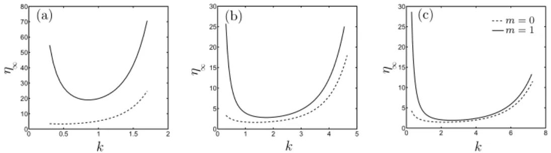
of viscosity, aspect ratio, and axial wavenumber. Figure5displays the extra gain, ⌘1, in the range
of unstable axial wavenumbers k for m = 0 and m = 1 at ↵ = 10 and Re = 100, 1000, and 10 000, respectively. These results confirm that the helical optimal excitations experience a larger transient energy growth than the axisymmetric ones, whatever the axial wavenumber and Reynolds number are. It is noteworthy that transient growth is the most e↵ective for both small and large axial wavenumbers, whereas it is moderate at intermediate wavenumbers. More precisely, the highest gains are obtained for the largest wavenumbers at large Reynolds numbers, for both m = 0 and m = 1 perturbations. These gains are lower when the Reynolds number is decreased due to the stabilizing influence of viscous dissipation for these small length scales. Since the extra gain is associated to the non-normality between the adjoint mode ˆa1and the direct mode ˆv1, this viscous
stabilizing e↵ect at high axial wavenumbers might be associated to a less pronounced spatial sepa-ration between both modes (convective non-normality32) as the Reynolds number decreases (see
Sec.III Dfor details on the nature of such non-normality). For small wavenumbers, or large wave-lengths, the extra gain remains moderate for m = 0 whereas it is large for helical perturbations. Note that in both cases, it does not depend much on the Reynolds number.
The influence of ↵ on ⌘1is displayed in Figure6which plots the extra gain, ⌘1, for a given
Reynolds number (Re = 1000) and three di↵erent aspect ratios (↵ = 4, 10, and 16). As previously observed, the helical perturbations experience the highest transient energy growth for all aspect ratios. The extra gain for axisymmetric perturbations stays at the same levels, and the potential for transient growth shown previously in the axisymmetric case is practically independent on the aspect
FIG. 6. Asymptotic extra gain, ⌘1, in the range of unstable k for Re = 1000 and ↵ = 4 (a), ↵ = 10 (b), and ↵ = 16 (c).
ratio. Only a slight decrease is observed for the largest wavenumbers, correlated with the increasing relative influence of viscous dissipation as the range of unstable wavenumbers increases with the aspect ratio. This e↵ect is also observed for the helical perturbations m = 1. For this azimuthal sym-metry, the influence of the aspect ratio is significant in the whole range of axial wavenumbers. More precisely, transient growth is the most efficient for small aspect ratios, i.e., fully developed jets, with extra gains as large as 20 for moderate axial wavenumbers are observed for ↵ = 4 (Fig.6(a)), while they are ten times smaller for ↵ = 16 (Fig.6(c)).
As mentioned previously, the optimal excitation analysis shows that the potential for transient growth is always larger for helical perturbations, independently of k, Re, and ↵; however, it does not imply that they are the most energetic at all times. Indeed, transient growth induces a larger total energy gain for m = 1 at short times, but if the growth rate of an m = 0 unstable mode is larger than that of m = 1, the axisymmetric mode will eventually emerge as the most unstable, after a critical transition time, denoted hereafter as ⌧t r. This issue is illustrated in Figs.7(a) and
7(b), which present the time evolution of the energy gain for k = 0.3 and k = 4.3, respectively. For k = 0.3, Fig.7(a)shows that the energy gain associated to m = 1 is always larger than the growth corresponding to m = 0. This is consistent with the fact that k = 0.3 is lower than the transition wavenumber kt r' 2.2 in that case (see Sec.III A): the m = 1 unstable mode that emerges has
there-fore a larger growth rate than the axisymmetric one. Since the extra gain is larger for helical optimal excitations, the m = 1 perturbation remains the most energetic for all times. By contrast, the m = 0 unstable mode exhibits the largest growth rate for axial wavenumber k > kt rand, consequently, will
eventually emerge for t > ⌧t r. This can be observed in Fig.7(b), corresponding to k = 4.3, where
it is shown that, during the transient, and shortly in the exponential growth regime until t = ⌧t r,
the helical mode is more energetic than the axisymmetric one. However, after t = ⌧t r, the modal,
long-time, prediction is retrieved with the emergence of the axisymmetric mode.
This result shows that, even if the axisymmetric mode is the most unstable one, the short-time dynamics, dominated by the helical optimal excitation, could lead to a helical bifurcation of the flow if the energy gain for m = 1 was large enough to trigger non-linearities, a phenomenon that would contradict the prediction of the classical temporal stability analysis. In that context, it is interesting to compute the transition time, ⌧t r, in order to quantify the potential for non-linear by-pass transition
FIG. 7. Time evolution of the energy gain of the optimal excitation for ↵ = 10 and Re = 1000 at axial wavenumbers k = 0.3 (a) and k = 4.3 (b). (c) Transition time ⌧t ras a function of k for di↵erent aspect ratios ↵, at Re = 1000.
in terms of timescale: for low values of ⌧t r, the axisymmetric unstable mode emerges too rapidly to
let the transient energy growth at m = 1 activate the helical mode, whereas for large values of ⌧t r,
there could be enough time for the helical mode to be transiently excited and to trigger non-linearities before the axisymmetric mode emerges. As already mentioned, for a given ↵ and k < kt r, the time
evolutions of the energy gains corresponding to m = 0 and m = 1 do not cross, and the transition time ⌧t ris undefined. Consequently, ⌧t rcan be computed only for axial wavenumbers larger than kt r.
Figure7(c)shows the evolution of ⌧t rwith k for Re = 1000 and di↵erent aspect ratios ↵. For all aspect
ratios, ⌧t ris found to decrease monotonously with k, although it slightly increases for the largest k, in
the vicinity of the cut-o↵ wavenumbers kc. As the aspect ratio is increased, the axisymmetric mode
is dominant over a larger range of axial wavenumbers, which corresponds to the widening of the un-stable range of k while kt rbarely changes, and the transition time decreases, leaving less time for the
optimally excited helical mode to by-pass its axisymmetric counterpart. Thus, as a partial conclusion, these results suggest that helical perturbations are more expected to dominate the perturbed jet flow at small wavenumbers (i.e., large wavelengths) and small aspect ratios ↵ (i.e., fully developed jets).
C. Optimal perturbation analysis
An optimal perturbation analysis has been carried out to complement the previous adjoint-based study. The energy gains for di↵erent optimal perturbations are included in Fig.4 as circles located at the corresponding terminal time ⌧ at which the optimal energy gain has been computed. As already mentioned, the transient is relatively short, especially when k is large as shown in Fig. 7(b), since the energy gain reaches rapidly the asymptote given by the optimal excitation prediction provided by Eq. (11). It is observed that the energy gain of the optimal perturbations computed at the terminal times indicated in Fig.4(circles) is quite close to the time evolution of the energy gain G+
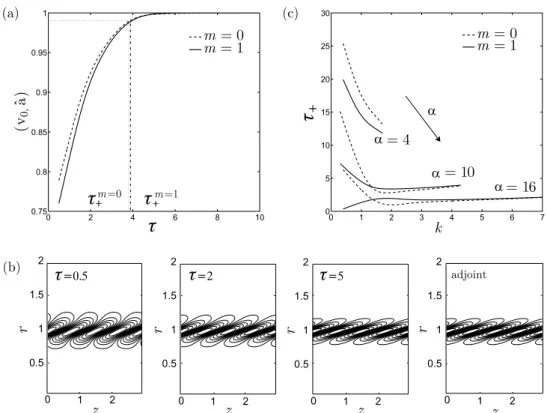
(t) of the adjoint mode (thick solid line). This result indicates that the adjoint mode dominates the transient growth process for the cases studied. A general and objective validation of this hypothesis has been performed through the computation of the inner product between the adjoint mode and the optimal perturbations at di↵erent terminal times. Figure 8(a) presents the evolution of the inner product as a function of the terminal time ⌧ at which the optimal perturbation is computed, for ↵ = 10, Re = 1000, and k = 4.3. As expected, the inner product increases with ⌧ until it eventually becomes unity for large times, which is consistent with the interpretation of the adjoint as the optimal excitation of the most unstable mode, i.e., the optimal perturbation at large time horizon. It is important to note that more than 75% of the structure of the optimal pertur-bation is similar to the adjoint mode for terminal times as low as 0.5. This resemblance between optimal perturbation and adjoint mode is shown in Figure8(b), where the structures (isocontours of azimuthal vorticity) of the optimal perturbations for ⌧ = 0.5, 2, 5, together with that of the adjoint mode (optimal perturbation for ⌧ ! 1) are depicted. As shown in Figure8(a), it is seen that at ⌧ =5, the adjoint of the most unstable mode is already the optimal perturbation.
In order to quantify the domination of the adjoint mode in the short-time dynamics of the per-turbed jet, it is useful to define ⌧+as the time at which the inner product reaches a value of 99%.
Figure8(c)shows the evolution of ⌧+with k for three di↵erent aspect ratios at Re = 1000, where it
can be seen that, for a given aspect ratio, ⌧+decreases when the axial wavenumber k increases, and
that, for large k, the m = 0 and m = 1 perturbations reach the same level of ⌧+. The di↵erence between
the two azimuthal symmetries is more pronounced at small k, when the curvature influence becomes important. In fact, in that range of small k, ⌧+is found to be lower for helical perturbations. It is also
found that the larger the aspect ratio, the smaller the characteristic time ⌧+, which reaches values of
order unity for ↵ = 16. These results suggest that for large aspect ratios, the short-time dynamics of the perturbed jet can be adequately described by the evolution of the adjoint of the most unstable mode.
D. Transient growth mechanisms
The previous results show that transient growth is active in perturbed round jets, especially in the two limits of small and large axial wavenumbers, suggesting that two distinct growth mechanisms
FIG. 8. (a) Inner product between the normalized optimal perturbation and adjoint mode, (v0,a), as a function of the terminalˆ
time at which the optimal perturbation has been computed. ↵ = 10, Re = 1000, and k = 4.3. ⌧+corresponds to the time at
which the inner product reaches 99%. (b) Isocontours of azimuthal vorticity for optimal perturbationsvo, at di↵erent optimal
times ⌧, and adjoint mode ˆa (↵ = 10, Re = 1000, m = 1, and k = 4.3). (c) Evolution of ⌧+with k for ↵ = 4, 10, and 16 at
Re = 1000.
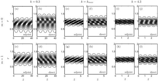
could be involved. Moreover, since the adjoint mode dominates the perturbation dynamics, the phys-ical analysis can be conducted by focusing on the adjoint mode time evolution: at initial time, the perturbation is composed of the adjoint of the most unstable mode into which it eventually evolves after a transient period. These initial and final structures of the perturbation (i.e., the adjoint mode and the associated most unstable direct mode, respectively) are displayed in Fig.9for Re = 1000, ↵ =10, and for both m = 0 and m = 1 at di↵erent axial wavenumbers k.
The dynamics of the perturbation at moderate wavenumber, k = kmax associated to the most
unstable mode, is similar for both m = 0 and m = 1 (Figs.9(e)-9(h)). The initial condition corre-sponding to the adjoint mode consists of azimuthal vorticity structures of alternate signs that are centered at the jet radius (r = 1) and inclined against the shear of the jet (Figs.9(e)and9(g)). The part of these structures that lies within the jet, where the velocities are higher, is advected forward and catches up the part at the outer periphery of the jet. This evolution is similar to that shown by the two-dimensional Orr mechanism in plane shear flows.15In the present case, this mechanism
leads to a transient energy growth for the perturbation, while making it eventually evolve into the most unstable mode (Figs.9(f)and9(h)) associated with the adjoint mode injected as the initial condition. Once locked into the unstable mode, the perturbation behaves in a strictly modal way, i.e., through an exponential amplification, without changing its spatial structure.
The same comments hold for the perturbation dynamics at a higher wavenumber (k = 4.3, Figs.9(i)-9(l)). The main di↵erence lies in the shape of the vorticity structures that are thinner and more inclined. This suggests that the reorientation of these structures due to the shear will be more pronounced, and so will be the transient growth associated with this mechanism. Moreover, the influence of the jet curvature is lowered at a large wavenumber, and therefore the Orr mechanism, which is intrinsically two-dimensional, is expected to be more efficient in that case. These points are
FIG. 9. Isocontours of azimuthal vorticity for the adjoint and direct dominant modes, for m = 0 (top) and m = 1 (down) at axial wavenumbers k = 0.3 (a)-(d), k = kmax(e)-(h), and k = 4.3 (i)-(l), with kmax=2.30 for m = 0 and kmax=2.13 for m = 1.
Here, ↵ = 10 and Re = 1000.
consistent with the large values of extra gain observed for the largest wavenumbers, for both m = 0 and m = 1 (see Figs.5and6).
The scenario is qualitatively di↵erent at large wavelengths, as shown in Figures9(a)-9(d)that correspond to a small axial wavenumber k = 0.3. As previously, the axisymmetric adjoint mode shows azimuthal vorticity structures of alternate signs but that are inclined against the shear only in the outer periphery of the jet (Fig.9(a)). At large wavelengths, the perturbation structure spreads radially within the jet and contaminates the inner potential core that exists for this moderate value of the aspect ratio (↵ = 10). The potential core of the jet corresponds to a uniform velocity flow, where any transient mechanism based on the shear is inhibited. Therefore, the part of the vortical structures that lies within the jet is not a↵ected, and is just advected as a whole, while only the outer part is sheared and reoriented (Fig.9(b)). This dynamics at m = 0, that resembles a truncated Orr mechanism, leads to an energy growth which is smaller than that observed at larger wavenumbers. This is also consistent with the fact that the linearized Navier-Stokes operator becomes self-adjoint in the limit m = 0 and k ! 0.13
For m = 1 (Figs.9(c)and9(d)), the adjoint mode is composed of the same kind of vorticity structures as for higher wavenumbers. These structures are wider radially but do not spread in the potential core as much as their axisymmetric counterpart. Although these structures are completely aligned against the shear, suggesting that their time evolution is similar to the previously analyzed m = 1 perturbations, it should be noted that the associated vorticity distribution corresponds to very elongated vortical structures in the streamwise direction (see the scales in z). Therefore, they di↵er from the nearly azimuthal vortices observed at higher wavenumbers. This is confirmed by the relative levels of azimuthal vorticity of the normalized adjoint modes, which have been measured about ten times smaller at k = 0.3 than at kmax=2.13. The m = 1 perturbation vorticity at low k is found to be
aligned mainly with the streamwise direction, suggesting the importance of analyzing the transient growth mechanism by focusing on cross-sections of the axial vorticity ⇠zin a plane normal to the jet
axis z.
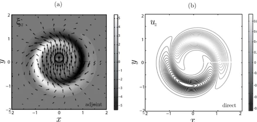
Figure10(a)displays the distribution of axial vorticity associated to the adjoint mode at m = 1 and k = 0.2 for Re = 1000 and ↵ = 10. This initial condition is characterized by the presence of two regions of opposite vorticity facing diametrically and lying in the shear layer of the jet. The velocity field in the cross-section plane associated with this vorticity distribution is displayed as vectors in Figure10(a). As expected from the Biot-Savart theorem, the two counter-rotating streamwise vortex structures induce a velocity field that decays to zero in the far field but that is maximum between the structures. It should be noted that the specific shape of the vortex structures leads to a perturbation
FIG. 10. Cross-section of the adjoint mode axial vorticity ⇠zwith the associated velocity vector field (a). Cross-section of
the direct mode streamwise velocity uz(b). Here, k = 0.2, m = 1, Re = 1000, and ↵ = 10. Light-colored contours stand for
positive values of ⇠zand uz, whereas negative values are represented by dark-colored contours.
induced velocity that corresponds to a virtually uniform flow in the jet. This solid-body translational flow activates a transient growth of energy by shifting up the jet as a whole, as confirmed by the re-sulting mode that eventually emerges after the transient (Fig.10(b)): the axial velocity perturbation associated to this mode shows a velocity increase (respectively, decrease) on the top (respectively, bottom) of the jet, which indeed corresponds to a global upward displacement of the jet. This “shift-up” e↵ect bears some resemblance with the classical lift-up mechanism active in wall flows, where periodic pairs of counter-rotating streamwise vortices lift fluid of low velocity from the wall up in the main stream and reciprocally inject high velocity fluid toward the wall, generating intense streamwise velocity streaks. The present shift-up mechanism acts in a qualitatively similar way, except that only one pair of streamwise vortex structures are involved, and that the entire flow is a↵ected through the radial displacement of the jet as a whole.
It is noteworthy that this shift-up e↵ect is only active in the limit of large wavelengths (or small axial wavenumbers k) since it is based on velocity induction by streamwise, or almost streamwise, counter-rotating vortex structures which are aligned with the axial direction only in the limit k/m ! 0. This is confirmed in particular by Fig.11, which displays the distribution of axial vorticity associated to the adjoint mode for the same parameters’ values as in Fig.10but at a larger wavenumber, k = kmax=2.13. By contrast with the previous initial perturbation at large
wavelengths, the two regions of opposite vorticity are intertwined and overlap each other, leading
FIG. 11. Cross-section of the adjoint mode axial vorticity ⇠zwith the associated velocity vector field for k = kmax' 2.13,
m =1, Re = 1000, and ↵ = 10. Light-colored contours stand for positive values of ⇠z, whereas negative values are represented
to negligible induced velocities in the jet (see vectors in Fig.11). Therefore, the shift-up e↵ect is inhibited, and it is the Orr mechanism which is the relevant one in that case, as described previously (see Figs.9(e)-9(h)). Finally, regarding the e↵ect of the Reynolds number on the transient growth, it can be directly inferred upon evaluation of Fig.5, that viscosity hinders more efficiently the extra gain given by the transient Orr mechanism, acting at high axial wavenumbers, than that provided by the shift-up mechanism at low axial wavenumbers, which is barely a↵ected. Consequently, as the Reynolds number decreases, the spatial separation between adjoint and direct modes becomes less pronounced, resembling the e↵ect of decreasing axial wavenumber depicted in Fig.9.
IV. CONCLUSIONS
A thorough parametric analysis on the local temporal modal and non-modal stability of parallel round jets with varying aspect ratio, ↵ = R/✓, and Reynolds number, Re, has been performed, characterizing the short-time and long-time dynamics of the perturbations. We have focused on the competition between perturbations of azimuthal wavenumbers m = 0 (axisymmetric) and m = 1 (helical), that are known to be the most unstable for top-hat (high ↵) and fully developed (low ↵) profiles, respectively.
A classical temporal modal stability analysis has shown that helical perturbations are always more unstable at a low wavenumber than the axisymmetric ones and, in general, below a critical wavenumber denoted by kt r for all ↵. Reciprocally, the axisymmetric modes have been found to
be more unstable than the helical ones above kt r, for ↵ > 2. When the aspect ratio increases, the
unstable range kt r <k < kc widens, and the axisymmetric mode becomes overall gradually more
unstable. Then, we have determined the critical aspect ratio, ↵cr, for which the general
domi-nant azimuthal perturbation changes from m = 1 to m = 0 (i.e., !max
i (m = 0) > !maxi (m = 1)) for
di↵erent Reynolds numbers. In particular, it has been shown that, in the limit of inviscid flows (Re & 1000), ↵cr' 10, but as Re decreases, the transition takes place at larger aspect ratios, so that
m = 1 becomes the most unstable over a wider range of ↵. However, it should be noted that these viscous results must be interpreted with care due to the limitations of the frozen profile assumption.
The long-time dynamics picture has been completed with studies of adjoint-based optimal excitation and optimal perturbation to evaluate the potential for transient energy growth in round jets. It has been shown that when the initial condition is the adjoint mode, the most unstable mode is optimally excited, and, after a rapid initial growth, the energy gain G+(t) reaches an asymptotic
exponential growth parallel to that of the most unstable global mode, Gmu(t), with an extra gain,24
⌘1, that is always bigger for perturbations with m = 1 for all Re and ↵ investigated, this extra gain being moderate for m = 0.
The higher transient growth anticipated by the optimal excitation study for m = 1 perturba-tions suggested the existence of a transition time ⌧t r determining the critical instant for which
the time evolution of the energy gain of m = 0 perturbations crosses and overcomes that given by m = 1, retrieving therefore the prediction of the asymptotic classical stability analysis (with an extra gain quantified by ⌘1). A parametric optimal excitation analysis has been performed in
order to evaluate the critical transition time for di↵erent values of ↵ and k. It has been shown that transients are in general short, rendering possible to reverse soon the m = 1 dominance given by the short-time dynamics, and observing the unstable m = 0 perturbations emerging at t = ⌧t r, whose
value decreases with increasing ↵. This result is related to a comparative smaller di↵erence in ⌘1
between m = 1 and m = 0, what leaves less time for the optimally excited helical mode to trigger any non-linearities and by-pass the axisymmetric mode. Besides, for all ↵, ⌧t r has been found to
decrease monotonously with k. Therefore, helical perturbations are more expected to dominate the perturbed jet flow at small wavenumbers and small aspect ratios.
On the other hand, the optimal perturbation analysis for Re = 1000 has proven that the adjoint mode drives the transient growth process relatively early, since the asymptotic gain given by Eq. (9) is reached quite soon (see Fig.4). Moreover, a comparison for di↵erent short and finite time hori-zons between optimal initial conditions and the adjoint modes as initial conditions has shed similar values of G(t) (Fig.4), indicating that the optimal conditions and the adjoint modes are similar, and
eventually, at relatively short optimal times, they are nearly identical. In this sense, a quantification of the optimal time for which the adjoint mode starts maximizing G(⌧) has been done with ⌧+,
defined as the optimal time ⌧ for which the inner product between the adjoint mode and the optimal initial condition is 99%. This time is lower than 5 for ↵ & 10, except for small k, so that, for large aspect ratios, the transient dynamics could be properly characterized by the evolution of the adjoint of the most unstable mode.
The previous observation has encouraged us to analyze the transient growth mechanisms focus-ing on the adjoint mode and its time evolution: at initial time, the perturbation consists of the adjoint mode of the most unstable perturbation, which is retrieved after a short transient time. As said before, the short-time dynamics provides with larger energy gains for perturbations with m = 1, for all ↵ and Re investigated. This observation was recently associated18,19to the existence of a mechanism
that resembles the lift-up mechanism. However, the transient growth is especially e↵ective for both small and large axial wavenumbers k, which suggests the existence of two distinct mechanisms. For Re = 1000 and ↵ = 10, we showed that initial conditions corresponding to adjoint modes consisted of azimuthal vorticity structures aligned against the shear, and centered at the jet radius, for moderate and large k. These structures evolve into the most unstable direct modes, as the outcome of an Orr-type mechanism that leads to a transient energy growth, which is more pronounced at large values of k. The latter is related to more inclined adjoint structures, and a lower jet curvature (the Orr mechanism is intrinsically two-dimensional and therefore more e↵ective when the curvature is low). For small wavenumbers and m = 0, the adjoint structures are only partially oriented against the shear in the jet outer part (in the limit k ! 0, the equations are self-adjoint), which renders the mechanism weaker. The scenario is di↵erent for m = 1 and small k. Although the vortical structures resemble those of higher k, they are very elongated in z, and feature lower levels of azimuthal vorticity, the energy being mainly concentrated on the streamwise component of vorticity, ⇠z. An analysis of ⇠z in a
plane normal to the jet revealed two regions of opposite vorticity concentrated in the shear layer, which induce a nearly uniform flow between them in the jet core, shifting the jet upwards as a whole. This “shift-up” e↵ect is similar to the classical lift-up mechanism, and leads to a transient growth of energy by radially displacing the jet, which creates two streamwise velocity streaks of opposite sign whose cores are formed according to the global displacement by the adjoint mode induced cross-section velocity. This mechanism has been shown to be only active for small k, in the limit k/m ! 0, where the vortex structures are aligned with the axial direction, giving rise to large transient energy growth (see Fig.6).
In summary, the present study constitutes an exhaustive analysis of parallel jets instability from a local point of view, that provides with a complete picture of short and long-time stability and retrieves many of the features described in the recent studies. In particular, the combination of local modal and optimal excitation approaches has been proven to be quite accurate to characterize the overall dynamics, including the physical mechanisms behind the transient energy growth, at a low computational cost and without the convergence shortcomings encountered for the global modal approach when the flow is globally stable,18associated to domain truncation and outflow boundary
conditions issues.
ACKNOWLEDGMENTS
This work has been supported by the Spanish MINECO (Subdirección General de Gestión de Ayudas a la Investigación), Junta de Andalucía, and European Funds under Project Nos. DPI2011-28356-C03-03 and P11-TEP-7495, respectively. J.I.J.G. is indebted to Professor Christophe Airiau for his inestimable help and hospitality during his research stays at the IMFT (Toulouse).
APPENDIX A: OPERATORS OF THE LINEARIZED STABILITY PROBLEM
The operators involved in the initial value problem of Eq. (3) are defined as follows:
L = * , 1 0 0 1+-+b1b T 2, (A1)
C = ikU(r) * , 1 0 0 1+-+ikb1U(r)b T 2 b1 @U(r)@r ,0 ! , (A2) D = * , r2m, k 1/r2 2im/r2 2im/r2 r2 m, k 1/r2 + -+b1r 2 m, kbT2, (A3) where bT 1 =ik1 @ @r, im r ! , bT 2 =ik1 @ @r + 1 r, im r ! , r2m, k= 1 r @ @r r @ @r ! m2 r2 k2. (A4)
APPENDIX B: NUMERICAL DETAILS
As reported in Sec.II E, the direct and adjoint eigenvalue problems were solved using a pseu-dospectral Chebyshev technique. More precisely, the infinite radial coordinate was first mapped onto a Chebyshev space, s 2 [ 1,+1], using the Gauss-Lobatto grid, consisting of N points. This grid and the di↵erentiation matrices were computed with the DMSuite30package, and an algebraic
mapping function was applied to adjust the grid into a point distribution so that r 2 ] 1,+1[, taking afterwards only the positive semi-infinite grid, r > 0. This function,
r(s) = s/p1 s2, (B1)
depends upon a stretching factor, , that controls the points spreading after imposing the radius of the penultimate point, rmax, and that is defined through = rmax
q
(1 s22N +1)/s2N +1, being s2N +1
the penultimate point of the Gauss-Lobatto grid. With this transformation, the radial derivatives are calculated as d/dr = d/ds ds/dr, where d/ds is computed with the derivation matrix, and the points 1 and +1 correspond to 1 and +1, respectively. To apply the boundary conditions at s = ±1 (perturbation velocity and its derivative are null), we simply eliminate the first and last columns and lines of the general di↵erentiation matrix dealing only with the internal collocation points, j = 2, . . . ,2N + 1.
It is evident that one of the critical parameter to ensure accuracy of results is the number of points within the shear layer, which a↵ects highly the convergence of the code employed. Because of the mapping, the value will depend on the total number of Chebyshev points, N, and on the maximum radius for the mapping, rmax. To avoid problems of spectral instability and large time
consumption, a moderate value of N is advisable, although it can hinder the accuracy, so that optimal combinations of N and rmaxwere required. In this sense, several issues must be taken into
account. We know that the larger the aspect ratio ↵, the steeper the profiles near the shear layer are, requiring a more compact grid in its vicinity to ensure a smooth solution. As it can be inferred from Eq. (B1), a small rmaxwill ensure a highly clustered grid close to the origin and shear layer.
Nevertheless, if the axial wavenumber, k, is too small, the value of the penultimate point must be increased to map properly the flow, due to the fact that the approximated function decays exponen-tially as r tends to infinity. In this sense, in the limit ↵ ! 1 (cylindrical vortex sheet), the velocity potential eigenfunction1can be expressed as (kr) = DK
n(kr), standing Knfor the modified Bessel
function of the second kind, which decays exponentially as ⇠ 1/pkr e k rwhen r ! 1. Thus, we
might need to increase the number of collocation points to ensure a good resolution in the shear layer, but, as was expressed before, this would go against the computational performance.
Besides, another problem arises when the number of collocation points becomes too large. Spectral methods imply the use of full and ill-conditioned matrices, creating some instabilities when the number of points overcomes some threshold. To work out this contradictory problem of grid parameter choice, we performed some convergence tests for two kinds of base flows: a highly “top-hat” jet (↵ = 30) and a developed profile (↵ = 4). These two values represent the two extreme cases of our parametric study, even though they are far from the critical ratios for which the transitions between the most unstable azimuthal modes take place. Thus, choosing the numerical parameters by analyzing the convergence of these cases ensures the accuracy of the results obtained
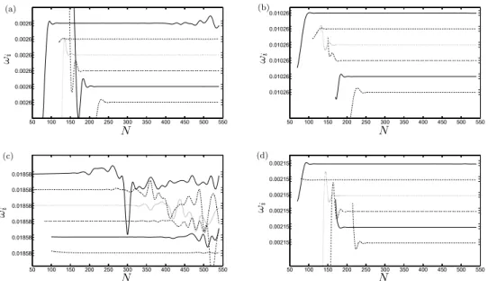
FIG. 12. E↵ect of mapping parameters N and rmaxon amplification factors for ↵ = 30 (Re = 75), (a) k = 0.5 and (b) k = 4.65;
and ↵ = 4 (Re = 10 000), (c) k = 0.1 and (d) k = 2. Each graphic depicts, from top to bottom, tests corresponding to rmax=100,
200, 300, 400, 500, and 800. The ticks around centered values of !idenote an interval !i=±1.5 ⇥ 10 5.
for the rest. On the other hand, to assess the influence of Re, we took advantage of the fact that for smaller Re, the transition takes place for high aspect ratios, whereas for large Re, it occurs for lower aspect ratios, so that we performed the convergence tests at Re = 75 and Re = 10 000 for ↵ = 30 and ↵ =4, respectively.
The tests, aimed at selecting N and rmax, characterized the numerical stability and convergence
of the perturbation growth rate, !i, for the two kinds of base flows mentioned before. The tests
were defined for k = 0.5 and k = 4.65 when ↵ = 30, and k = 0.1 and k = 2 when ↵ = 4, which are axial wavenumbers sufficiently smaller and larger than those of interest in our problem framework, so that the convergence task was representative. We carried out analyses to obtain the evolution of !i as N is increased, for di↵erent rmax, whose results are shown in Fig.12. As it can be inferred
from it, for all rmax, a constant value for !i is reached after some oscillation when N is small, so
that the larger the rmax, the larger the number of points needed for the mode to be converged. It is
proved that there is always an interval in N for which the rmaxcurves overlap, providing the same
results. The upper limit of this interval is imposed by the spectral instability at large N, that gives rise to new oscillations in the value of the amplification rate. This limit appears early for all radii in the case shown in Fig. 12(c), i.e., for the developed jet at Re = 10 000 and k = 0.1, not even converging when rmax=100, indicating how critical this parameter is when the perturbation has a
small axial wavenumber. For the final calculation to be accurate enough, the choice of numerical parameters must lie on the converged limit for all the extreme cases tested, and on the other hand, a small value of N should be selected to reduce the computation time. Taking into account these considerations, N = 200 and rmax=300 stand out as an optimal combination to meet the necessities
and, consequently, were chosen as default values for the present work, providing with accurate results even at high values of Re.
1G. K. Batchelor and E. Gill, “Analysis of the stability of axisymmetric jets,”J. Fluid Mech.14, 529–551 (1962). 2A. Michalke, “On the inviscid instability of the hyperbolic-tangent velocity profile,”J. Fluid Mech.19(4), 543–556 (1964). 3D. G. Crighton and M. Gaster, “Stability of slowly diverging jet flow,”J. Fluid Mech.77(2), 397–413 (1976).
4P. J. Morris, “The spatial viscous instability of axisymmetric jets,”J. Fluid Mech.77, 511–529 (1976).
5A. Michalke and G. Hermann, “On the inviscid instability of a circular jet with external flow,”J. Fluid Mech.114, 343–359
(1982).
6A. Michalke, “Survey on jet instability theory,”Prog. Aerosp. Sci.21, 159–199 (1984).
7M. Abid, M. Brachet, and P. Huerre, “Linear hydrodinamic instability of circular jets with thin shear layers,” Eur. J. Mech.,
B: Fluids12(5), 683–693 (1993).
9M. P. Lessen and P. J. Singh, “The stability of axisymmetric free shear layers,”J. Fluid Mech.60, 433–457 (1973). 10P. Brancher, “Étude numérique des instabilités secondaire de jets,” Ph.D. thesis (Ecole Polytechnique Palaiseau, France,
1996).
11W. Coenen, A. Sevilla, and A. L. Sánchez, “Absolute instability of light jets emerging from circular injector tubes,”Phys.
Fluids20, 074104 (2008).
12P. J. Schmid and D. S. Henningson, Stability and Transition in Shear Flows (Springer-Verlag, 2001).
13A. Antkowiak and P. Brancher, “On vortex rings around vortices: An optimal mechanism,”J. Fluid Mech.578(1), 295–304
(2007).
14P. J. Schmidt, “Nonmodal stability theory,”Annu. Rev. Fluid Mech.39, 129–162 (2007).
15W. M. F. Orr, “The stability or instability of the steady motions of a perfect liquid and of viscous liquid. Part I: A perfect
liquid. Part II: A viscous liquid,” P. Roy. Irish Acad. A27(A), 9–138 (1907).
16T. Ellingsen and E. Palm, “Stability of linear flow,”Phys. Fluids18(4), 487–488 (1975).
17M. T. Landahl, “A note on an algebraic instability of inviscid parallel shear flows,”J. Fluid Mech.98(2), 243–251 (1980). 18X. Garnaud, L. Lessha↵t, P. J. Schmidt, and P. Huerre, “Modal and transient dynamics of jet flows,”Phys. Fluids25, 044103
(2013).
19S. A. Boronin, J. J. Healey, and S. S. Sazhin, “Non-modal stability of round viscous jets,”J. Fluid Mech.716, 96–119 (2013). 20X. Garnaud, L. Lessha↵t, P. J. Schmidt, and P. Huerre, “The preferred mode of incompressible jets: Linear frequency
response analysis,”J. Fluid Mech.716, 189–202 (2013).
21A. Michalke, “Instabilität eines Kompressiblen Runden Freistrahls unter Berücksichtigung des Einflusses der
Strahlgren-zschichtdicke,” Z. Flugwiss.9, 319 (1971).
22D. C. Hill, “Adjoint systems and their role in the receptivity problem for boundary layers,”J. Fluid Mech.292, 183–204
(1995).
23B. F. Farrell, “Optimal excitation of perturbation in viscous shear flow,”Phys. Fluids38(8), 2093–2102 (1988).
24S. Ortiz and J. M. Chomaz, “Transient growth of secondary instabilities in parallel wakes: Anti lift-up mechanism and
hyperbolic instability,”Phys. Fluids23, 114106 (2011).
25P. Corbett and A. Bottaro, “Optimal linear growth in swept boundary layers,”J. Fluid Mech.435, 1–23 (2001). 26A. Antkowiak and P. Brancher, “Transient energy growth for the lamb-oseen vortex,”Phys. Fluids16(1), L1–L4 (2004). 27A. Antkowiak, “Dynamique aux temps courts d’un tourbillon isolé,” Ph.D. thesis (Université Paul Sabatier de Toulouse,
France, 2005).
28B. Fornberg, A Practical Guide to Pseudospectral Methods (Cambridge University Press, 1995).
29C. Canuto, M. Y. Hussaini, A. Quarteroni, and T. Zhang, Spectral Methods in Fluid Dynamics (Springer, 1988). 30J. A. C. Weideman and S. C. Reddy, “A MATLAB di↵erentiation matrix suite,”ACM Trans. Math. Software26(4), 465–519
(2000).
31R. R. Kerswell and A. Davey, “On the linear instabillity of elliptic pipe flow,”J. Fluid Mech.316, 307–324 (1996). 32J.-M. Chomaz, “Global instabilities in spatially developing flows: Non-normality and nonlinearity,”Annu. Rev. Fluid Mech.