Deep Learning to Characterize Ice Stream Flow
by
Brindha Kanniah
Submitted to the Department of Earth, Atmospheric and Planetary Sciences
in Partial Fulfillment of the Requirements for the Degree of
Master of Science in Earth and Planetary Sciences
at the
MASSACHUSETTS INSTITUTE OF TECHNOLOGY
June 2019
@
Massachusetts Institute of Technology 2019. All rights reserved.
Signature redacted
Signature of A uthor ... ..Department of Earth, Atmospheric and Planetary Sciences May 9, 2019
Signature redacted
C ertified by ...Brent Minchew Assistant Professor of Earth, Atmospheric and Planetary Sciences
Signature redacted
Accepted by MASSCHI E NSTUTE OF TICNLGL
JUN
17
2019
LIBRARIES
Thesis SupervisorRobert D. van der Hilst Schlumberger Professor of Earth and Planetary Sciences Department Head
Abstract
The physical properties of glacial beds have tremendous influence over ice flow motion, especially in regions where the ice sheet is shallow and tidally-modulated. In these regions, basal shear stress dominates the force balance of ice sheets, while basal slip along the ice-bed interface is the primary component of ice flow. How-ever, the physical parameters of glacial beds are poorly understood due to limited observational information available, as these beds lie under ice sheets with depths up to a few 1000s of meters. Thus, our research goal is to better understand the mechanics of glacier beds, which will improve out understanding of how ice sheets respond to changing climates and shape the solid Earth.
Specifically, we test if deep learning is a method that is capable of capturing the temporal evolution of ice flow. Our results show that recurrent neural networks built from Long Short-Term Memory units are a promising method for learning os-cillatory patterns in ice stream dynamics. In addition, these networks can function as forecast models which create a sequence of predictions conditioned on past ob-servations. This confirmation paves the way for further research into creating a continuous spatial-temporal model of ice flow, by applying deep learning methods on sparse observational data of glaciers.
Contents
1 Introduction 11
1.1 M otivation . . . . 12
1.2 Extended Research Goal . . . . 14
1.3 Rem ote Sensing . . . . 15
1.4 Geographic Review of the Rutford Ice Stream . . . . 17
2 Review of Ice Sheet Dynamics 19 2.1 M ass Balance . . . . 19
2.2 C reep . . . . 19
2.3 Basal M otion . . . . 21
2.4 The Shallow Stream Approximation . . . . 24
3 Deep Learning 29 3.1 Review of Deep Learning . . . . 29
3.2 Recurrent Neural Network . . . . 31
3.2.1 Recurrence with Perceptron Units . . . . 32
3.2.2 Recurrence with Long Short-Term Memory Blocks . . . . 35
4 Application to Glaciology Research 41 4.1 Structuring Ice Stream Flow for Deep Learning . . . . 42
4.2 Forecast Network . . . . 45
4.2.1 Single-Value Forecast . . . . 4.2.2 M ultiple-Value Forecast . . . .
5 Implementation
5.1 Software ...
5.2 General Workflow . . . .
5.3 Model Workflow and Results . . . .
5.3.1 Single-Value Forecast Model . . . 5.3.1.1 Architecture . . . .
5.3.1.2 Training and Testing . .
5.3.1.3 Validation . . . .
5.3.2 Multiple-Value Forecast Workflow
5.3.2.1 Architecture . . . .
5.3.2.2 Training and Testing 5.3.2.3 Validation . . . .
5.3.3 Discussion of Results...
6 Conclusions and Perspectives
46 49 52 . . . . 52 . . . . 52 . . . . 55 . . . . 56 . . . . 5 6 . . . . 5 7 . . . . 5 8 . . . . 6 2 . . . . 62 . . . . 64 . . . . 66 . . . . 6 7 70
List of Figures
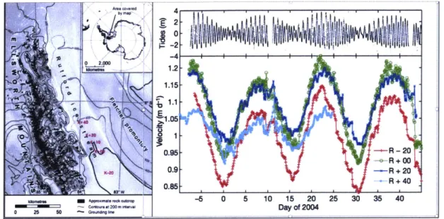
I Left panel shows the location of the five GPS stations in RIS, and the location of RIS in Antarctica (top right). The numbers in the labels K-20 to K+40 refer to the distance of the site from the grounding line (outlined in dark black) The top right panel shows up-direction (vertical) displacements 20km downstream from the grounding lines. The bottom right panel shows surface speed at distances between -20km to 40km the
grounding line. Images from [Gudmundsson, 2007]. . . . . 13
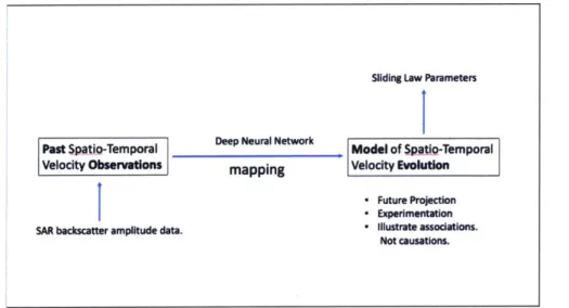
2 Macro-view of extended research goal. We aim to use deep learning as a map between sparse velocity observations to a continuous model of ve-locity evolution, with the final goal of further constraining the siding-law param eters. . . . . 15 3 Horizontal velocity map of the Antarctic ice sheet, generated using SAR
and interferometric-SAR data acquired with a collection of satellites: ALOS
PALSAR, Envisat ASAR, RADARSAT-2, and ERS-1/2. Image from
Rig-not et al. 12011]. . . . . 16
4 Cross-sectional diagrams showing the range of ice sheet heights for West and East Antarctica. Figure from Schoof and Hewitt 120131. . . . . 18 5 Close-up views of RIS. Map in left panel is from Gudmundsson and Jenkins
[2009]. Image on left panel is an optical image of RIS (outlined in red)
created using Google Earth; where we see how RIS is bordered by the Ellsworth Mountains (appearing as grainy texture on the ice sheet) on
one side. . . . . 18
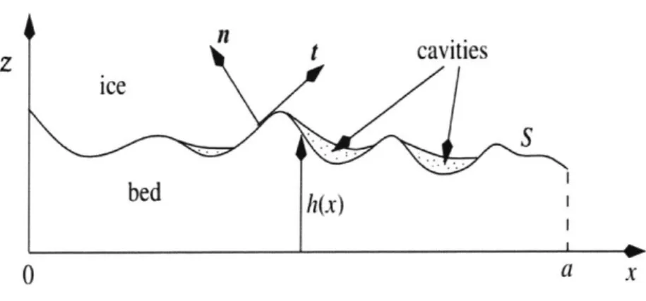
6 Cross-section of glacial bed. Note the notation used to label the coordi-nate directions, the normal and tangential to the bed. This notation cor-responds to the derivation of Tb below. Illustration adapted from [Schoof
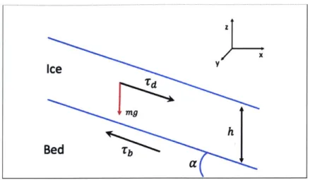
7 Illustration of ice stream, with vertical thickness h, lying on a bed inclined at an angle a to the x-direction. The ice stream has width that spans the y-direction, and height in the z-direction. rd is the downstream driving
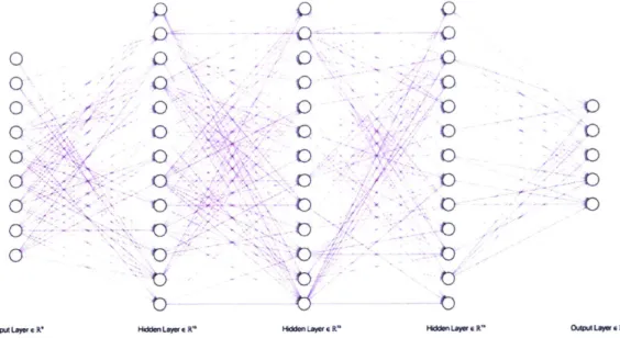
force due to gravity, and Tb is the upstream basal shear stress. . . . . 27 8 Basic Multilayer Perceptron (MLP) network, with an input layer of nine
input nodes, three hidden layers of 13 nodes each, and and output layer of five output nodes. The arrows between nodes represent the weights connecting inter-layer nodes from the previous layer to the subsequent layer. The opacity of each arrow represents the magnitude (strength) of each w eight. . . . . 29 9 Simple RNN network. The image on the left of the equal sign is the
concise representation of an RNN, and the image on the right of the equal sign is unrolled equivalent. In this example, the input a provided are one time step behind the outputs b generated. Thus, this network is designed to make predictions one time-step in the future. . . . . 32 10 Long Short-Term Memory (LSTM) block. Diagram from [Hochreiter and
Schm idhuber, 1997]. . . . . 39
11 Functions used for information flow and control through LSTM block. The function g squeezes input sources directly entering the block, the function
h squeezes the updated cell state, and the function
f
generates control with gated-activation values. Mathematically, these functions are different transformations of the logistic sigmoid: g = 2, h _ -1 and1+ex...40
12 Visualization of input data as discrete points with values vj, in a cube with dimensions in the x, y (spatial) and t (temporal) axes. . . . . 43
13 New dataset is a sliced portion of the original cube in Figure 12. This cuboidal slice has unit area in space at position, (XO, yO), and length ex-tending the entire duration of observation time, t. . . . . 43
14 Sample of synthetic dataset. Each panel shows a time series (representing the displacement equivalent of the cuboidal slices of Figure 13) with daily
GPS measurements over a 14 year time period. The deformation measured
is the instantaneous displacement magnitude (labeled as amplitude in the figure) of a point on the surface of the ice stream. Refering to equation
(1), this deformation quantity could be expressed as Iu(r, t) 1, where r is
the position relative to the GPS station; and t, the instantaneous time of observation. . . . . 44
15 General structure of single-value forecast model. . . . . 46
16 General structure of encoder-decoder model . . . . 49
17 Single-value forecast model predictions for test data time series (with seven year period). While testing and training we implemented a two-layer LSTM block, with two-layers of three different sizes: 120, 80 and 60
LSTM cells (labeled Big Model, Medium Model and Small Model). The
accuracy of the Big Model and Medium Model predictions are quite con-sistent over the entire time period, however the accuracy of the medium model predictions declines slightly towards the end of the time period; predictions slightly overshoot target values. . . . . 59 18 MSE calculated during each training epoch for the three models listed in
Figure 17. The bigger the model, the faster the convergence of the MSE. For all models, the MSE starts to converge around the fourth epoch, reaching a minimum at the fifth epoch. . . . . 60 19 Single-value forecast model predictions for validation data time series.
The predictions follow target values closely. However, there is a slight undershoot (a downwards-shift with respect to the y-axis) of predictions compared to targets. Note the RMSE value of predictions with respect to targets is 0.381. Model residuals are centered at zero, and do not follow a particular pattern. . . . . 61
20 MSE of encoder-decoder model computed during each training epoch. The MSE is approximately 6.5 at the fourth epoch and 5.5 at the tenth epoch,
indicating an average MSE rate of change of about 0.167 per epoch, past the fourth epoch. This rate of change is less drastic than that of earlier epochs before the fourth epoch. . . . . 65
21 Encoder-decoder model predictions for four validation time series. Note the RMSE value of predictions compared to targets, has a minimum of
1.884 (second panel from top) and a maximum of 3.785 (top-most panel).
List of Code
1 Single-value model architecture implementation. . . . . 56
2 Division of data into training and testing sequences. . . . . 57
3 Training of model over 20 epochs. . . . . 57
4 Using trained model to make predictions with test data. . . . . 58
5 Encoder network architecture implementation. . . . . 62
6 Integration of encoder and decoder networks in single model . . . . 63
7 Generating training and testing datasets. . . . . 64
8 Training of encoder-decoder model over 10 epochs . . . . 64
9 Using trained model to make predictions with test data. . . . . 64
1
Introduction
In light of climatic changes and oceanic warming, a prominent question asked is how does ice respond to these changes? This question is important because global sea level rise is largely dependent on the melting of ice sheets' - the two largest ice sheets being those of Greenland and Antarctica. The contribution of the ongoing melt and retreat of Antarctica's ice sheet has been predicted to soon overtake other sources, with a drastic surge in ice discharge that could possibly happen within the next few decades [Scambos et al., 2017; Pollard et al., 2015]. Ice loss from the Antarctic Ice Sheet (AIS) has been projected to have increased by 75 % in the last decade. Most of this loss is localized to the Western Antarctic Ice Sheet (WAIS), and caused by temporal changes in the velocities of ice stream flow (Gudmundsson 2009, Rignot and others 2008); these elements - WAIS and ice stream dynamics - form the overarching region and scope of our investigation.
Discussions of the Polar Research Board (within the National Academies Sciences, En-gineering, and Medicine) in 2015, led to the decision that highest-priority Antarctic research is the study of cause, extent and rate of changes in WAIS - and their impli-cation to sea level rise. This decision was presented in a report NAP21741, which was debated in the National Academies 2016 meeting in Boulder. The 2016 meeting resulted with the outlining of four fundamental questions that define future research in WAIS [Scambos et al., 2017]:
1. Drivers: What factors cause the observed change in WAIS?
2. Boundary Conditions: How can the boundary conditions in WAIS be mapped for predictive modeling and better understanding of its dynamic processes?
3. Processes: What mechanisms are involved in marine ice sheet retreat and collapse?
4. Models: How the resolution and accuracy of future behavior projections in WAIS be improved?
'In addition to glacial melting, sea level rise is caused by the thermal expansion of water due to greenhouse-gas induced global temperature change. See Wigley and Raper [1987], for more information.
Our investigation seeks to answer the questions of Boundary Conditions and Models. First, we examine the boundary condition provided by basal traction and its influence on ice stream flow. Then, we study deep learning as a method to characterize ice stream flow; this study is a step towards the larger goal of elucidating the parameters governing basal traction.
1.1
Motivation
Our study is motivated by the previous work of Minchew et al. [20171, where a Bayesian method was developed for inferring a time-dependent glacial surface velocity field using synthetic aperture radar (SAR) data. The method relied on having prior information about the the form of the basis functions for ice stream displacement,
k[ai
sin wit +
0i1
u(r, t) = 't + 0 sin wit
+
(1)i=1
U sin wit +
#u
where 8, h, f represent the east, north and up, mutually orthogonal coordinate direc-tions; these form the unit directions of all vectors in equation (1). u(r, t) represents the instantaneous displacement vector, located at a position r relative to the observer.
u(r, t) is dependent on v'(r), a long-term non-periodic velocity term; and a family of
sinusoidal functions, with frequency w, amplitude a(r) and phase 0(r).
The form of the displacement equations (1) is applicable to regions where ocean tides have an influence on ice stream flow. Their study focused on the Rutford Ice Stream (RIS) region (described in more detail in Section 1.4), where Global Positioning System
(GPS) displacement observations were collected from five sites in December 2003 to
February 2004 (Figure 1).
These observations confirm that RIS's ice flow velocity is influenced by ocean tides. Fur-thermore, the tides have been shown to cause changes in the horizontal surface velocity up to tens of kilometers upstream from the grounding line (the furthest upstream GPS
-4 1.2
4:
1.15 1.05 \? .95 - -R - 20 --R +00 K-W0.9 - -- R + 20 0.85 - -R + 40 -6 0 5 10 15 20 25 30 35 40 Day of 2004Figure 1: Left panel shows the location of the five GPS stations in RIS, and the location of RIS in Antarctica (top right). The numbers in the labels K-20 to K+40 refer to the distance of the site from the grounding line (outlined in dark black) The top right panel shows up-direction (vertical) displacements 20km downstream from the grounding lines. The bottom right panel shows surface speed at distances between -20km to 40km the grounding line. Images from [Gudmundsson, 20071.
station being 40km from the grounding line) and the largest tidal modulations happen over long tidal periods of 14.76 days due to the fortnightly tidal constituent (MSf) [Gud-mundsson, 20071. Therefore, the displacement equations (1) are representative of the
velocity field of RIS.
The limitation of the Bayesian method of inferring velocity fields however, lies in the need to know the priori form of the displacement equations (1). In the case of RIS, we are confident in the form of the equations because they can be cross-checked against GPS data. However, in glacial regions where ice flow has not been tracked by observation systems and where there is a large uncertainty in its dynamical nature, it is difficult to be certain of the form which the displacement equations take.
Thus, our study seeks to develop a more generalizable method of characterizing glacial ice flow, that does not depend on prior knowledge of the form of the displacement equations. The method of deep learning has shown promising results in learning representations from data belonging to complex systems, specifically those built on compositional hierarchies (a property of many natural signals) [Lecun et al., 2015]. We want to investigate if
this method can be applied to the ice stream system, by testing its ability to learn the evolutionary patterns of ice flow.
1.2
Extended Research Goal
The specific goal of our research is to discover if deep learning is a method that is capable of learning evolutionary patterns of ice flow on the surface of a glacial ice stream. Our reason for choosing ice streams, is because extensive observation and studies have been made on RIS; therefore, we hope that our results may contribute towards further research in modeling and understanding the flow dynamics of RIS.
Our specific research goal belongs to the larger research area of understanding the me-chanics of the ice-bed interface. The dynamical property at the interface we are interested in is the basal boundary condition. This boundary condition is typically expressed as the sliding-law (Section 2.3), which takes the form of:
Tb = Cb(2)
where Tb refers to the basal shear stress, and Vb, ice velocity at the bed of the glacier.
The problem of constraining the parameters, C (a constant) and the exponent , has
been a long-withstanding problem in glaciology [Minchew, 2018b]. A solution however might be in assuming the constancy of C and - over a specific spatio-temporal spacen and taking repeated measurements of Vb over this space, to perform a regression
anal-ysis on the sliding-law. Specifically, by substituting Vb measurements into the Shallow Stream Approximation equations (SSTREAM); a set of coupled differential equations describing tidally-modulated ice stream flow (see Section 2.4 for a detailed description); the SSTREAM equations are reduced to one unknown, Tb. Hence, rb can be solved for
at every instance in time at which Vb is measured. Finally, by inferring r and observing
Vb, a linear regression can be performed on the logarithm of equation 2 to constrain the
values of C and '.
log10 o b log10 (3)
1
logio b = log10 o C + -nlogo Vb
However, velocity measurements of glacial regions are often sparsely taken in time, and therefore we are interested in creating a continuous model of the spatio-temporal evolu-tion of Vb, based on sparse surface velocity measurements, for a more accurate regression analysis on the sliding-law (Figure 2). This is our extended research goal, which serves to streamline the scope of our study.
Sliding Law Parameters
Past $pWW-Temporal Deep Neural Network Model of SpWtig-Temporal
velocity Observations mapping VelocIty EvolutIon
9 Future Projection
- Experimentation SAR backscatter amplitude data. * Illustrate assodations.
Not causations.
Figure 2: Macro-view of extended research goal. We aim to use deep learning as a map between sparse velocity observations to a continuous model of velocity evolution, with the final goal of further constraining the siding-law parameters.
1.3
Remote Sensing
Basal shear stress has a direct influence on the velocity field of glaciers. This relationship is derived in Section 2.4, where the forces due to basal traction at the glacial sole and forces due to gravity over the depth of the ice, act to create spatial gradients in the horizontal surface velocity field.2
Therefore, to understand and parameterize basal shear stress, the spatial gradients in the horizontal velocity field must be resolved. One method of doing so is to generate a region-wide map of the velocity field (containing horizontal velocity vectors on a grid of discrete points in space), and then applying a simple differential algorithm that would calculate the spatial gradients of velocity at the grid points.3 An example of a region-wide
2
The relationship between velocity gradients, driving force and basal force is expressed in the SSTREAM approximation (equations 30 and 31, Section 2.4).
velocity field map is shown in Figure 3, that of the Antarctic continent.
A well-developed way to generate surface, horizontal velocity field maps is by using
synthetic aperture radar data acquired from airborne or spaceborne antennas surveying the region of interest. The acquisition of SAR data is this form is called active remote sensing, whereby an antenna actively sends out electromagnetic waves (usually falling in the microwave frequency range) to a terrain and receives the backscatter waves. The energy contained in the backscatter is dependant on properties of the scatterer surface subsurface volume, in addition to the emitted-wave polarization and imaging geometry of the airborne antenna [Minchew, 2018a].
v'ocity magnitude [mr 0
1000W
<1.5 10 100 1000
-.1280
Figure 3: Horizontal velocity map of the Antarctic ice sheet, generated using SAR and interferometric-SAR data acquired with a collection of satellites: ALOS PALSAR, Envisat ASAR, RADARSAT-2, and ERS-1/2. Image from Rignot et al. [2011].
From the SAR datasets available at Vertex, the Alaskan Satellite Facility's database, an ongoing radar survey of the ice streams flowing into the Ronne Ice Shelf (one of which is
the region since 2016), developed by the European Space Agency (ESA). In addition to providing data products, the ESA also provides a software toolbox for analyzing the data: The Sentinel 1 Toolbox (SITBX) can be downloaded from the ESA Sentinel website, and contains a collection of processing tools, data product readers and writers, and a display and analysis application. By taking pairs of high-resolution Interferometric Wide Swath (IW) Sentinel-i Level-1 Ground Range Detected (GRD) data over the RIS region, a cross-correlation algorithm can be applied on them using the Offset Tracking program in SITBX. This algorithm would compare the image pair and match selected Ground Control Points (GCPs) within the images.4 The offset between the GCP pairs is the horizontal displacement of that point within the time period of image acquisition. The displacement vectors, which are two dimensional in the x-y horizontal plane, would then be scaled (by division) with the acquisition time interval to calculate the horizontal velocity vectors of the GCP grid. The GPC grid would subsequently be interpolated to compute the velocity vectors of the region-wide pixel grid; to thereby generate a velocity field map of the RIS region.
1.4
Geographic Review of the Rutford Ice Stream
The Antartic ice sheet is a continent-scale mass of glacial ice, with surface elevations that range from 0km to about 4km above sea level (Figure 4). In West Antarctica, the ice sheet rests on a bed well below sea level and often terminates in ice shelves that float on the ocean. Within the Antartic ice sheet are ice streams, defined as regions that flow more rapidly than the surrounding ice [Bentley, 1987]. Bentley provides two insights from this definition: First, ice streams are bordered by ice (not by rock). Second, ice streams are in contact with bedrock (not floating on seawater), because they are part of an inland ice sheet.
The Rutford Ice Stream (RIS) lies on the West Antartic Ice Sheet (WAIS), and is bor-dered on one side by the Ellsworth mountains and on the other by smooth-surface low-lying ice. RIS belongs to a family of ice streams, the Ronne ice streams, which flow into the Ronne Ice Shelf. See the left panel of Figure 1 for locating RIS's position in
I SU
2 0
-(MSL0 Ronne Ice Shelf--1
West AntArctic.a
Ross Ice Shef B' k M LOWd 111111 On BM t lallT.sh 21000
Aurora Vincinruss Astrolabe Sssislacila Basin SssbgladalI Basin SubgLacial Bassn
Figure 4: Cross-sectional diagrams showing the range of East Antarctica. Figure from Schoof and Hewitt [2013].
ice sheet heights for West and
Antarctica, and see Figure 5 below for a close-up view of RIS.
500 Rw
ON
(/6
Mauf-We~di sea
M-Figure 5: Close-up views of RIS. Map in left panel is from Gudmundsson and Jenkins
[20091. Image on left panel is an optical image of RIS (outlined in red) created using
Google Earth; where we see how RIS is bordered by the Ellsworth Mountains (appearing as grainy texture on the ice sheet) on one side.
I
00
0
-0
2
Review of Ice Sheet Dynamics
The varied mathematical models that describe ice sheet dynamics are built from funda-mental concepts. Here we present a few of these fundafunda-mental concepts that help give us a general understanding of the sustainence and large-scale flow of ice sheets. In ad-dition, as our study is focused on ice streams, we take a close look at an approximation frequently used in the modeling of ice streams.
2.1
Mass Balance
The mass balance of an ice sheet is the change in total mass of a region of ice over a certain period of time. Over an annual cycle, an ice sheet experiences a winter season and a summer season. A net accumulation of ice due to snowfall happens during winter, and a net ablation of of ice due to melting at the glacial terminus happens during summer [Cuffey and Paterson, 2010; Schoof and Hewitt, 2013]. To sustain the existence of an ice sheet, the mass balance of the sheet has to be a net zero (maintenance) or positive (growth); processes that accumulate ice (primarily, snowfall) must outweigh processes that ablate ice (melt at the ocean-ice interface). These processes are thought of collectively as mass exchanges, which happen at the source and sink respectively. The mass balance of a specific zone within the ice sheet is also influenced by the distribution of mass within the zone, which is caused by the flow of ice from sources to sinks.
2.2
Creep
Glacial ice is a polycrystalline material, composed of 106 to 109 crystal grains (formed from H20 molecules) in a cubic meter of fully-formed ice. The properties of
individ-ual crystals and the interaction between crystals give ice its bulk nature [Cuffey and Paterson, 2010]. The bulk nature of ice over long temporal and spatial scales, is that it deforms as a shear-thinning viscous fluid, meaning that its viscosity decreases under increasing strain rates.
Stemming from this material property of ice, is an important constitutive equation in glacial dynamics, often known as Glen's flow law, a creep relation showing the relation-ship between strain rate and stress. Glen's flow law can be expressed as
eij = An-1riTj, (4)
where r is the effective deviatoric stress 5; Tij, a component of the deviatoric stress tensor;
and Eij, a component of the strain rate tensor. A is called the rate factor, and depends on the properties of ice including temperature, crystal size and impurity content. The exponent n typically ranges from 1.5 to 4.2, but n = 3 is the best fit to empirical data [Cuffey and Paterson, 20101.
Substituting the relationship between strain rate and stress for a Newtonian viscous fluid, with viscosity y (equation 5 below),
E = 1j ij (5)
277
into equation (4), the stress-dependant viscosity of ice can be expressed as,
1
S= 2 1 (6)
By inverting Glen's flow law to express rij = f(A, n, eij, e) and substituting equation (5)
into it, ice's viscosity can be expressed in terms of the effective strain rate e too,6
1 =
A -n . (7)
2
This relationship (7) will be useful in Section 2.4, where we derive the equations of motion for shallow ice streams.
5
The effective deviatoric stress is equivalent to the square root of the second invariant of the deviatoric
stress tensor, T = V-Tr7-/2
6
The effective strain rate is equivalent to the square root of the second invariant of the strain rate
2.3
Basal Motion
Basal shear stress, Tb, is among the main controls to the motion of fast-flowing glaciers. Glacial flow is induced by three mechanisms: polycrystalline creep of ice (Section 2.2), the sliding of ice over its bed and the deformation of the bed itself. The combined motion of the sliding of ice and of bed deformation is called "basal motion" (equivalently "slip", "glacier sole motion") [Cuffey and Paterson, 2010]. With this nomenclature, the three mechanisms of glacial flow can be categorized into two mechanisms: the polycrystalline creep of ice and basal motion.
The motion of the world's fastest glaciers are dominated by basal motion and are mini-mally influenced by the deformation of ice [Morlighem et al., 2013]. To investigate these regions of fast-flowing glaciers, large efforts have been made toward understanding basal motion. However, because the bed of glaciers cannot be directly observed (as they are of-ten submerged under thick sheets of ice), the parameters that characterize basal motion are poorly constrained.
Depending on the nature of the bed, these parameters take on different forms. The two main classes of beds are hard beds and soft beds. A hard bed consists of rigid and impermeable bedrock, whereas a soft bed consists of deformable and permeable bedrock. The classical theory of basal motion considers sliding over a hard bed; of which the first quantitative expression was given by Weertman [1957] [Fowler, 2010]. Weertman proposed the sliding-law, a power-law relationship between the the basal shear stress, Tb,
and basal velocity, Vb, as:
Vb = CTb(8)
An inversion of Weertman's equation (8) leads to
Tb b/ (9)
where c and C are constants of different values. This form of the equation (9) is physically more meaningful because the generator of the basal shear stress, which opposes motion,
is basal velocity [Cuffey and Paterson, 2010].
According to Weertman, there are the two mechanisms by which ice moves along the bed, past obstacles: regelation and enhanced creep.7 Additionally, the Weertman sliding law is based on the following presumptions:
1. Ice rests on a hard bed
2. Ice is near its melting point and a thin film of water forms between the bed below and ice above.
3. There are no cavities on the bed.
4. The surface of the bed has undulations (bumps) that resist ice flow, creating basal drag.
To understand Tb in terms of the stresses, a, at the glacier sole, we refer to Schoof's derivation [Schoof and Hewitt, 2013], outlined below.
z
n
t
cavities
ice
bedh(x)
0
a
x
Figure 6: Cross-section of glacial bed. Note the notation used to label the coordinate directions, the normal and tangential to the bed. This notation corresponds to the derivation of Tb below. Illustration adapted from [Schoof and Hewitt, 2013]
In this derivation, vectors are indicated in bold font, and scalar magnitudes with regular font. We consider the two-dimensional case, where the x and z coordinate axes are
7
For more information on these mechanisms, see [Cuffey and Paterson, 20101.
maintained and the y-axis ignored. The surface of a bed, lying on this x-z plane, is outlined by an infinitesimal-width curve S, with elevation z = h(x) at position x. The ice at the glacier sole is acted upon by compressive stresses primarily due to the overburden stress ice above. Using the negative-sign convention for compression, the stress tensor at the glacier sole = -o. Consider the force,
f,
with componentsfx
and fa, acting from the overlying ice onto the bed, over the length of the bed.f
is equivalent in magnitude and opposite in direction to the force acting from the bed onto the overlying ice, over the length of the bed, a. Tb, the magnitude of shear stress, is then defined to fx/a, themagnitude of the x-component of the downward force,
f,
from ice to bed, scaled by a.f = (fx,f) = -j n ds (10)
s- (n.on)n ds -
j
(t.crn)t ds (11)The thin film of water at the interface of ice and bed renders the shear traction, tangential to the glacial bed, negligible. Thus, (t.an) 0 and
f
= (f,f)
= i (n.an)n ds (12)where the dot product term (no-n) represents the normal traction at the glacier sole. Defining n.on = Oan, and taking n = [I + h'(x)2
1-1/2(-h'(x), 1) and ds = (1 +
h'(x)2
)1/ 2dx, where h is the bed-surface elevation and differentiable with respect to x,
f (f,
f)
(--
j
nn[1 + h' (X)2 -1/2 (-h'(x)) ds, -j
Orn[1 + h'(x)2 ]-1/2 ds) (13) =j unnh'(x) dx, -j
7nndx) (14) Tb- (15) a Trb X~ (16)a 0
= - ah(x) d (17)
This derivation shows the basal shear stress, Tb, in the two-dimensional case, is the upstream x-component of traction (since & points downstream), which resists the down-stream x-component of traction normal to the surface of the glacial bed.
2.4
The Shallow Stream Approximation
The Shallow Stream Approximation (SSTREAM) is a large-scale ice sheet model which is reduced from the Navier-Stokes momentum equations, through a scaling analysis. Doing so renders the momentum equations into a simple form, which are then vertically inte-grated to yield SSTREAM. SSTREAM has been shown to perform well over timescales that govern the response of ice streams to ocean tides [Gudmundsson, 2008. RIS is such an ice stream, making the SSTREAM a reasonable model of its dynamics.
The following development of the Shallow Stream Approximation (SSTREAM) in three-dimensions (x,y and z coordinate axes) is based on lecture notes written by Hilmar Gudmundsson [Gudmundsson, 2014]. We summarize Gudmundsson's derivation, high-lighting key assumptions and implications. For the complete derivation, see Gudmunds-son (2014). In our derivation, multidimensional tensors are indicated in bold font, and scalars with regular font.
The SSTREAM is based on the following governing equations:
1. The Euler mass-conservation equation for fluids states that
op
at+ V -(pv)=0
(18)
ap + (Vp) - v + p(V - v) = 0
where p, represents the density of ice, and v, the velocity of ice.
The bulk of glacial ice is considered incompressible, which imposes the condition that the density of ice is unchanging with time and uniform across all spatial
directions. Thus,
-- := 0 (19)
at
Vp = 0 (20)
and equation (18) reduces to
V - V 0 (21)
eii = Vii =0.
2. From the Navier-Stokes equation for incompressible fluids
p( +v -Vv) = -VP +V -+ pg (22)
at
Because the creep of ice is slow, the scale of v is much smaller than other variables in the equation and the left side of equation (22) goes to zero. Thus, we are left with the linearized Stokes equation for low Reynolds number8
-VP + V - r + pg = 0 (23)
-aiP
+ Tki,k + pgi = 0where P -? is the pressure of ice; and -r the deviatoric stress tensor, with
components Tij = o-ij+ Pgj; oi being a component of ar, the Cauchy stress tensor.
g is the gravitational force vector in three dimensions.
3. The conservation of angular momentum, which imposes symmetry in the deviatoric
stress tensor.
Tij - i = 0 (24)
'The Reynolds number expresses the ratio of inertial forces to viscous forces. Due to the slow speeds and high viscosity of ice, ice has a low Reynolds number < 1, meaning that viscous forces dominate ice dynamics. Therefore, we are able to drop the material derivative (of velocity) terms of equation (22), rendering linear momentum equations.
The SSTREAM is based on three key assumptions:
1. The dimensions of the ice stream's longitudinal distance, X, transerve width, Y,
and vertical height, Z, follow the relationship: Z < Y < X. This assumption follows observed dimensions of RIS (see section 1.2) .
2. The ice stream's surface velocity, v, is primarily caused by the contribution from basal velocity, Vb. Thus, Vb is approximately equal to v, (with the same scaling factor). To satisfy this requirement, the ice deformation velocity, Vd, is taken to be approximately negligible.
Vs = Vb + Vd
Vd 0
Vs Vb
3. On ice streams, vertical deviatoric shear stresses are much smaller compared to
shear and normal horizontal deviatoric stresses.
TZ, I-yz << TXy, Tx,Tyy, Tzz
A 6 term is introduced to demonstrate the difference in scale between Z and X.
6-[Z]
6
=-[X]
where for any variable B, [B] is the scale and B* is the dimensionless equivalent of B.
B = [B]B*
The ice stream can be visualized as a layer of ice of vertical thickness h lying on a bed. The bed is inclined at an angle a to the x-direction and has width that spans the y-direction (Figure 7).
Z
Ice
Bed
T
Figure 7: Illustration of ice stream, with vertical thickness h, lying on a bed inclined at an angle a to the x-direction. The ice stream has width that spans the y-direction, and height in the z-direction. -rd is the downstream driving force due to gravity, and Tb is the upstream basal shear stress.
Following the SSTREAM assumptions, J is used to scale vertical components in the dis-tance vector, velocity vector, and deviatoric stress tensor. This scaling is then propagated through the momentum equations. Terms with 6 to zeroth order are maintained and terms with 6 larger than zeroth order are ignored. The following momentum equations, correct to zeroth order, then emerge.
-a.P + i9.Txx + aTx, + Ozrxz = -pg sin a (25)
-OyP + Vx9Ty + aYTYY + OzTyz =
0
(26)
-OzP + azrzz = pg cos a (27)
Encoding Glen's Flow Law in the viscosity, 17, for ice
1 A (28)
and noting that Tij = 217E6 and e*3 = 1(viy
+
v3,4); where v = v, the surface velocity,To = 17(vij + Vj,). (29)
Vertically integrating the field equations (25, 29, 30) over the depth, h, of the ice stream
and substituting the gradients of velocity for deviatoric stress components (27), yield the SSTREAM equations:
9,(4h770-vv, + 2hayOvy) + a9(h77(Dvy + v,)) - Tbx = pgh(9,s cos a - sin a)
oy (4hq&yvy + 2h??Ov,) + O(h7(8v,, + ,vy)) - T= pghys cos
a
(30) (31)
where the basal shear stress -rb = (-Tb, Try, Tbz) = CVn and s = h + b, with b equal to the bed's height.
3
Deep Learning
3.1
Review of Deep Learning
Deep learning in our study refers to the implementation of a learning algorithm using a deep neural network (DNN). It is a representation learning method; given a dataset, the deep learning model learns representations of the data by capturing important features inherent to the dataset, for subsequent use in prediction or classification [Bengio et al.,
2012].
00 0
Qi '4Q~ C 1/
ACC
~~i~ayr~ft
Nddsn~aveR' Dd~~~e~
di~wf0
OwutALw s
Figure 8: Basic Multilayer Perceptron (MLP) network, with an input layer of nine input nodes, three hidden layers of 13 nodes each, and and output layer of five output nodes. The arrows between nodes represent the weights connecting inter-layer nodes from the previous layer to the subsequent layer. The opacity of each arrow represents the magnitude (strength) of each weight.
The archetypal form of a deep neural network is the mutilayer perceptron (MLP) network which has an input layer, multiple hidden layers, and an output layer [Goodfellow et al.,
20161. Figure 8 above shows an example of an MLP network. The network is composed
of discrete perceptron units (nodes) that are arranged vertically as layers, and connected to nodes of different layers via weights (directed edges). The first layer on the left is the input layer, where input data is fed into the network. The three middle layers are
the hidden layers. The last layer on the right is the output layer, which holds the final values computed by the network.
To understand how the model learns representations, each node of the network can be thought of as representing an element in a set of features belonging to that layer. Following this, each layer represents a set of features belonging to the system (which produced the dataset). The input layer has features in the rawest form. At each layer, the feature-set from the previous layer is transformed into a more abstract feature-set for the current layer, through a series of non-linear transformations. Thus, elements of the feature-set in the current layer is composed of lower-level elements from the previous layer. By extracting important features from the input dataset, the model learns the mapping of compositional hierarchies leading from input data to target outputs. [Bengio et al., 2012; Lecuni et al., 20151.
Note that in the remainder of this section, vectors are indicated in bold font, and scalar values in regular font. Additionally, i, 1, m, r, t are positive integer variables, with ranges dependant on its context, and k is a positive integer constant.
The Perceptron
The perceptron unit (nodes of Figure 8) can be thought of as a processor, that produces a real-valued activation output y' [Schmidhuber, 20151.9. The perceptron computes a weighted sum, net', of active perceptrons from the previous layer, ym, and applies a differentiable activation function,
f,
to it (32).onet' = Y, WimyM (32)
y1 =
f(net')
The activation function typically takes the form of a logistic sigmoid that squeezes the value of the weighted sum into a smaller range. Additionally, it has a non-zero derivative within this range. This feature is important as it is needed in the calculation of gradients
9
Note the superscripts 1 and m used in the rest of this section indexes the units of the network.
1 0
1n actuality, another term, a scalar bias b is added to net' for squeezing by f; y' = f(net' + bl). The
bias serves as a vertical shift to the inputs of the activation function from the origin. However, to make our derivations of the learning algorithm clearer, we ignore the bias term for the rest of this study.
for the backward pass of the learning algorithm, as we shall see in Section 3.2.11
3.2
Recurrent Neural Network
Deep learning models can be subdivided into two branches: acyclic and cyclic models. In acyclic models, no nodes (units) have a path of edges (weights), that would allow the node to send information back to itself. Whereas, in cyclic models, there is at least a single node, that does have a path back to itself. The MLP is the classic acyclic model, whereas the Recurrent Neural Network (RNN) is the classic cyclic model.
From an architectural depth perspective, cyclic models can be thought of as the deepest neural networks. This is because, the architectural depth of acyclic models is constrained
by the number of hidden layers the network is composed of. In contrast, there is
essen-tially no limit to the architectural dept of cyclic models, as each information pass back to a node can be thought of as an information pass to the next "hidden layer" [Schmidhuber,
2015]. This feature of cyclic models makes the RNN capable of creating and processing
memories from a sequence of input data. As we are interested in capturing the dynamics of ice flow as it evolves over time, we would need the memory of past observations to persist when predicting future observations; thus, this section is focused on investigating and making explicit the algorithms that enable RNNs to possess temporal memory.
A simple Recurrent Neural Network is shown in Figure 9. This network consists of a
memory unit (or simply, a unit) that contains a perceptron (or a layer of perceptrons).
A time series of inputs, a, is fed into the network; and a time series of outputs, b,
shifted by one timestep in the future, is generated by the network. At each time step, the internal state of the unit, ht, is returned back to itself. Thus, ht_1 produced at the previous timestep, recurs in the current timestep, and is used in the production of ht at the current timestep [Geron, 2017].
Through the recurrence of ht, the RNN builds temporal memory. To summarize, the entire history of previous unit states, alongside the current input data, at, is used in the generation of the current output, bt; bt = f(ht, at), where ht = g(ht_1) for t in the set
"Section 3.2 illustrates the backward pass for a specific form deep neural networks relevent to our study, the recurrent neural network.
[0, T].
h)
he- 1*a -0 t-
at,-Figure 9: Simple RNN network. The image on the left of the equal sign is the concise representation of an RNN, and the image on the right of the equal sign is unrolled equivalent. In this example, the input a provided are one time step behind the outputs
b generated. Thus, this network is designed to make predictions one time-step in the
future.
3.2.1 Recurrence with Perceptron Units
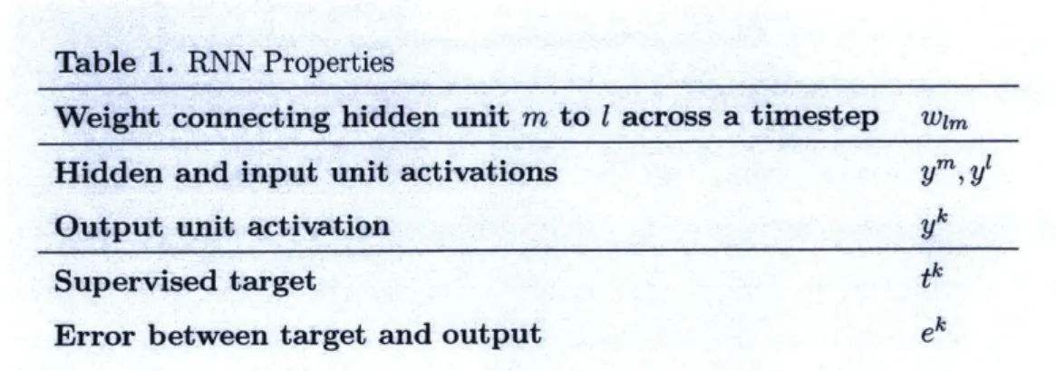
The network in Figure 9 gives a general understanding of how recurrence happens in RNNs. A more fundamental RNN than that of Figure 9 can be represented by taking the unit as a single perceptron, and the internal state of the unit as the activation of the unit itself. Using this more fundamental design of the RNN, the RNN learning algorithm here can be seen more clearly. Here, we present the integral equations of its learning algorithm. A more comprehensive derivation can be found at [Gers, 2016]. Table 3.2.1 shows the notation used for weights, activations and errors of the network.
Table 1. RNN Properties
Weight connecting hidden unit m to 1 across a timestep wim
Hidden and input unit activations yM, y
Output unit activation yk
Supervised target tk
The process of learning consists of a forward pass and a backward pass. In the forward pass, information is propagated from the input layer, through hidden layers, to the output layer, until the cost function E(t) is produced. In the backward pass, information is propagated from the cost backwards through the hidden layers of the network.
Forward Pass
Consider a unit in the network with activation y'. The activation of the unit is updated
at each timestep, and is computed by applying a differentiable function
f to the weighted
sum of inputs to the unit, net' (t) and net (t). The inputs to the unit consist of hidden unit activations from the previous timestep and external inputs from the current timestep.net' (t) = Wimyt (t - 1), (33)
where ym (t - 1) represent hidden unit activations.
netz(t) = Wimm(t) (34)
where ym (t) represent external inputs.
The sum of these inputs are then squeezed by f to generate y'(t).
y'(t) = f(net' (t) + net(t)). (35)
The updated hidden unit activations are then used to calculate the output unit activa-tions at the current timestep.
net'(t) = wk y (t) (36)
yk(t) =
fk(netk(t))
(37)
Using yk(t) and the supervised target values, tk(t), an error function, E(t) is calculated.
E(t) is then summed over all timesteps t, to produce a cost function, E. A simple
example of an error function is the squared error function (equation 39).
ek(t) = tk(t) - yk(t) (38) E(t) =
E ek
(t)2 (39) k E=
E(t) (40) t Backward PassAfter each computation of E(t), the derivative of E(t) with respect to the weights wlm is calculated [Pascanu et al., 2013],
aE(t) _ E E (t) aykt) yi(t) y(r) (41)
Owim k 1 O<r<t Oyk(t)
ay
1(t) ay,(r) awIm
OE E OE(t) (42)
awlm
t
When the derivatives for all timesteps, t, in the range [0, T] have been calculated, a gradient descent learning algorithm is applied to change each weight wim of the network. The weights are changed in the negative gradient direction to minimize the cost E, thereby producing yA in the next epoch that are closer in value to tk.
Awlm = -a awl (43)
where a is the learning rate of the network.
Vanishing Gradient Problem
The recurrence of the internal cell state in RNNs creates temporal memory that is used in the generation of outputs of the network. However, the temporal memory of RNNs can be limited if the weights wim and differentiable squeezing functions
f
fall withincertain bounds; these are called the vanishing-gradient bounds (as opposed to the ex-ploding gradient bounds), and they are specified in [Pascanu et al., 2013; Hochreiter and Schmidhuber, 1997]. This dependence of on wim and
f
can be clearly seen when the -yt term, from equation 38, is expanded out:0y(t) OyW(i) (44) ay(r) r<i<ty(i -
1)
= y 1) f(Z imYm(I 1) + y )) (45) aII y(i' - ZWm)mr<i<t
m
M'
=
f
f'Z wimym _ 1) + E WimY n(,) wIm (46)r<i<t m M'
The 22it term can be thought of as transporting the error, Ek(t) back in time to r,ayl (r)
where r < t [Pascanu et al., 2013]. The repeated multiplication of If'(EZ Wimy(i
-1) + E m' Wj/y '(I)) Em WimI < 1 for each time step i in the range r < i < t causes
the 2 to exponentially decrease with decreasing r (increased gap between r and t), rendering the influence of weights and activation values from early time steps (in the unrolled RNN) to be negligible in calculating the error for each weight, 9E(t), at the
current time step. This effect is called the vanishing gradient problem.
To overcome the vanishing gradient problem, the Long Short-Term Memory (LSTM) block, composed of LSTM cell(s), was constructed, to replace the units, composed of perceptron(s), widely used in MLPs.
3.2.2 Recurrence with Long Short-Term Memory Blocks
The premise for using Long Short-Term Memory blocks is to overcome the exponentially decreasing product that is generated through the repeated multiplication of the terms below (48) for each time step i in the range r < i t,
f'
Wimy m(i - 1) + WimYm(Z)>3
Wim. (47)A simple way to overcome this problem is to set the value of the terms equal to 1.0,
1 =f' Wimum(i - 1) + E wimYm() Wlm. (48)
Integrating the above equation yields,
y'(i) f (ZWmYm(i - 1) + ZwimYmW (49)
m m
I
~
w1MYMpz _ 1) + E WmYM(z)EM
Wim(z
Wim m( -1)Thus, the the hidden layer activation function
f is linear, simply scaling its input by a
constant. We can simplify equation 49 to make the relationship between the current-step unit y'(i) and previous-step units ym(i - 1) clearer, y'(i) = f (v(ym(i - 1))) (50) 1 = -v(ym (i - 1)) q
where v is a linear function of ym(i - 1), that sums the weighted current-step inputs
ym(i) and weighted previous-step units ym(i - 1), and = 1
is a scaling term. Setting the values of the terms (48) enforces constant error flow, and is implemented through the constant error carrousel in LSTM blocks [Hochreiter and Schmidhuber,
1997. The constant error carrousel (CEC) exists in the LSTM block as a cell state,1 2
that has a linear recurrence in time.
Similar to equation 50, the cell state sc(i) at the current time step is related the cell state at the previous time step sc(i - 1) by
sc(i) = lr(sc(i - 1)) (51)
1 2
The cell state is not to be confused with the internal unit state ht of perceptron-unit RNNs, from Section 3.2.1.
where the activation f = 1 is linear; and q is a linear function, which enforces
O,(Z) = 1
(52)
asc(i
- 1)Having updated the cell state, sc(i) influences the unit activation yl(i) produced at the current step as follows
y'(i, sc(i)) =A(i, q(sc(i)) (53)
= A(i, 7?(sc(i - 1, y'~ 1))))
where A is a non-linear function. The specific functions which A and q express are described in the Information Flow section below.
In LSTM unit networks, units refer to blocks, where each LSTM block contains one or more cells, and has gates on the outside that control the flow of information through the block. Figure 10 shows a traditional LSTM block, with a single cell. sc is the cell state of the
jth
unit. However, for consistency with the rest of this study, we transform the indices i,j
to 1, m when referring network units. The arrows pointing into the unit are the weighted collection of input sources at each time step, consisting of previous cell states sc(i - 1), external inputs ym(i), and previous unit activation ym(i - 1) [Graves],net' = PM( wpm(i -1) + ym(i ) + ym(i z ) (54)
where in comparison with the notation of Figure 10, net = net,1 (similarly, y = yPl)
and p = c, in, out; refers to the points of contact of the input sources with the block: direct contact, input-gate and output-gate.
Information Flow
The CEC of a LSTM unit enables the retention of memory acquired from all previous time steps. The error backflow through every activation besides that of the CEC either decays or grows exponentially, but the error backflow through the cell state remains constant. This is because, at each time step, information from the previous cell state is maintained
(without scaling) in the new cell state by a simple addition algorithm: s, = si + (Figure 10). Furthermore, from equation 55, we see how s, is the intermediary between the previous time step input y(i -- 1), and current time step output, yl(i).
In the forward pass, the following sequence of algorithms are implemented for information flow through the LSTM unit: First, input sources flow directly into the unit as
net'.
Second, a function g (Figure 11), squeezes the input sources,
g(netc).
Third, the input gate activation value multiplies with the squeezed input sources, deter-mining the percentage of input source information that passes into the cell state,
Yig(net4).
Fourth, the cell state updates itself by adding the squeezed and gate-multiplied input to the previous cell state,
s1 = s + y- g(net,).
Fifth, the updated cell state is then squeezed by the function h (Figure 11),
h(sl).
The last step, is multiplying the squeezed updated cell state with the output gate, which decides on the percentage of release of the squeezed cell state out of the memory block, as outputs
y1 = h(si) -y .
The sigmoid function,
f with range [0,1] (Figure 11) acts on net'n and net' to generate
yin and y . y1 and y are gated-activation values that control the percentage of
source input information that is added to sc at each time step and the percentage of
sc that is outputted at each time step respectively. This ensures that irrelevant source
inputs (i.e.: typically, weights wim are randomly initialized at time step t = 0 of the first training epoch, causing source inputs and network outputs at early time steps of the first training epoch, to be more random and non-representative of the data) have low
impact on weight-updates Awlm and network outputs y, at each time step. The idea of
using gates to control inputs that access and outputs that leave a linearly growing cell state, is addressed by Hochreiter and Schmidhuber [1997] as the solution to input weight
conflicts and output weight conflicts.
The LSTM unit introduced by them (Figure 10) is called the traditional LSTM block as the modern LSTM block uses another gate, called the forget gate, which is fed to the updated cell-state. The problem the forget gate solves is the saturation of h(sl) due to the linear-growth of s'. Thus, the forget gate serves to control the unbounded growth of the cell state, keeping s within regimes of non-zero gradient of the function h. Similar to the input and output gate, the forget gate is generated by multiplying input sources with the function
f
(Figure 11), and then multiplying the updated cell state for control[Gers, 20161.
netc,
se,=s
,+ g yIn yC'g
g
y'"n'
1h
h y*w'
Wei
Iy
fi Y outJ jIC 1Winji
net,
w
o Inetou
Figure 10: Long Short-Term Memory (LSTM) block. Diagram from [Hochreiter and
tr - ---.- ..-····-.. '.
--
-
~ I I ·•t j..
'..
,,..
..
, l g(x) I h(x) ., I ,,.
•··'
.,
.,I i'
.
.
... 1..
'
..
"!.. 4..
...
...
; ,;- ;:. ;; ;...
.,--~
...
... ... ...
.
..
.
..
..
..
..
..
X X.
:
f
~-
' ; .. t I ' "Iu
i
f(x) "f '..
,..
,
' 1:
:
r
' 1b
-
~
x' .; ;; ii -:. -~Figure 11: Functions used for information flow and control thro-qgh LSTM block. The function g squeezes input source$ directly entering the block, the function h squeezes the updated cell state, and the function
f
generates control with gated-activation values. Mathematically, these functions are different transformations of the logistic sigmoid:- 4 2 h- 2 1 d f - i

![Figure 4: Cross-sectional diagrams showing the range of East Antarctica. Figure from Schoof and Hewitt [2013].](https://thumb-eu.123doks.com/thumbv2/123doknet/14671344.556921/18.917.208.677.152.352/figure-sectional-diagrams-showing-antarctica-figure-schoof-hewitt.webp)
![Figure 10: Long Short-Term Memory (LSTM) block. Diagram from [Hochreiter and Schmidhuber, 1997].](https://thumb-eu.123doks.com/thumbv2/123doknet/14671344.556921/39.917.208.708.613.848/figure-long-short-term-memory-diagram-hochreiter-schmidhuber.webp)

