Cyclical Dynamics in Idiosyncratic Consumption
Risk
by
Allison Cole
B.A. Boston University (2013)
M.A. Boston University (2013)
Submitted to the Sloan School of Management
in partial fulfillment of the requirements for the degree of
Master of Science in Management Research
at the
MASSACHUSETTS INSTITUTE OF TECHNOLOGY
May 2020
c
○ Massachusetts Institute of Technology 2020. All rights reserved.
Author . . . .
Sloan School of Management
May 8, 2020
Certified by . . . .
Jonathan A. Parker
Robert C. Merton (1970) Professor of Finance
Thesis Supervisor
Accepted by . . . .
Catherine Tucker
Sloan Distinguished Professor of Management
Professor, Marketing
Faculty Chair, MIT Sloan PhD Program
Cyclical Dynamics in Idiosyncratic Consumption Risk
by
Allison Cole
Submitted to the Sloan School of Management on May 8, 2020, in partial fulfillment of the
requirements for the degree of
Master of Science in Management Research
Abstract
This paper examines cyclical dynamics of idiosyncratic consumption risk using consumption data from the Nielsen Consumer Panel and the Panel Study of Dynamic Income. With GMM estimates and supplemental graphical analysis, I show that the idiosyncratic risk in consumption is i) highly persistent, with an autocorrelation coefficient near unity ii) strongly countercyclical, with the conditional variance rising by an average of 25 percent from peak to trough. Compared to previous findings on income dynamics, I show that the variance of idiosyncratic consumption risk is also countercyclical, but less so. Moreover, I do not find that consumption risk displays procyclical skewness, as has been shown with income risk. Furthermore, in a simple asset-pricing framework, the estimated countercyclical cross-sectional variance of consumption raises the equity premium by 4.1 percent from the representative-agent case, using a risk aversion of only 10-15.
Thesis Supervisor: Jonathan A. Parker
Acknowledgments
I am grateful to my adviser, Jonathan Parker, for invaluable guidance and sup-port throughout this project. I also thank Hui Chen, Dan Greenwald, Eben Lazarus, Debbie Lucas, Christopher Palmer, Larry Schmidt, and Adrien Verdelhan for helpful comments and suggestions. Pierre Jaffard, Lu Liu, Yura Olshanskiy, Pari Sastry, and participants at the Sloan Finance Workshop also provided helpful discussions. This paper presents the researcher’s own analyses calculated (or derived) based in part on data from The Nielsen Company (US), LLC and marketing databases pro-vided through the Nielsen Datasets at the Kilts Center for Marketing Data Center at The University of Chicago Booth School of Business. The conclusions drawn from the Nielsen data are those of the researcher and do not reflect the views of Nielsen. Nielsen is not responsible for, had no role in, and was not involved in analyzing and preparing the results reported herein. All errors are my own.
I
Introduction
Consumption outcomes are the main object of interest for the design of tax and transfer policies, benefits from insurance, and the welfare cost of business cycles. Moreover, consumption risk plays a key role in the pricing of assets. Several facts have been documented regarding the income process, with various (and sometimes conflicting) conclusions. Namely, that there appear to be differences in both the variance and the skewness of the distribution of income outcomes during economic contractions versus expansions. These findings verify the very natural conclusion that during a recession, the probability of a large income drop increases, while the probability of a large income increase does not. What is not yet well understood however, is how these income dynamics translate to consumption.
The primary reason why income has been more commonly studied than con-sumption is that better administrative data is available for income. However, the ultimate object of interest is consumption. Consumers have utility over consump-tion, not income; we price assets using consumption risk, not income risk. While we can draw some implications about consumption using income, in a world where not all consumers are hand-to-mouth, the conclusions are incomplete. In this pa-per, I circumvent this issue by bringing the methods used to study income to a rich source of consumption data. I use the Nielsen Consumer Panel (CP) dataset, which tracks consumption expenditures at the household level. This dataset has several advantages over other measures of household consumption. First, it is much larger than most other commonly used consumption datasets such as the Panel Study of Dynamic Income (PSID) and the Consumer Expenditure Survey (CEX), with about 40,000-60,000 observations per year. In addition, the CP is not subject to the same measurement error as survey based measures because its relies on scanner data, rather than participant recall. To corroborate the results found in the CP, I repeat all anal-yses on the PSID and find similar results.
counteryclical. On average I find that the standard deviation rises by 25 percent from expansion to contraction. I also find that idiosyncratic consumption risk is highly persistent, with an annual autocorrelation coefficient close to unity. Moreover, I find no evidence that the the skewness of the persistent shock changes based on economic conditions, contrasting the results found for income, such as Guvenen, Ozkan and Song (2014). These results hold across both datasets, the CP and the PSID, as well as subsamples of the population that are more likely to be stockholders.
I begin the analysis by extending the parametric framework of Storesletten, Telmer and Yaron (2004b) (henceforth, STY). The key ingredient of this model is that it allows the variance of a persistent shock to income to vary based on the aggre-gate state of the economy. Following an extension developed by Busch and Ludwig (2018), I also assume that the skewness of the persistent shock is dependent on the aggregate state. The variance and skewness can be solved for in closed form and then estimated using the same Generalized Method of Moments (GMM) estimator devel-oped by STY. Moreover, I extend the framework in a way which allows me to control for inequality, hence the trend increase in inequality over time does not confound the results on cyclicality. Both graphically and with the GMM results, I show that the volatility of the persistent shock increases significantly as the economy moves from expansion to contraction. However, there is insufficient power and precision in my sample to show that the skewness changes. This confirms the original finding of coun-tercyclicality of STY, though I find a much smaller magnitude of councoun-tercyclicality in consumption than they did for income (a 25 percent increase from peak to trough versus a 75 percent increase). My dataset results in more precise estimation of the model’s parameters and higher power in failing to reject the model.
The basic identification strategy relies on the fact that the persistent shock ac-cumulates over the life-cycle such that the distribution of consumption observed for a given cohort widens as the cohort ages. The key is to take advantage of both year and cohort variation in consumption risk. As an example, suppose that we wish to examine the consumption outcomes of two groups of individuals aged 35. The first
group was born in 1955 and the second was born in 1970. Both are subject to id-iosyncratic consumption shocks, the variance of which is countercyclical. Hence, the former group should exhibit a larger within-group variance of consumption (at age 35, after conditioning on observables) because those born in 1955 have experienced more years of economic contractions than those born in 1975 (ie, there were more con-tractions from 1980-1990 than from 1995-2005). If consumption risk is systematically different between expansions and contractions, then the cohort variation will identify these differences. The same logic applies if we assume that the skewness varies across states as well.
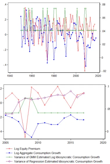
As a next step, I use the modeling framework to derive a simple asset pricing relation. By calculating the implied growth rate under the specified consumption process, I derive the economy’s stochastic discount factor. Then, I show that the risk premium is a function of the return’s covariance with aggregate growth and the return’s covariance with the variance of idiosyncratic components of consumption. As a result, this idiosyncratic risk amplifies the risk premium when its variance covaries negatively with the return. This is exactly what we would expect if the variance is in fact counteryclical. Indeed, I observe this in the data: on average, the correlation of the real return with the model-implied variance of the idiosyncratic component of consumption is -.41. Combined with a risk aversion of only 12, this increases the equity premium by 4.1 percent during the post-war period. Over my sample period, the importance of this finding is evident during the financial crisis: as stock returns fell sharply, the variance of idiosyncratic risk rose sharply, thus producing a high required expected return during the financial crisis.
The contribution of this paper is three-fold. First, I document previously un-known facts about the cyclicality of the consumption distribution in the CP. This dataset has been widely used in many fields of research from Industrial Organization to Household Finance, hence understanding more precisely trends in the data and how it compares to income is valuable. Second, I highlight several important ways in which the consumption risk appears to differ from income risk. Lastly, I demonstrate
how idiosyncratic risk can amplify the equity premium in a simple and commonly used framework for modeling shocks.
I.1
Related Literature
As mentioned above, the cyclicality of labor income risk has been extensively studied. STY conclude that idiosyncratic risk in labor income, is i) highly persistent, with an annual autocorrelation coefficient of approximately .95 ii) highly countercycli-cal, with a conditional standard deviation that increases by approximately 75 percent when the macroeconomy moves from contraction to expansion. Guvenen, Ozkan and Song (2014) refute this result, finding that the variance is not counteryclical but the the skewness is strongly procyclical. Busch and Ludwig (2019 WP) find that the vari-ance is countercyclical and the skewness is procyclical. Krebs (2007) shows that job displacement risk (and hence income risk) has a large welfare cost. Schmidt (2016) shows that idiosyncratic labor risk in the tail is key driver of asset prices.
Many papers have also studied consumption risk. In a separate paper, Storeslet-ten, Telmer, and Yaron (2004a) use PSID and Consumer Expenditure Survey (CEX) data to show that shocks to both income and consumption are highly persistent over the lifecycle. Gourinchas and Parker (2002) also document strong lifecycle dynam-ics in consumption using the CEX. Attanasio and Davis (1996) show the failure of consumption insurance and that there is large variation across groups based on edu-cation. Parker (2001) finds that medium-term consumption risk can in part explain the equity premium. Cogley (2002) constructs an equilibrium factor model based on consumption data from the CEX. While he documents the cross-sectional variation in consumption risk, the model finds that it does poorly in explaining the equity pre-mium. Constantinides and Ghosh (2017) show that shocks to household consumption growth are negatively skewed, persistent, countercyclical, and drive asset prices. De-spite the vast literature, an analogous study to STY or Guvenen, Ozkan and Song (2014) using complete consumption data, or any study of idiosyncratic consumption
risk using the CP, has yet to be completed to the best of my knowledge1.
This paper also contributes to the literature on consumption based asset pricing. Lucas (1994) shows that most idiosyncratic risk can be smoothed away via securities transactions. However, this assumes that all individuals are participating in such markets. Constantinides and Duffie (1996) suggest a model with labor income shocks and show that idiosyncratic risk lowers the risk free rate due to the precautionary sav-ing effect. Heaton and Lucas (1996) study a model of idiosyncratic labor shocks with transactions costs and find that the direct effect of transactions costs on the ability to self-insure against these shocks can explain a significant proportion of the equity pre-mium. Guvenen (2009) provides a model with both idiosyncratic labor-income risk and limited participation, showing that stockholders must be highly compensated for the risk they take when insuring against labor income shocks, which can explain the large equity premium. Duffee (2005) shows that consumption risk is priced and that consumption growth is closely tied to stock returns. Di Maggio, Kermani and Majlesi (2018) use administrative data from Sweden to document that household consump-tion responds strongly to stock returns, particularly at the lower end of the income distribution.
II
Data
II.1
Nielsen Consumer Panel Data
The data underlying my estimation are from the Nielsen Consumer Panel (hence-forth, CP). The CP is a longitudinal panel of approximately 40,000-60,000 households per year in the United States, members of which continually provide information to Nielsen about their household characteristics and purchases. Nielsen samples 48 states and their major markets and panelists are geographically dispersed and
demograph-1STY do replicate their analysis on food consumption, which is available in the PSID. They find
ically balanced. The data are available from 2004-2017 and the panel has steadily grown in size since 2004. The panel is unbalanced with some panelists staying in the sample for several years and others joining or dropping out in any given year. The CP is rich in demographic information including household size, age, education, race, occupation, income, and location. Demographic data on household members are collected at the time of entry into the panel, and are then updated annually through a written survey that takes place during the fourth quarter. Nielsen provides sam-ple weights to make the samsam-ple representative of the U.S. population. I apply these weights in all of the analyses.
To record purchases, the Homescan panelists are given in-home scanners. Pur-chases include food and non-food items. The purchase information in the data in-cludes the date of the trip, the retailer, the retailer’s zip code, and total dollars spent. To get total consumption, I simply sum up the amount spent on all trips in a given household for the entire year. Note that because the CP only measures pur-chased products at the stores included by Nielsen, this measure of consumption does not account for services such as housing and utilities, health care, financial services, and most durable goods. This point bears more discussion, and I will return to it momentarily.
Nielsen offers the panelists a variety of incentives to join and remain in the panel. Some examples are monthly prize drawings, gift cards, and sweepstakes. Nielsen filters out households based on purchasing thresholds in order to remove households that are not active and may bias the results. My analysis includes only actively reporting households who have a least one trip per month over each year.2
There are several issues that arise when working with longitudinal data. Because the panel is unbalanced, limiting the analysis to only those who remain in the panel for the entire period would lead to a relatively small sample size. Additionally, such a panel would be subject to survivorship bias. Most problematic for the approach in this
2I refer interested readers to Kaplan and Menzio (2015), Broda and Weinstein (2010), and Broda
paper is that a longitudinal panel inherently features an average age that increases with time. Because the approach relies on variation in experience across household with macroeconomic conditions, this is problematic. As in STY, in order to avoid these issues I construct sequences of overlapping three-year subpanels consisting of households who remained in the sample for three consecutive years. This results in panels with a relatively stable average age as well as similar education and income characteristics. Table I shows summary statistics by year, while Table II shows the summary statistics for each subpanel. Overall, the average age and median income levels are slightly more stable for the subpanels, as desired.3 I also drop cohorts with fewer than 1,000 observations in order to ensure that I have sufficient sample size within each cohort.
There are a few other selection criteria with which I limit the analysis. First, the head of the household must be aged between 25 and 60.4 Additionally, they
must have non-missing consumption, race, education, family size, and income data in order to be included. Table IV shows the summary statistics for the entire period relative to the Survey of Consumer Finance (SCF). As one can see by comparing columns two and three of Table IV, these restrictions do lead to some differences in the estimation sample versus the full sample. Participants in the estimation sample are on average younger, more college educated, and have higher income. While this may introduce some bias in the estimation, it is a necessary step for identification. Moreover, we know from the limited participation literature that wealthier, higher educated individuals are more likely to own stocks and thus this sample is exactly the relevant one when it comes to asset pricing implications.5
There is substantial evidence to support that the CP is a reliable source of con-sumption data. Returning to Table IV, one can see that Nielsen compares quite favorably to the SCF. The median income, mean age, and percentage of college
ed-3Note that the increasing age problem is less of an issue here than it was in STY, given the
shorter range of the panel.
4When indicated, I further limit this to age 30-55. 5See for example Mankiw and Zeldes (1991).
ucated levels are similar. This is reassuring that the Nielsen data is a representative sample.6,7. Moreover, Einav, Leibtag and Nevo (2008) run a validation study of the
CP by comparing the purchase data recorded by consumers to data recorded by the retailer. The most problematic field is the price variable. They show that errors are primarily due to two reasons: 1) standard inputting errors by panelists 2) Nielsen’s imputation of prices using store averages. However, since I am primarily interested in cyclicality, any measurement error in the data should not affect my estimates as long as the errors do not vary over the business cycle.
Above, I raised the issue that the CP comprises primarily non-durable good con-sumption and does not include services or durable goods. This may raise concerns that it is difficult to make statements about cyclicality and asset prices without hav-ing a complete picture of consumption. Regardhav-ing cyclicality, however, havhav-ing an estimate of non-durable consumption can only understate the true cyclicality in the data, as non-durable consumption is less cyclical than durable consumption. There is much empirical evidence to support this. For example, Berger and Vavra (2015) find that consumers adjust different types of consumption cyclically, particularly that durables are more sluggish to respond to shocks during recessions due to microeco-nomic frictions. Kaplan, Mitman and Violante (2016) show that the CP data can be used to replicate the qualitative results from Mian, Rao and Sufi (2013) who use housing supply elasticity as an instrument to measure the effect of the housing bust on household consumption. The Mian, Rao and Sufi (2013) analysis relies on automobile spending as a proxy for consumption. The fact that Kaplan, Mitman, and Violante (2016) are able to find similar results using the CP, which contains only information on non-durables, is reassuring.
As a further check on the validity of the CP data, I have completed a quick back of the envelope exercise to put the data in perspective. As of 2010, services
6While the mean income is much higher in the SCF, it is known that the SCF oversamples wealthy
individuals, see for example Campbell (2006)
7The CP does not contain information about stock ownership. The estimates presented in this
table are based on a probit model of stock ownership fitted from the PSID. I defer further discussion of this until Section 4.4.
made up approximately two-thirds of total expenditures in the CEX and the PCE.8. Moreover, durables make up about third of all goods consumption (about one-ninth of total consumption). So, in the CP, we expect to observe only about 20 percent of what we think of as true consumption. Indeed, the Bureau of Economic Analysis (BEA) estimates per capital PCE to be 63,563 dollars in 2010, implying about 12,000-13,000 dollars in consumption of non-durable goods.9. My sample has
an average consumption of approximately 4,500 dollars over all the years, indicating that the CP is capturing only one-third of what we would expect. This is reasonable coverage given that we can’t be certain that all members of the panel scan every purchase and that not all goods are covered by the Nielsen scanner system, as well as general measurement error.
One might also worry that the distribution of durables versus non-durable con-sumption is heterogeneous across income. As a result, my concon-sumption estimates could be biased differently for those in different income groups. Based on the CEX, there is some evidence that the share of durables of total consumption is increasing in income (see Table V). Taking these moments from the 2010 CEX literally, one would conclude that the CP is missing 65 percent of consumption for those with an income between 50,000-69,999 dollars, but missing 70 percent of consumption for those with an income greater than 70,000 dollars. One can imagine an adjustment of the data that accounts for this, however that is beyond the scope of this paper. To alleviate concerns about this, I again make the point that durables are in fact more cyclical than non-durables. Hence, anything that I measure here represents a lower bound on the true implications of cyclicality for consumption. This may be even more relevant for those in higher income brackets. What is observed in the CP is interesting for the very fact that it represents items that are likely to be the last things to be cut in the face of recessions, such as a groceries and health and beauty products purchased at a drugstore.
8https://fred.stlouisfed.org/release/tables?rid=53&eid=43861&od=2010-01-01#
https://www.bls.gov/news.release/cesan.nr0.htm
9
With regards to the asset pricing implications, the lack of information about durables may still be cause for concern. There is some evidence, such as Yogo (2006), that durable consumption is highly correlated with asset prices. However, this frame-work relies on extremely high risk aversion and non-separability of utility and thus may not be generalizable. Other evidence, such as Dunn and Singleton (1986), Eichen-baum and Hansen (1990), and Heaton (1993, 1995) consider the consumption Euler equation when utility depends on services from consumer durables. They show that adding consumer durables does not help explain the level of the equity premium. Piazezzi, Schneider and Tuzel (2007) develop a model that introduces ”composition risk", that is the share of housing as total consumption, and that this risk induces low frequency movements in stock prices that are not driven by news about cash flows. Together, these pieces of evidence are mixed on the relevance of non-durable consump-tion for asset prices. Moreover, the standard in asset pricing is to use non-durable consumption, starting with Mehra and Prescott (1985). Applying the methodology used in this paper to a consumption data with more complete consumption is an in-teresting area for future work. The present paper aims to draw conclusions based on the best sources of consumption data that are publicly available. There is ample ev-idence to support that durable consumption and non-durable consumption co-move strongly10, and thus there is still something to learn from looking at the available non-durable consumption.
II.2
The Panel Study of Dynamic Income
I supplement my analysis using data from the Panel Study of Dynamic Income (henceforth PSID) from 1999-2017 (biannually). This was the source of data for STY, however they used income data from 1968-1993. Each household in the PSID is interviewed annually from 1968-1997 and biannually after that. Sample sizes began at around 5,000, 3,000 of which were representative of the U.S. population and 2,000
were a low-income over sample. Households are asked detailed questions about their demographics, income, and spending, among other things.11
The PSID also contained food consumption data from 1968-1993. However, since 1999, the PSID has added more detailed consumption categories in an attempt to match the CEX. As such, I can use this data as another source of semi-complete household consumption data. In theory, the PSID should also contain information about durable and service spending, thus bypassing the issues discussed with the CP. However, the sample size is much smaller, thus limiting the power of inference.
I make the same restrictions on the PSID data as with the CP. That is, I construct subpanels in which the household must appear in two-consecutive (biannual) surveys. Moreover, the household must have non-missing education, consumption, and income data and must be of working age. Summary statistics for the PSID are shown in Table III. As expected, consumption in the PSID is much higher than in the CP. Table IV also shows how the PSID compares to the CP and the SCF. Overall, the PSID sample is younger, less white, less educated, and slightly lower-income.
II.3
Macroeconomic Data
I use four sources of macroeconomic data to classify years as expansions and contractions. The first uses the NBER business cycles. These are derived from the monthly NBER definitions of contractions and expansions. I convert the monthly definitions to yearly ones by classifying a year as contractionary if it has at least six months considered to be contractions. If contractions spanned more than six months over two calendar years, I designate the first year as contractionary. This results in a total of nine contractionary years from 196912-2017. Appendix Table A1 shows how each year is classified using the different definitions. The shaded years in Figure II
11I refer readers to Blundell, Pistaferri, and Preston (2008) for a more detailed discussion of the
PSID
indicate NBER recession years.
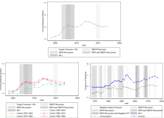
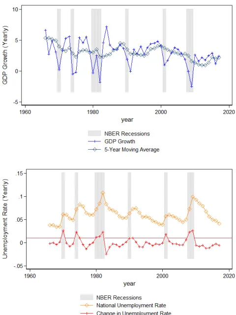
The second definition is real GDP growth from the National Income and Product Accounts (NIPA), maintained by the BEA. Using a similar definition as STY, I classify a year as a contraction if the growth is below the mean growth within the past five years an expansion if growth is above the mean growth for the past five years. This results in a total of 18 contractionary years over the same time period, hence this definition is more sensitive. The top left figure of Figure II shows GDP growth over time compared to the the five-year moving average.
The third definition uses unemployment data from the Bureau of Labor Statistics (BLS). I classify a year as a contraction if the national unemployment rate increases by more than one percent. This results in eight contractionary years over the same period. The top right figure of Figure II shows the unemployment rate over time.
Lastly, I use stock returns from CRSP. I calculate the equity premium by sub-tracting the annualized 30-day T-bill return from the annual market return. I then classify a year as a contractionary if the real return is less than five percent. This results in 16 contractionary years over the same period. The bottom figure of Figure II shows the excess return over time.
Table VI shows the correlation matrix for each measure of contractions. They are all positively correlated, with the NBER indicators and the unemployment indicators being particularly similar, with a correlation of .93. The equity premium indicator is the least similar to the other series. This becomes relevant when discussing the results. My findings are robust to each of these definitions, however they are stronger or weaker depending on the definition used.
III
Estimation Approach
III.1
The Consumption Process
Following STY, I estimate the same time-series model for idiosyncratic risk, but for consumption rather than income.13 This model has two key ingredients that make it ideal for the questions at hand. First, it accounts for the deterministic component of consumption that is not affected by idiosyncratic risk. Second, it allows for the moments of the distribution of shocks to change depending on the aggregate state of the economy. A third component that I add by extending upon the original framework, is controlling for inequality; this will be discussed below with assumption A.4. These three things together allow me to use this model to precisely estimate how cyclicality affects idiosyncratic consumption risk.
The first step is to decompose consumption into its observable components, time component, and an unexplained, or idiosyncratic component. Denote 𝑐ℎ𝑖𝑡 as the loga-rithm of consumption for household 𝑖 of age ℎ at time 𝑡. Log consumption is specified as: 𝑐ℎ𝑖,𝑡 = 𝜃0+ 𝜃1𝑇𝐷(𝑌𝑡) + 𝜃𝑇2𝑥 ℎ 𝑖,𝑡+ 𝑢 ℎ 𝑖𝑡 (1)
where 𝐷(𝑌𝑡) is a vector of year dummy variables for 𝑡 = 2004, ..., 2017 and 𝑥ℎ𝑖𝑡 is a
vector of observable household characteristics. STY included the age of the male head of the household (plus age-squared and age-cubed), family size, and education level for the male head of the household in 𝑥ℎ𝑖𝑡. I also add race dummies and region-code dummies. The specification thus accounts for both aggregate variation in consump-tion and household observables. The main object of interest is the residual, 𝑢ℎ𝑖𝑡, which represents the random component of a household’s consumption that is idiosyncratic to that household specifically. I specify that 𝑢ℎ𝑖𝑡 follows a stochastic process, which is
13Similar models have been used in many other settings, such as Guvenen, Ozkan and Song (2014),
ARMA(1,1) and has regime-switching conditional moments:
𝑢ℎ𝑖𝑡= 𝛼𝑖+ 𝑧𝑖,𝑡ℎ + 𝜖ℎ𝑖𝑡 (2)
𝑧ℎ𝑖𝑡= 𝜌𝑧𝑖𝑡−1ℎ−1+ 𝜂𝑖𝑡ℎ (3)
with 𝛼𝑖 ∼𝑖𝑖𝑑 𝐹𝛼, 𝜖ℎ𝑖𝑡∼𝑖𝑖𝑑 𝐹𝜖, 𝜂ℎ𝑖𝑡∼𝑖𝑖𝑑 𝐹𝜂(𝑠𝑡), 𝑧𝑖𝑡0 = 0, ∀𝑖, 𝑡.14,15 The conditional variance
of 𝜂ℎ𝑖𝑡 is dependent on the aggregate state:
𝜇2𝜂 = ⎧ ⎪ ⎨ ⎪ ⎩ 𝜇2 𝜂,𝐸 if t is a year of expansion 𝜇2 𝜂,𝐶 if t is a year of contraction (4)
I extend the original STY model by also allowing the conditional skewness16 of 𝜂ℎ 𝑖𝑡 to
be dependent on the aggregate state:
𝜇3𝜂 = ⎧ ⎪ ⎨ ⎪ ⎩ 𝜇3𝜂,𝐸 if t is a year of expansion 𝜇3𝜂,𝐶 if t is a year of contraction (5)
The variables 𝑧𝑖𝑡ℎ and 𝜖ℎ𝑖𝑡 are the persistent and transitory shocks, respectively. 𝛼𝑖 is
a “fixed-effect" in the form of a shock at birth that is retained throughout life. Each component of the model serves a specific function. The fixed effects and transitory shocks allow us to better measure the primary objects of interest - 𝜇𝑘
𝜂 and 𝜌. The way
parameters will be identified involves examining how the cross-sectional moments of 𝑢ℎ
𝑖𝑡 change with age. However, much of the variation is common to households of all
ages. Hence, if there were no fixed effect, the magnitude of 𝜇𝑘𝜂 would be overstated, therefore overestimating the amount of idiosyncratic risk that households face. Like-wise, the transitory shock 𝜖ℎ𝑖𝑡 is included to capture measurement error.
14In the original STY paper, normality was also imposed on the distribution of 𝛼
𝑖, 𝜖ℎ𝑖𝑡 and 𝜂 ℎ 𝑖𝑡. I
relax that in order to estimate higher order moments; this will be discussed further in section 3.2
15In what follows, 𝜇𝑥
𝑦 represents the 𝑥𝑡ℎ moment of parameter 𝑦.
16Note that the model does not rule out regime switching for moments higher than the third.
In this paper, I focus only on the second and third moment, but it is possible that higher order moments are regime switching as well.
The i.i.d. assumptions imply that 𝛼𝑖 is not correlated with residual consumption
nor the persistent or transitory shock. This is a strong assumption. To understand this, note that it rules out the possibility that 𝛼𝑖 is time varying or that later-in-life
realizations of shocks could affect it. For example, this means that the fixed effect received at birth is drawn from the same distribution for everyone, regardless of when they are born. In other words, it assumes that there are no changes in inequality over time. However, this assumption, as well as the initial condition that 𝑧𝑖𝑡0 = 0, are essential to the estimation approach. These conditions allow us to interpret (2) and (3) as a collection of finite processes and thus we can condition on age. I now move on to discuss these assumptions in more detail.
Discussion of assumptions
As with any parametric estimation, the model requires some assumptions in order to provide structure. In this section, I’ll provide a brief discussion of the key assumptions underlying the estimation.
A.1 Functional form of the aggregate and the deterministic component
As shown in equation (1) The aggregate component is modeled using year dum-mies. The deterministic component is:
𝑓 (𝑥ℎ𝑖𝑡) = ˆ𝛽[1, ℎ, ℎ2, ℎ3, 𝑒𝑑𝑢𝑐𝑎𝑡𝑖𝑜𝑛𝑖𝑡, 𝑓 𝑎𝑚𝑖𝑙𝑦𝑠𝑖𝑧𝑒𝑖𝑡, 𝑟𝑒𝑔𝑖𝑜𝑛𝑖𝑡] + 𝜀 (6)
This specification of the aggregate and deterministic components is essential for identifying the residual, but beyond that it is not central. One potential issue that could arise out of this specification is that the deterministic component is invariant across time and individuals. This may inflate the residual, as we know that individuals from different socioeconomic backgrounds may have different deterministic profiles and that the profile may change over time17. Moreover,
modeling education as a deterministic component likely results in underestimat-ing the overall risk that agents face. However, estimatunderestimat-ing schoolunderestimat-ing decisions is beyond the scope of this paper. That being said, this specification is stan-dard in the earnings literature (Hubbard, Skinner and Zeldes (1994)). As a robustness check, I estimate the model on different subsets of the population based on education, income, and time period in Appendix Tables A4, A5, and A6, respectively. Some of the coefficients are significantly different from each other, particularly the race coefficients in the education and income regressions. The regressions split by time period also exhibit quite a bit of dispersion across the race and age coefficients. However, the order of magnitude and direction of each coefficient is preserved across each specification. More importantly, the concavity in age is maintained among each of the samples. In section 4.2, I will show how the results of my first-stage estimation compare to others in the lit-erature; the results are reassuring. Moreover, I will show in section 4.4 that my findings are robust to using specific subsets of the population based on income and education.
A.2 Functional form of the residual
The residual, shown in equation (2) is modeled a a function of a fixed effect, a persistent shock, and a transitory shock. This is, again, standard in the literature and there is ample empirical evidence to support its validity (Abowd and Card (1989), Hubbard, Skinner and Zeldes (1994), Heaton and Lucas (1996) Blundell, Pistaferri, and Preston (2008), Guvenen, Ozkan, and Song (2014), and Schmidt (2016)).
A.3 The fixed effect 𝛼𝑖 is time invariant, drawn once at birth, and i.i.d.
This is a more substantial assumption, as it rules out time variation in 𝛼𝑖 and
dependence between 𝛼𝑖, for a given 𝑖, and subsequent realizations of 𝑧𝑖𝑡 and 𝜖ℎ𝑖𝑡.
In other words, the fixed effect is drawn from the same distribution for everyone, regardless of the year of birth. This rules out an increase in inequality (due to the fixed effect) over time. Time invariance in 𝛼𝑖 is actually not essential, but it
being uncorrelated with subsequent realizations of the other shocks is. Imposing time invariance is the most straightforward and tractable way of achieving this. The payoffs for making this assumption, along with assumption 4, which I discuss next, are large: they me to interpret the process for 𝑧ℎ
𝑖𝑡 in equation (3)
as a collection of finite processes, and thus condition on age. A.4 The persistent component follows an AR(1) process
∙ The initial condition: 𝑧0
𝑖𝑡 = 0 ∀ 𝑖, 𝑡
∙ The innovations 𝜂ℎ
𝑖𝑡 are i.i.d.
∙ The second and third moments of the AR(1) innovations are regime switch-ing
The assumption that 𝑧0
𝑖𝑡 = 0 for all 𝑖 and 𝑡 is perhaps the strongest assumption
imposed. However, it is very important for the estimation strategy: if 𝑧𝑖𝑡0 varied across individuals then I would not be able to identify the parameters of interest in equation (3). In light of more recent empirical evidence of rising inequality, there is reason to believe that this assumption may bias my estimates.18.
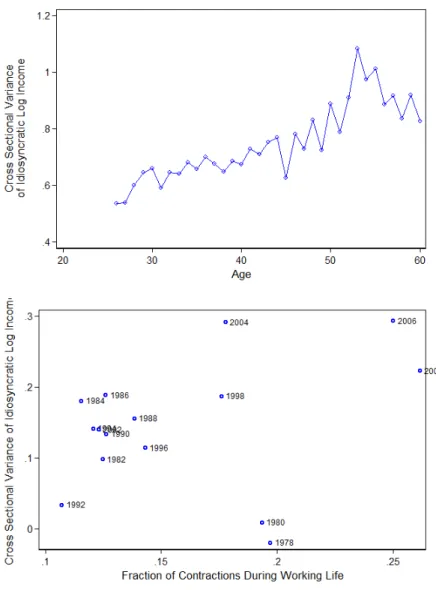
In-deed, looking at Figure I, one can clearly see that the residual variance of both consumption and income has increased over time.19 Even just in the period
from 2004-2017 of the CP data, it has increased by about 75 percent on av-erage. In the PSID, it has almost doubled since 1968. This means that it is difficult to disentangle the effects of business cycles and inequality. For example, consider two groups of 30-year olds. One enters the workforce in 1980 and the other in 2007. Looking at Appendix Table A1, one can see that both face three contractions of GDP growth in their first five years of working (between ages 25-30). Taking the model literally, this would imply that they should exhibit, on average, the same cross-sectional variance (and skewness) at age 30 (in 1985 and 2012, respectively). However, if one believes that inequality has increased
18See Blundell, Pistaferri, and Preston (2008), Aguiar and Bils (2015), Carrol, Tokuoka, and
White (2017), and Patterson (2018)
19These figures present only raw data, so some of the increase may also be due to change in the
from 1980-2012, then this may not be the case. Again looking at Figure I, we can see that residual variance has increased over time even when controlling for cohort. As a result, when observing higher variance among younger cohorts, it is possible to falsely attribute this to cyclicality when it may truly be driven by inequality.
However, there is a way to maintain this assumption while still accounting for the fact that the initial distribution of shocks has likely changed over time. I do so by controlling for the initial residual variance of consumption in the year that a cohort enters the workforce using food consumption data in the PSID going back to 1968. To achieve this, I add the initial residual variance of food consumption in year zero to 𝑥ℎ𝑖𝑡 in equation (1).20,21,22 While using only food consumption likely understates the true variance of consumption, it is the best proxy available going back far enough to provide controls for the oldest individuals in my sample.23 Adding this control, we can still assume that 𝑧0
𝑖𝑡 = 0
for all 𝑖 and 𝑡, but it should now be thought of as the initial shock net of the observed initial dispersion, which is plausibly unchanging over time.24 To see
this, recall that 𝑢ℎ𝑖𝑡 in equation (1) represents the idiosyncratic, or unobserved component of log consumption. I specify that it follows an ARMA (1,1) process:
𝑢ℎ𝑖𝑡 = 𝛼𝑖+ 𝜌𝑧𝑖𝑡−1ℎ−1+ 𝜂 ℎ 𝑖𝑡+ 𝜖 ℎ 𝑖𝑡 (7) = 𝛼𝑖+ 𝜌ℎ𝑧𝑖𝑡−ℎ0 + ℎ−1 ∑︁ 𝑘=0 𝜌𝑘𝜂𝑖𝑡−𝑘ℎ−𝑘 + 𝜖ℎ𝑖𝑡 (8)
20That is, I control for the orange line in the bottom panel of Figure I
21Note that adding this control does not substantially change the results of the first stage
regres-sion. The first stage regression results without the control are shown in Appendix Table (A3).
22In an alternative specification, I also run this regression controlling for both the variance and the
skewness of initial food consumption. The coefficient on skewness is not significantly different from zero and makes no difference in the estimation results using the residuals. Using a larger dataset than the PSID, in which skewness is more precisely estimated, would be a natural next step, were such a dataset available going back to the 1960s.
23I also repeat the analysis using the variance of income in the PSID as a control and the results
are similar.
24This is difficult to test as I observe very few individuals at age 25, when the initial variance should
be the same across all cohorts, conditional on the current state of the economy, if this assumption is valid. In Appendix A, I compare the initial residual variances for the cohorts that I do observe in year 0 and show that they are similar.
Hence, for somebody in their first year of the workforce, the residual is:
𝑢1𝑖𝑡= 𝛼𝑖+ 𝜌𝑧𝑖𝑡−10 + 𝜂𝑖𝑡1 + 𝜖1𝑖𝑡 (9)
Note that the fixed effect, 𝛼𝑖, the transitory shock, 𝜖ℎ𝑖𝑡, and the AR(1) innovation,
𝜂ℎ𝑖𝑡, are drawn from the same distribution for everyone. Thus, when aggregating across cohorts, the sum of these components is the same on average. Hence if there is variation in 𝑢1𝑖𝑡 across cohorts, as observed in Figure I, it must be the case that 𝑧0
𝑖𝑡 is not the same across cohorts. Moreover, 𝑧𝑖𝑡0 represents the initial
starting point of the permanent shock. We do not know exactly what determines this starting point, but it is specified to be unobservable. However, we can in fact observe something about where cohorts start off - i.e. the level and variance of their residual consumption or income when they enter the workforce. Hence, adding this control moves a portion of the determining factors of 𝑧𝑖𝑡0 from the unobservable part of equation (1) to the observable part.25
On the regime switching moments, this is simply a way to add structure to the model and identify cyclical effects. While this is a simplification for the sake of tractability, it is a useful starting point.26
A.5 The transitory component, 𝜖ℎ
𝑖𝑡, is i.i.d.
Again, this is a standard assumption that provides tractability.
III.2
GMM
I follow the same approach as STY in estimation. First, I run the regression in equation (1) to obtain residuals. The second step fits the stochastic process (2) to the cross-sectional moments of the distribution of residual log consumption. The system
25An alternative route would be to estimate 𝑧0
𝑖𝑡as a free parameter. This is an interesting avenue
for future research, but beyond the scope of the current paper.
26One can imagine a model with moments that are continuous, rather than binary, and scale
proportionally to the severity of the contraction/expansion. This is an interesting avenue for future work, but beyond the scope of the current paper
in (2) and (3) implies the following moments of this distribution27: Variance: 𝜇2(𝑢ℎ𝑖𝑡; 𝜃) = 𝜇2𝛼+ 𝜇2𝜖 + ℎ−1 ∑︁ 𝑗=0 𝜌2𝑗𝜇2𝜂(𝑠𝑡−𝑗) (10a) Covariance: 𝜇11(𝑢ℎ𝑖𝑡, 𝑢ℎ+1𝑖𝑡+1; 𝜃) = 𝜇2𝛼+ 𝜌 ℎ−1 ∑︁ 𝑗=0 𝜌2𝑗𝜇2𝜂(𝑠𝑡−𝑗) (10b) Skewness: 𝜇3(𝑢ℎ𝑖𝑡; 𝜃) = 𝜇3𝛼+ 𝜇3𝜖 + ℎ−1 ∑︁ 𝑗=0 𝜌3𝑗𝜇3𝜂(𝑠𝑡−𝑗) (10c) Coskewness: 𝜇21(𝑢ℎ𝑖𝑡, 𝑢ℎ+1𝑖𝑡+1; 𝜃) = 𝜇3𝛼+ 𝜌 ℎ−1 ∑︁ 𝑗=0 𝜌3𝑗𝜇3𝜂(𝑠𝑡−𝑗) (10d) where 𝜃 = (𝜌, 𝜇2𝛼, 𝜇2
𝜖, 𝜇2𝜂,𝐸, 𝜇2𝜂,𝐶, 𝜇3𝛼, 𝜇3𝜖, 𝜇3𝜂,𝐸, 𝜇3𝜂,𝐶) is the vector collecting all of the
parameters to be estimated. 𝜇2(𝑢ℎ
𝑖𝑡; 𝜃) and 𝜇3(𝑢ℎ𝑖𝑡; 𝜃) denote the second and third
central moment; 𝜇11(𝑢ℎ 𝑖𝑡, 𝑢
ℎ+1
𝑖𝑡+1; 𝜃) and 𝜇21(𝑢ℎ𝑖𝑡, 𝑢 ℎ+1
𝑖𝑡+1; 𝜃) denote the covariance and a
measure of co-skewness between 𝑢ℎ
𝑖𝑡 and 𝑢 ℎ+1
𝑖𝑡+1. The covariance and coskewness terms
enable me to separately identify the moments of the fixed effect 𝛼𝑖 and the transitory
shock 𝜖ℎ 𝑖𝑡.
As described in the previous section, the conditional second and third moments of the AR(1) innovation, 𝜂𝑖𝑡ℎ, are allowed to be state dependent. The aggregate state can either be an expansion or a contraction, and the variance (skewness) takes on a separate value in each state. Define an indicator variable 1𝑠(𝑡)=𝐸 = 1 if the economy
is an an expansion (denoted by E) at time 𝑡. Then we have:
𝜇2𝜂(𝑠(𝑡)) =1𝑠(𝑡)=𝐸𝜇2𝜂,𝐸+ (1 −1𝑠(𝑡)=𝐸)𝜇2𝜂,𝐶 (11)
𝜇3𝜂(𝑠(𝑡)) =1𝑠(𝑡)=𝐸𝜇3𝜂,𝐸+ (1 −1𝑠(𝑡)=𝐸)𝜇3𝜂,𝐶 (12)
In order to ensure that the central moments are precisely estimated, I collapse each observation into a five-year age groups, beginning at age 22. Hence, I have eight total age groups, denoted by ℎ𝑔: 22-26, 27-31, 32-36, 37-41, 42-46, 47-51, 52-56,
61.28. This results in an average of 3,990 observations in each age by year cell. I can thus calculate the empirical moments :
𝜇𝑘(𝑢ℎ𝑔 𝑖𝑡) = 1 𝑁ℎ𝑔𝑡 ∑︁ ℎ∈ℎ𝑔 (𝜇𝑘(𝑢ℎ𝑖𝑡)) for 𝑘 ∈ (2, 11, 3, 12) (13)
This represents the mean of the given moment (variance, covariance, skewness, or co-skewness) within an age group, ℎ𝑔, at time 𝑡. The theoretical counterpart is:
𝜇𝑘(𝑢ℎ𝑔 𝑖𝑡 ; 𝜃) = 1 𝑁ℎ𝑔𝑡 ∑︁ ℎ∈ℎ𝑔 𝑁ℎ𝑔𝑡(𝜇 𝑘(𝑢ℎ 𝑖𝑡; 𝜃)) for 𝑘 ∈ (2, 11, 3, 12) (14)
for a specific combination of the parameters, 𝜃. And so the moment conditions are
𝐸[𝜇2(𝑢ℎ𝑔 𝑖𝑡) − 𝜇 2(𝑢ℎ𝑔 𝑖𝑡 ; 𝜃)] = 0 (15a) 𝐸[𝜇11(𝑢ℎ𝑔 𝑖𝑡 ) − 𝜇 11 (𝑢ℎ𝑔 𝑖𝑡 ; 𝜃)] = 0 (15b) 𝐸[𝜇3(𝑢ℎ𝑔 𝑖𝑡) − 𝜇 3 (𝑢ℎ𝑔 𝑖𝑡 ; 𝜃)] = 0 (15c) 𝐸[𝜇21(𝑢ℎ𝑔 𝑖𝑡 ) − 𝜇 21 (𝑢ℎ𝑔 𝑖𝑡 ; 𝜃)] = 0 (15d)
for each year 𝑡 and age group ℎ𝑔. All in all, I have ℎ𝑔 × 𝑡 cross-sectional measures
of variance and skewness and ℎ𝑔× (𝑡 − 1) measures of covariance and co-skewness.
This results in a total of 2 × ℎ𝑔× 𝑡 + 2 × ℎ𝑔× (𝑡 − 1) empirical moments.29 Given the
classification of years as expansions of contractions, the system in 15 will uniquely identify the nine parameters in 𝜃.
III.3
Identification
The key to the identification strategy is taking advantage of variation by cohort in macroeconomic history. The fact that the persistent shocks accumulate over time means that the methodology incorporates more business cycles into the analysis than
28Ages below 25 and above 60 are still dropped, as discussed in section 2.1
29So, there are 2×8×14+2×8×13 = 432 moments conditions in the CP and 2×8×10+2×8×9 =
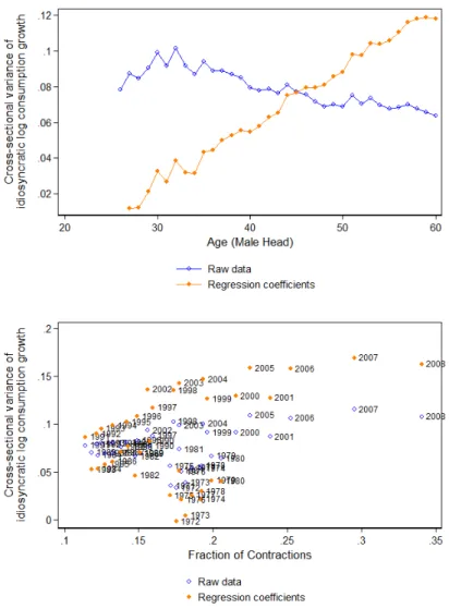
are covered by the sample. In particular, examining equation (10a), shows us that the variances of the persistent shock innovation, 𝜂, accumulate as the cohort ages. Additionally, if the innovation variance is higher in contractionary years, then a cohort that has lived through more contractions will have a higher residual income variance at a given age when compared to cohorts that have lived through fewer contractions. Revisiting the example from the introduction, recall our two groups of 35-year olds. One is born in 1955 and the other is born in 1970. The first enters the workforce at age 25, in 1980. Over the subsequent decade, half of the ten years are classified as a NIPA contraction (see Appendix Table A1 and Figure II). The second enters the workforce at age 25 in 1995. Only two of the following ten years are classified as NIPA contractions. So, the cohort born in 1955 will accumulate more high-variance persistent shocks while aged 25-35. This will show up when comparing the cross-sectional residual variances of cohorts at age 35.30
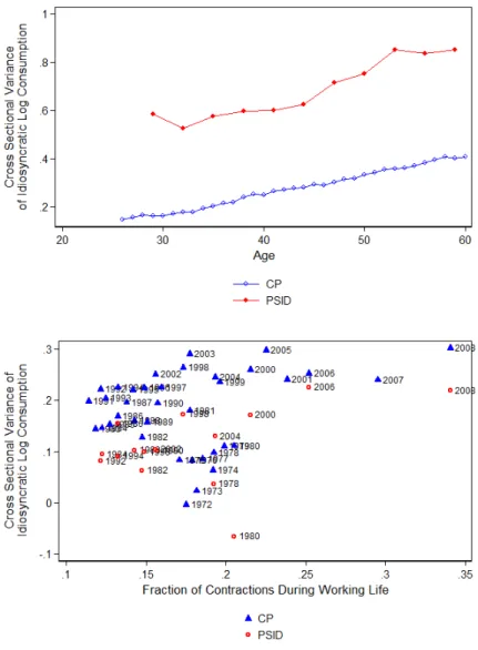
More concretely, consider two cohorts which we observe beginning their working life during the sample period, from 2004-2017. Those born from 1975-1979 enter the workforce between 2000-2004. Those born from 1980-1984 enter the workforce between 2005-2009. In the top panel of Figure III, I plot the residual variance of each of these two cohorts over the number of years that they have been in the workforce (i.e. the x-axis is their age minus 25). One can immediately see that the 1980 cohort has much higher residual variance after only three years in the workforce. This perfectly demonstrates the point that those who have lived through more contractions will show higher variance, as those born from 1980-1985 entered the workforce right before or during the financial crisis. The bottom panel of Figure III shows how the residual variance evolves for all of the cohorts observed in the sample. As we can see, the residual variance always increases as the cohort ages. However, there is dispersion between cohorts at the same age. This is exactly how the parameters in the model are identified via the GMM estimation.
30Recall that this is residual variance, hence I have already controlled for age, family size, region,
The same logic applies to the skewness, as can be seen in equation (10c). If the probability of a large negative income shock is higher (and the probability of a large positive income shocks is lower) during contractions, then skewness during contractionary periods would be more negative. Comparing two cohorts at same age, we should see the cumulative effects of this in a measure of cross-sectional skewness. that is, cohorts that have worked through more contractions will exhibit more negative skewness.
Looking again at (10a), we see that the sum of the variances of the transitory shock and the fixed effect, (𝜇2
𝛼+𝜇2𝜖) is identified as the intercept of the variance profile
over age. The same holds for (𝜇3𝛼 + 𝜇3𝜖). Moreover, the magnitude of the increase in the cross-sectional variance (skewness) over age identifies the variance (skewness) of the persistent shocks. The difference between 𝜇𝑘𝜂,𝐶 and 𝜇𝑘𝜂,𝐸 is identified by the difference of the kth moment of different cohorts of the same age. Roughly speaking, the average of the two represents the rate of increase over the age profile. Additionally, the shape of the profile over age identifies 𝜌; a linear shape implies an autocorrelation coefficient close to one. In summary, variation across age drives the estimates of the autocorrelation coefficient, 𝜌 while variation across time drives the estimates of 𝜇𝑘
𝜂.
Lastly, we can see from equations (10b) and (10d) that the covariance and co-skewness allows me to separately identify 𝜇𝑘
𝛼 and 𝜇𝑘𝜖.
The identification strategy is robust as long as 𝜌 is not close to zero. As 𝜌 approaches zero, it becomes impossible to identify the moments of the AR(1) innova-tion, as the shocks would no longer accumulate. There is ample evidence that there is persistence in these types of shocks, thus I am not concerned that the identification is threatened by a 𝜌 close to zero.31
31See for example, McCurdy (1982) and Abowd and Card (1989) Carroll and Summers (1991),
IV
Results
IV.1
GMM Preview: Graphical Analysis
Many of the main results can be understood by simply looking at the data. From the system that describes the dynamics of 𝑢ℎ𝑖𝑡, (2) and (3), one can see that the estimation of autocorrelation 𝜌 is mostly driven by variation in age. On the other hand, the estimation of the regime switching variance, 𝜇2𝜂,𝐶 and 𝜇2𝜂,𝐸, of the innovation 𝜂ℎ
𝑖𝑡to the persistent shock 𝑧𝑖𝑡ℎ, is driven by variation in time. This motivates a
reduced-form representation of the data. Following Deaton and Paxson (1994), I decompose cross-sectional variances (10a) into cohort and age effects:
˜
𝑉 𝑎𝑟(𝑢ℎ𝑖𝑡) = 𝑎𝑐+ 𝑏ℎ+ 𝑒ℎ,𝑡 (16)
𝑐 = 𝑡 − ℎ is a cohort (birth year) and the parameters 𝑎𝑐 and 𝑏ℎ are cohort and age
effects, respectively.32
I first plot the age coefficients, 𝑏ℎ from the regression in (16) for consumption
in the CP in the top panel of Figure IV in blue. This demonstrates that there is much dispersion when people are young, and that it increases substantially over the lifetime. The residual variance increases from about .15 to .4, or approximately 2.7 times, from age 25 to 60. Moreover, the increase is roughly linear, indicating an autocorrelation coefficient close to one.
The bottom panel of Figure IV plots the cohort coefficients, 𝑎𝑐 but differently.
The x-axis is the fraction of contractions that a cohort has lived through.33 If the variance is indeed counteryclical, then an implication of the model is that a cohort which has worked through more contractions than another at the same age should, on average, exhibit higher cross-sectional variance. Figure IV shows that this indeed
32Regression results are available upon request. 33I.e. Number of contractions at time t
the case. Plotting the cohort coefficients against the fraction of NBER contractions that a cohort has worked through shows an obvious positive relationship. The OLS slope coefficient is .41. In Appendix Figure A2, I show that this positive relationship is robust to each of the three other definitions of contractions.
Next, I turn to the third-moment. I run the same regression as above, but with skewness on the left hand side
˜
𝑆𝑘𝑒𝑤(𝑢ℎ𝑖𝑡) = 𝑎𝑐+ 𝑏ℎ+ 𝑒ℎ,𝑡 (17)
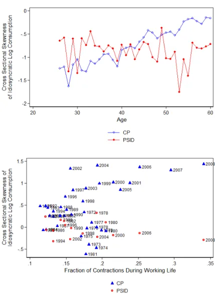
I plot the coefficients in Figure V. From the top panel, we can see that the residual skewness also increases with age. It increases from about -1.5 at age 25-30 to -.2 at age 60. From equation (10b), it’s not obvious that this is what we would expect, as the skewness can take on negative or positive values. If 𝜌 is close to one, then we expect the skenwnesses to accumulate, however many years of varying positive or negative skewness might cancel each other out. What this figure indicates is that, on average, the skewness of the AR(1) innovation is negative, but , on net, it is positive. This makes sense given that the average fraction of NBER contractions in my sample is less than 20 percent, but only if skewness in expansionary years is positive. If we expect the consumption results to match closely those found in income, then the skewness should be more negative during contractions. Hence, with mostly non-contractionary years, the skewness could be more positive and hence accumulate over the lifecycle.
The bottom panel of Figure V shows the cohort coefficients from the regression in (17) against the fraction of NBER contractions that a cohort has worked through. The positive correlation is apparent - The OLS slope coefficient is 5.3. This is a surprising finding. Most of the income literature has found that skewness tends to be procyclical, and thus we might expect skewness to be more negative if a cohort has worked through more contractions. The fact that this is not the case indicates that consumption may not exhibit the same pro-cyclical skewness that income does. In Appendix Figure A3, I show that this positive relationship is robust to each of the
three other definitions of contractions. I’ll return to this discussion in Section 4.2, when I discuss the GMM estimation results, which verify this conjecture.
Turning now to the PSID data, the same figures show consumption data in the PSID in red. Looking again at the top panel of Figure IV, we see that the cross-sectional variance also increases in age, going from about .5 at age 30 to .8 at at 60, or about 1.6 times.34 This is smaller than the increase observed in the CP data, but the shape of the increase is also close to linear, indicating unity in the autocorrelation coefficient. Note that the variances are also higher on average in the PSID, which makes sense given that the PSID consumption covers many more products. The bottom panel of Figure IV shows the cohort coefficients against the fraction of contractions the cohort has worked though. Again, we observe a positive relationship, with an OLS coefficient of .48.
The top panel of Figure V shows how the cross-sectional skewness evolves with age. Unlike with the CP data, it is relatively flat. This indicates that the persistent shocks to consumption are not, on net, positive in this data. Rather, they must be negative on average, with some positive and negative realizations canceling each other out as an individual accumulates shocks over the lifecycle. The bottom panel shows a negative relationship between the cross-sectional skewness and the fraction of contractions worked: the OLS coefficient is -.88. This contrasts the very large positive coefficient that is found when looking at consumption in the CP, but indicates that consumption, as measured by the PSID, may exhibit similar procyclical skewness as does income. However, the standard error on the OLS coefficient is .67, indicating that is it very imprecisely estimated and not significantly different from zero. I will revisit this discussion following the estimation results in the next section.
IV.2
Estimation Results
The estimation begins with the first stage regression specified in equation (1) and repeated here for clarity:
𝑐ℎ𝑖,𝑡 = 𝜃0+ 𝜃1𝑇𝐷(𝑌𝑡) + 𝜃𝑇2𝑥 ℎ 𝑖,𝑡+ 𝑢
ℎ
𝑖𝑡 (18)
Recall that the year dummies 𝐷(𝑌𝑡) are used to capture the aggregate component of
consumption and the vector 𝑥ℎ
𝑖𝑡captures the deterministic component of consumption.
𝑥ℎ𝑖𝑡 contains a cubic in age for the head of household, family size, education level of the head of household, race dummies, state dummies, and an inequality control in the form of the initial residual variance of food consumption for the year in which the head of household enters the workforce. Table VII shows the results of this regression. The estimates are quite similar to previous studies, including STY and others, such as Hubbard, Skinner, and Zeldes (2004). Consumption is concave in age and increasing in family size. Also note that the coefficient on the initial standard deviation of food consumption is large and highly significant. This confirms evidence that inequality has increased over time, hence this initial dispersion affects the level of consumption later in life.35
A few differences from the regression in STY are worth noting. First, the educa-tion coefficient is negative. It is also economically small and barely significant, with a t-statistic of less than two. In STY, the coefficient is positive and highly significant, indicating a strong positive relationship between education and earnings. Another important difference is the R-squared values. In the regression presented here, these variables explain 12.8 percent of the variation in log of consumption. In STY, the R-squared is 23 percent. Additionally, STY do not include race or region dummies, hence they have fewer explanatory variables but more explanatory power. This is
35In Appendix Table A3, I show this regression without the inequality control. Note that the
coefficients on other observables do not substantially change, nor does the R-squared. This validates the use of this proxy for inequality as a control, as without it, its impact would be captured by the residual, which is exactly what I want to avoid.
relevant, as the object that I am primarily interested in is the residual of this regres-sion. A lower R-squared indicates that there may be more unobserved factors that influence residual consumption than income.
Running the regression in (18) allows me to identify the residual, 𝑢ℎ𝑖𝑡which follows the process in equation (2). I estimate the parameters specified via the systems in (10) and (15) using GMM. The results are shown in Table IX. The first three columns shows the results for the CP data for three of the contraction definitions.36 Looking
first at the results for the autocorrelation coefficient, 𝜌, we see that it is indeed close to unity and quite precisely estimated.37 On average, the sum of the variances of the
fixed effect and the transitory shock, shown in the 2nd and 3rd row respectively, is .1587. This matches well with the intercept in the top panel of Figure IV, which is approximately .13.
Now turning to the results for the second moment of the AR(1) innovation, the countercyclical volatility is immediately apparent. The standard deviation rises by an average of 23 percent from expansion to contraction.38
The last four rows in Table IX show the results for the parameters of the third moment. Again, the sum of the skewness of the transitory shock and the fixed effect identifies the intercept in the top panel of Figure V. The average sum of the two is -1.56, compared to the intercept of -1.54 in the figure. Additionally, the fact that the skewness of the transitory shock, 𝜇3𝜖 is highly negative confirms that transitory shocks to consumption are negatively skewed: negative shock realizations have more weight than positive ones.
Moving now to the skewness of the AR(1) innovation, we see that 𝜇3𝜂,𝐶 and 𝜇3𝜂,𝐸
36I exclude the results for the unemployment contractions as they are almost identical to those
of the NBER indicators. The NBER and unemployment indicators are highly correlated (see Table VI).
37The 95 percent confidence interval for the estimate using the NBER indicators is [.9764, .9988]. 38The differences between 𝜇2
𝜂,𝐶 and 𝜇 2
𝜂,𝐸 are significantly different at the 1 percent level for the
NIPA and Negative returns definition; they are significantly different at the 10% level for the NBER definition.
are not significantly different from each other. Additionally, they are very imprecisely estimated with large confidence bands. Although the estimation results with each measure of contractions do indicate that there is slightly procyclical skewness (i.e. 𝜇3
𝜂,𝐶 is more negative that 𝜇3𝜂,𝐸 in all cases), there is not enough power to reject that
the two estimates are equal.
Next, I discuss the complementary estimation results using the PSID data. The sample sizes are much smaller in this data, with between 3,000-6,000 observations per year (see Table III). Additionally, the survey is only biannual from 1999-2017, thus I have only 10 years of observations, as opposed to the 14 in the CP data. Even so, the results, shown in the last three columns of Table IX, are comparable. The autocorrelation coefficient is close to one for each of the three recession definitions. The volatility exhibits even more countercyclicality here than in the CP, rising by 68, 30, and 66 percent for each of three recession types, respectively.39 Moreover, the
skewness still does not change substantially between the two states, and is imprecisely estimated.
IV.3
Comparison to Income Results
In order to compare the dynamics of consumption to those of income, I first repeat the analysis on the PSID over the same sample period, 1999-2017. Beginning again with the graphical analysis, the top panel of Figure VI shows the age coefficients from the regression in (16) with the variance of residual income on the y-axis. As with consumption, the variance increases with age, rising by about 1.5 times from age 25 to 60. The magnitude of the increase is similar to that found in PSID consumption. The initial dispersion, or the sum of the variance of the fixed effect and the transitory shock, is higher in the income data, about .55 versus .38. The bottom panel of Figure VI plots the cohort coefficients from the regression in (16) against the fraction of
39For each of the recession types, the conditional variances for expansions and contractions are
contractions that a cohort has worked through. As with consumption, the relationship is positive, with an OLS slope coefficient of .57, which is slightly higher than the coefficient for consumption (.48). Hence, it seems that income and consumption in the PSID both exhibit strong autocorrelation and countercyclicality.
Looking now at Figure VII, we see that the dynamics of the third moments of income in the PSID are similar to those of consumption in the PSID as well. As with consumption, the top panel shows that the cross-sectional skewness is not increasing over the lifecycle, but rather stays relatively flat and negative. This indicates that the persistent shock to income is not positive, on net, as it was with consumption. In the PSID, negatively skewed shocks dominate as the innovations accumulate. Looking at the bottom panel, we see that the OLS slope coefficient is -.11, with a very large standard deviation of 1.15.40, compared to an imprecisely estimated measure of -.87 in the PSID consumption data. Although this slope is small in magnitude and not significantly different from zero, it provides some weak evidence of possible procycli-cality of skewness in the PSID income data. It’s important to interpret these results with caution, though, due to the small sample size in the PSID and imprecision of measurement with higher order moments.
In Table X, I show the estimation results on PSID income from 1999-2017. As with consumption, the autocorrelation coefficient, 𝜌, is close to unity. The condi-tional standard deviation, 𝜇2
𝜂 rises by approximately 34 percent from expansion to
contraction. This is very similar to increase for consumption, which was 30 percent for the full sample in the PSID using NBER indicators. The difference between the state-conditional variances for income is significantly different at the 95 percent level. In the skewness here, however, we see that it does substantially increase in magni-tude from expansion to contraction. The values are significantly different from each other at the 95th percent.41 Hence, there is evidence that the skewness of income is
40When using the definitions for contractions that rely on the equity premium and GDP growth,
the OLS coefficients are -1.12 with a standard deviation of .97 and -.66 with a standard deviation of .65, respectively.
procyclical; this evidence is absent in the consumption data.
In Table X, I also duplicate the main estimation results using NBER indicators from STY Table 2, for comparison. Besides the fact that STY used data on income while I am using data on consumption, their estimation was also for the time period from 1968-1993, while mine is from 2004-2017 in the CP and 1999-2017 in the PSID. Hence, there may be differences due to the time period, rather than due to differences in income and consumption. Comparing these results to my results for income, a few differences are immediately apparent. First, the variance of the fixed effect and the transitory shock are higher in the more recent data. Similarly, the conditional variances of the persistent shock are larger. On the other hand, the increase from expansion to contraction is much smaller in the updated data. In my estimation from 1999-2017, it rises by about 33 percent from peak to trough, versus 69 percent in the STY estimation.
To summarize, residual income and consumption both exhibit strong autocorre-lation and countercyclicality in the variance of the persistent shock using data from the PSID from 1999-2017. This is also observed by STY using income data from the PSID from 1968-1993. However, the magnitude of the increase of the variance from peak to trough in STY is much larger than I find in the more recent data for both consumption and income. Moreover, I do observe procyclical skewness in the PSID income data, with the skewness being almost seven times more negative during contractions. However, I do not observe a similar pattern in the consumption data; the conditional skewness in each state are not statistically different from each other.
IV.4
Stockholders
One of the primary issues with consumption-based asset pricing is limited par-ticipation. Namely, when not all consumers participate in the stock market, the SDF
is attenuated and therefore the equity premium is overestimated.42 For this reason, it is difficult to make asset pricing implications when looking at the consumption of individuals who may not participate in the stock market.
To deal with this, I re-estimate the parameters on specific subsamples of the population that are most likely to own stocks. The CP does not contain data on stock ownership, however there are several proxies available in the demographic information that is provided. First, I drop those who have less than a college education, leaving about 40 percent of the sample. Second, I drop those who have an income of fewer than 100,000 dollars, leaving about 20 percent of the sample. Lastly, I fit a model based on the PSID data, which does include stock ownership information, to predict stock ownership in the CP. Following Malloy, Moskowitz and and Vissing-Jorgenson (2009), I fit a probit model of stock ownership on age, income, education, and year effects. I then apply these estimates to the CP data to predict stock ownership. Appendix Table A7 shows the results of the probit regression. Table IV shows the estimated stock ownership in the CP data. Following this method, approximately 16 percent of the estimation sample in the CP is predicted to own stocks.43
The results for the estimation on the high-education, high-income, and stock owning subsamples are shown in Table XI. This table uses the NBER recession in-dicators, and thus is comparable with the first column of Table IX. The results are qualitatively similar across each of the subsamples and the full sample. However, there are some notable differences. First of all, these subsamples exhibit slightly more countercyclicality in the estimates of the conditional variance of the persis-tent shock, particularly the high income and stock holding samples. The standard deviation rises by 28 percent, 33 percent and 34 percent from economic expansion to contraction for each subsample, respectively, compared to 23 percent for the full sample. Second, the variances of the transitory shock and the fixed effect (the sum of which identifies the initial dispersion), are lower for the high education and
stock-42See Campbell (2018) and Brav, Constantinides and Geczy (2002) for a more thorough discussion. 43Summary statistics for each of these subpanels are shown in Appendix Tables A8-A10,