HAL Id: tel-01712290
https://tel.archives-ouvertes.fr/tel-01712290
Submitted on 19 Feb 2018
HAL is a multi-disciplinary open access
archive for the deposit and dissemination of sci-entific research documents, whether they are pub-lished or not. The documents may come from teaching and research institutions in France or abroad, or from public or private research centers.
L’archive ouverte pluridisciplinaire HAL, est destinée au dépôt et à la diffusion de documents scientifiques de niveau recherche, publiés ou non, émanant des établissements d’enseignement et de recherche français ou étrangers, des laboratoires publics ou privés.
statistical signal processing
Gia-Thuy Pham
To cite this version:
Gia-Thuy Pham. Applications of large randommatrix to high dimensional statistical signal processing. Statistics [math.ST]. Université Paris Est Marne la Vallée, 2017. English. �tel-01712290�
THÈSE
pour obtenir le grade de docteur délivré par
Université Paris-Est
Spécialité: Traitement du signal
présentée et soutenue publiquement par
Gia-Thuy P
HAMle 28 Février 2017
Applications des grandes matrices aléatoires au traitement du
signal de grandes dimensions
Applications of large random matrix to high dimensional statistical signal processing
Directeur de thèse : Philippe LOUBATON
Composition de la commission d’examen
Xavier MESTRE, Professeur Rapporteur
Jianfeng YAO, Professeur Rapporteur
Frédéric PASCAL, Professeur Examinateur
Walid HACHEM, Professeur Examinateur
Remerciements 2
1 Introduction 6
1.1 Introduction . . . 6
1.2 Review of useful known results. . . 7
1.3 Behaviour of the eigenvalues of the empirical spatio-temporal covariance matrices of tem-porally and spatially complex Gaussian noise. . . 15
1.4 Contributions of the thesis. . . 16
2 Spatial-temporal Gaussian information plus noise spiked model 21 2.1 Introduction . . . 21
2.2 Behaviour of the largest eigenvalues and corresponding eigenvectors ofΣ(L)N Σ(L)∗N . . . 22
2.3 Detection of a wideband signal. . . 27
2.4 Estimation of regularized spatio-temporal Wiener filters . . . 35
2.5 Performance analysis of spatial smoothing schemes in the context of large arrays . . . 43
3 Complex Gaussian information plus noise models: the deterministic equivalents 58 3.1 Notations and useful tools. . . 58
3.2 Random variables notations and tools. . . 65
3.3 Overview of the results of Chapter. . . 66
3.4 Poincaré-Nash variance evaluations . . . 67
3.5 Expression of matricesE(Q) and E( ˜Q) obtained using the integration by parts formula . . . 71
3.6 Preliminary controls of the error termsΥ, ˜Υ . . . 82
3.7 The deterministic equivalents: existence and uniqueness . . . 87
3.8 Convergence towards the deterministic equivalents: the normalized traces . . . 90
3.9 Convergence towards the deterministic equivalents: the bilinear forms . . . 93
3.A Proof of lemma 3.5.1 . . . 95
4 Convergence towards spiked model : the case of wideband array processing models 96 4.1 Introduction . . . 96
4.2 Overview of the results. . . 97
4.3 Simplified behaviour of the bilinear forms of QN(z) and ˜QN(z). . . . 98
4.4 Application to regularized estimated spatial-temporal Wiener filters in large system case . 108 4.5 Asymptotic behaviour of the SINR . . . 109
4.A Proof of lemma 4.3.1 . . . 118
Mes premiers remerciements iront sans doute à Philippe Loubaton. Il m’a inspiré de sa patience, sa compréhension et sa persévérance. Son expertise et ses connaissances sont splendides, cela aide à ré-soudre des problèmes plus rapidement. Perturbé par les tâches administratives du LabEx, du CNRS, et les enseignements, Philippe a toujours su se montrer disponible, de bonne humeur, d’efficacité. En particulier, pour moi, Philippe est comme le deuxième père, qui m’écoute et qui me donne des conseils. Phillipe, tu es un exemple que je vais continuer à suivre pendant toute ma carrière !
I also want to thank Xavier Mestre and Jian-Feng Yao for accepting to be rapporteurs of this thesis, and I thank them for their positive comments. I have met Xavier in many occasions, especially during SSP 2016 in Palma de Mallorca with a very nice dinner. In addition, inspired by Xavier’s idea in his paper, back in 2006, that we could have a publication. My gratitude also goes to Walid Hachem,Frédéric Pascal and Inbar Fijalkow for accepting to participate to the jury of my thesis.
Ce fut un plaisir de travailler avec Pascal Vallet. C’était le début de ma thèse, Pascal n’a pas hésité de me donner un cours, transmettant ses connaissances de manière très enthousiaste. Ses idées sont enfin matérialisées par notre publication sur TSP. J’espère sincèrement pouvoir continuer à travailler avec lui dans l’avenir.
Durant ces trois années, j’ai travaillé au sein de l’équipe signal du laboratoire IGM de Marne-la-Vallée. Je remercie tous les collègues pour la bonne ambiance qu’ils ont su apporter chaque jour: Sonja et Mohamed Ali, mes colocataires de bureau 4B048, qui ont dû me supporter durant ces années, les thésards Feriel, Yosra, Aurélie, Audrey, Mai-Quyen, Mireille, Safa, Zakaria..., à Jamal et Abdellatif pour les discussions enrichissantes, sans oublier Samuele pour les parties échecs, Carlos, Siqi, Daniel, Alain,... pour les matchs de foot, et aussi Emilie et Jean-Christophe pour leurs conseils. Corinne Palescandolo et Patrice Herault méritent amplement des remerciements, pour leur aide et leurs grandes compétences dans les domaines administratif et informatique, respectivement.
Mes derniers remerciements seront consacrés à mes proches. Je remercie mes parents pour leur soutien et toute leur aide, surtout pour leur confiance continue en leur fils qui se trouve à l’autre bout du monde, à 12000 km d’eux. Je remercie ma mère pour son esprit fort, qui m’a appris à ne jamais abandonner dans la vie. Je remercie mon père pour son éducation, ses cours de maths, d’échecs, de foot,etc, malgré qu’il soit hospitalisé depuis quelques temps, mais il garde toujours un bon esprit et de l’optimisme. Je remercie également ma petite soeur d’avoir partagé notre enfance, et qui me motive à devenir un bon exemplaire du grand frère. Je remercie également tous mes amis, pour leur encourage-ment et pour avoir pris régulièreencourage-ment des nouvelles. Finaleencourage-ment, mes remercieencourage-ments vont à Thai-Hoa, celle qui a partagé ses 7 ans de jeunesse avec moi, qui restait à côté de moi et qui m’a soutenu durant tous ces années. Surtout, je la remercie d’avoir découvert mon anomalie cardiaque, qui a sauvé ma vie. Malgré que l’on ait pris des chemins différents, j’espère que l’on se croisera un jour.
Cette thèse porte sur des problèmes de statistiques mettant en jeu une série temporelle multivariable yn de grande dimension M définie comme la somme d’un bruit gaussien blanc temporellement et spatiale-ment et d’un signal utile généré comme la sortie d’un filtre 1 entrée / M sorties à réponse impulsionnelle finie excité par une séquence déterministe scalaire non observable. Si l’on suppose que y est observé entre les instants 1 et N, un bon nombre de techniques existantes sont basées sur des fonctionnelles de la matrice de covariance empirique ˆRLdes vecteurs de dimensions ML (y(L)n )n=1,...,Nobtenus en em-pilant les vecteurs yk entre les instants n et n + L − 1, où L est un paramètre bien choisi. Lorsque l’on est en mesure de collecter un nombre d’observations très nettement plus grand que la dimension ML des vecteurs (y(L)n )n=1,...,N, ˆRL a le même comportement en norme spectrale que son espérance
math-ématique, et cela permet d’étudier les techniques d’inférences basés sur ˆRL par le biais de techniques
classiques de statistique asymptotique. Dans cette thèse, nous nous intéressons au cas où ML et N sont du même ordre de grandeur, ce que nous modélisons par des régimes asymptotiques dans lesquels M et N tendent tous les deux vers l’infini, et où le rapport ML/N converge vers une constante non nulle, L pou-vant aussi croître avec M et N. Les problèmes que nous résolvons dans ce travail nécessitent d’étudier le comportement des éléments propres de la grande matrice aléatoire ˆRL. Compte tenu de la structure
particulière des vecteurs (y(L)n )n=1,...,N, ˆRL coïncide avec la matrice de Gram d’une matrice Hankel par
blocΣL, et cette spécificité nécessite le développement de techniques appropriées.
Dans le chapitre 2, nous nous intéressons au cas où le nombre de coefficients P de la réponse im-pulsionnelle générant le signal utile et le paramètre L restent fixes quand M et N grandissent. La ma-triceΣL est alors une perturbation de rang fini de la matrice Hankel par bloc WL constituée à partir
du bruit additif. Nous montrons que les éléments propres de ˆRL se comportent comme si la matrice
WLétait à éléments indépendants et identiquement distribués. Cela nous permet d’aborder l’étude de
tests de détection du signal utile portant sur les plus grandes valeurs propres de ˆRLainsi que la mise en
évidence de nouvelles stratégies de détermination du paramètre de régularisation de filtres de Wiener spatio-temporels estimés à partir d’une séquence d’apprentissage. Techniquement, ce dernier point est abordé en caractérisant le comportement asymptotique des éléments de la résolvente de la matrice ˆRL.
Nous montrons enfin également que ces résultats permettent d’analyser le comportement d’algorithmes sous-espace de localisation de sources bande étroite utilisant la technique du lissage spatial.
Dans le chapitre 3, motivés par le cas où P et L peuvent tendre vers l’infini, nous nous écartons quelque peu du modèle initial, et supposons que la matriceΣLest la somme de la matrice aléatoire
Han-kel par bloc WLavec une matrice déterministe sans structure particulière. En utilisant des approaches
basées sur la transformée de Stieltjes et des outils adaptés au caractère gaussien du bruit, nous montrons que la distribution empirique des valeurs propres de ˆRLa un comportement déterministe que nous
car-actérisons. Sous réserve L2/MN tende vers 0, nous faisons de même pour les éléments de la résolvante de ˆRL.
Dans le chapitre 4, nous revenons au modèle initial, mais supposons que P et L tendent vers l’infini au même rythme. Dans ce contexte, la contribution du signal utile à la matriceΣLest une matrice dont le
les résultats du chapitre 3, nous établissons que si L2/MN tende vers 0, les éléments de la résolvante de ˆRL se comportent comme les éléments d’une matrice déterministe qui coïncide avec l’équivalent
déterministe de la resolvente d’un modèle information plus bruit dans lequel les éléments de la matrice de bruit sont indépendants et identiquement distribués. Dans le cas où L/M tend vers 0, ceci nous permet d’étendre les résultats du chapitre 2 relatifs à la détermination du paramètre de régularisation des filtres de Wiener spatio-temporels estimés à partir d’une séquence d’apprentissage.
This thesis focuses on statistical problems involving a multivariate time series yn of large dimension M defined as the sum of gaussian white noise temporally and spatially and a useful signal defined as the output of an unknown finite impulse response single input multiple outputs system driven by a deterministic scalar nonobservable sequence. Supposing (yn)n=1,...,N is available, a number of exist-ing methods are based on the functionals of empirical covariance matrix ˆRLof ML–dimensional vectors
(y(L)n )n=1,...,Nobtained by stacking the vectors (yk)k=n,...,n+L−1, where L is a relevant parameter. In the case where the number of observations N is much larger than ML the dimension of vectors (y(L)n )n=1,...,N, ˆRL
behaves as its mathematical expectation in the sense of spectral norm. This allows us to study the infer-ence technique based on ˆRLvia classical techniques of asymptotic statistics. In this thesis, we interested
in the case where ML and N have the same order of magnitude, we call this the asymptotic regimes in which M and N converge towards infinity, such that the ratio MLN converges towards a strictly positive constant, given that L may scale with M, N. To solve the problems in this work, it is necessary to investi-gate the behaviour of the eigenvalues and eigenvectors of the random matrix ˆRL. Taking account of the
particular structure of vectors (y(L)n )n=1,...,N, ˆRLcoincides with the Gram matrix of a block-Hankel matrix
ΣL, and this specificity requires the development of appropriate techniques.
In chapter 2, we interested to the case where the number of coefficients P of the finite impulse re-sponse generated the useful signal and the parameter L remain fixed when M, N grow large. As a con-sequence, the matrixΣLis a finite rank perturbation of block-Hankel matrix WL composed of additive
noise. We prove that eigenvalues and eigenvectors of ˆRLbehave as if the entries of matrix WL are
inde-pendent and identically distributed. This allows us to construct detection tests of useful signal based on largest eigenvalues of ˆRLand to develop new estimation strategies of the regularization parameter of the
spatio-temporal Wiener filter estimated from a training sequence. This approach is characterized by the asymptotic behaviour of the resolvent of matrix ˆRL. We also prove that these results provide consistent
subspace estimation methods for source localization using spatial-smoothing scheme.
In chapter 3, motivated by the case where P and L may converge towards infinity, we move off some-what the initial model. We suppose that the matrixΣLis the sum of the block-Hankel random matrix WL
with a deterministic matrix without particular structure. Using the approaches based on Stieltjes trans-form and tools adapted to gaussian noise, we prove that the empirical eigenvalue distribution of ˆRLhas
deterministic behaviour which we shall describe. Provided MNL2 converges towards 0, we do likewise for the elements of the resolvent of ˆRL.
In chapter 4, we return to the initial model, but we suppose that P, L converge towards infinity with the same rate. In this context, matrixΣLis a matrix whose rank goes to infinity, and thus the techniques
employed in chapter 2 are not applicable. Using the results obtained in chapter 3, we establish that whenMNL2 goes to 0, the elements of the resolvent of ˆRLbehave as the elements of a deterministic matrix
which coincides with the deterministic equivalent of the resolvent of the information plus noise model in which entries of the noise matrix are independent and identically distributed. In the case where ML goes to 0, this allows us to extend the results of chapter 2 related to the determination of the regularization parameter of the spatial-temporal Wiener filter estimated from a training sequence.
Introduction
1.1 Introduction
Due to the spectacular evolution of data acquisition devices and sensor networks, it becomes common to be faced to multivariate signals of high dimension. Very often, the sample size that can be used in practice to perform statistical inference cannot be much larger than the dimension of the observation because the duration of the signals are limited, or because their statistics are not time-invariant over large enough temporal windows. In this context, it is well established that fundamental statistical signal processing techniques implemented in existing systems (e.g., source detection, source localisation, esti-mation of various kinds of spatial and spatio-temporal filters, or of equalizers, blind source separation, blind deconvolution and equalization,...) show poor performance. It is therefore of crucial importance to revisit the corresponding problems, and to be able to propose new algorithms with enhanced per-formance. In the last decade, a number of mathematical tools were thus developed in the context of high-dimensional statistical signal processing. Among others, we mention the use of possible sparsity of certain parameters of interest, and large random matrices. This thesis concentrates on the development of large random matrix tools, and to their applications to important high-dimensional statistical signal processing problems.
Large random matrices have been proved to be of fundamental importance in mathematics (high di-mensional probability and statistics, operator algebras, combinatorics, number theory,...) and in physics (nuclear physics, quantum fields theory, quantum chaos,..) for a long time. The introduction of large ran-dom matrix theory in electrical engineering is more recent. It was introduced at the end of the nineties in the context of digital communications in order to analyse the performance of large CDMA and MIMO systems. Except the pioneering work of Girko ([26], [27]), the first works using large random matrix the-ory in the context of multivariate statistical signal processing were published in the second part of the 2000s, see e.g. [53], [54], [55], [40], [57], [43], [58]. These works were followed by a number of subse-quent contributions, e.g. [12], [16], [17], [18], [19], [72], [33], [74], [79], [80]. The common point of the above mentioned works is to address statistical inference problems for the narrow band array processing model, also called the linear static factor model in the statistical terminology. In this context, the obser-vation is a M-dimensional signal yn defined as a noisy version of a low rank K useful signal on which various informations have to be retrieved from samples (yn)n=1,...,N. In particular, one may want to de-tect the presence or the absence of the useful signal, to estimate its rank K, the corresponding signal subspace, or to estimate certain parameters (e.g. direction of arrival). A number of statistical inference methods are based on the observation that the relevant informations are contained in the "true" spatial covariance matrix R = E(yny∗n), and that, in the case where M << N, the empirical spatial covariance ma-trix ˆR behaves as R. Therefore, many detection / estimation schemes use functionals of ˆR, which, when
M << N, behave as the corresponding functionals of R. When M and N are large and of the same order of magnitude, it is well established that ˆR is a poor estimate of R in the sense that functionals of ˆR do
not behave as the functionals of R. The above mentioned papers developed methodologies that allow to evaluate the behaviour of functionals of ˆR in the asymptotic regime M and N converge towards
infin-ity at the same rate, and to take benefit of the corresponding results to propose improved performance statistical inference schemes.
In the present thesis, we address statistical inference problems for the wide band array processing model in which the useful signal is low rank in the frequency domain, or, in other words, coincides with the output of an unknown K inputs / M outputs filter (with K < M) driven by a K–dimensional time series. In this case, the empirical spatial covariance matrix does not convey enough information on the low rank component, and several inference schemes are rather based on empirical spatio-temporal covariance matrices ˆR(L) defined as the empirical covariance matrices of augmented ML–dimensional vectors y(L)n = (yTn, . . . , yTn+L−1)Twhere L is a relevant parameter. Our goal is thus to study the asymptotic behaviour of functionals of random matrices ˆR(L) when M and N converge towards infinity, to use the corresponding results to analyze the performance of traditional detection / estimation schemes, and to propose improved methods. The main originality of this research program follows from the particular structure of the ML×N augmented observation matrix YL= (y(L)1 , . . . , y(L)N ). This matrix has a block-Hankel
structure, so that the analysis of the asymptotic behaviour of ˆR(L)= YLY∗L/N needs the establishment of
new results.
1.2 Review of useful known results.
In this section, we review some fundamental results concerning large empirical covariance matrices.
1.2.1 The Marcenko-Pastur distribution.
The Marcenko-Pastur distribution was introduced 40 years ago in [52], and plays a key role in a num-ber of high-dimensional statistical signal processing problems. In this section, (vn)n=1,...,Ndenotes a se-quence of i.i.d. zero mean complex Gaussian random M–dimensional vectors for whichE(vnv∗n) = σ2IM.
We consider the empirical covariance matrix 1 N N X n=1 vnv∗n
which can also be written as
1 N N X n=1 vnv∗n= WNW∗N
where matrix WNis defined by WN=p1N(v1, . . . , vN). WNis thus a complex Gaussian matrix with
inde-pendent identically distributedNc(0,σ
2
N) entries. When N → +∞ while M remains fixed, matrix WNW∗N
converges towardsσ2IMin the spectral norm sense. In the high-dimensional asymptotic regime defined
by
M → +∞,N → +∞,dN=
M
N→ d > 0 (1.2.1)
it is well understood that kWNW∗N− σ2IMk does not converge towards 0. In particular, the empirical
distribution ˆµN=M1 PMm=1δˆλm,Nof the eigenvalues ˆλ1,N≥ . . . ≥ ˆλM,Nof WNW∗Ndoes not converge towards
of parameters (d ,σ2) defined as probability measure dµd ,σ2(λ) = δ0[1 − d−1]++
p
(λ − λ−) (λ+− λ)
2σ2dπλ 1[λ−,λ+](λ)dλ
withλ−= σ2(1 −pd )2andλ+= σ2(1 +pd )2. Then, the following result holds.
Theorem 1.2.1. The empirical eigenvalue value distribution ˆµNconverges weakly almost surely towards
µd ,σ2 when both M and N converge towards +∞ in such a way that dN= M
N converges towards d > 0.
Moreover, it holds that
ˆλ1,N → σ2(1 + p d )2a.s. (1.2.2) ˆλmin(M,N) → σ2(1 − p d )2a.s. (1.2.3)
We also observe that Theorem 1.2.1 remains valid if WNis a non necessarily Gaussian matrix whose
i.i.d. elements have a finite fourth order moment (see e.g. [5]). Theorem 1.2.1 means that when ratio MN is not small enough, the eigenvalues of the empirical spatial covariance matrix of a temporally and spa-tially white noise tend to spread out around the variance of the noise, and that almost surely, for N large enough, all the eigenvalues are located in a neighbourhood of interval [λ−,λ+]. While the spreading of the eigenvalues is not an astonishing phenomenon, it is remarkable that the behaviour of the eigenvalues can be characterized very precisely.
In order to establish the convergence of ˆµNtowardsµd ,σ2, the simplest approach consists in studying
the asymptotic behaviour of the Stieltjes transform ˆmN(z) of ˆµNdefined as
ˆ mN(z) = Z R+ 1 λ − zd ˆµN(z) = 1 M M X m=1 1 ˆλm,N− z (1.2.4) and to establish that for each z ∈ C − R+, it holds that
lim
N→+∞mˆN(z) = md ,σ
2(z) a.s., (1.2.5)
where md ,σ2(z) =RR+λ−z1 dµd ,σ2(λ) represents the Stieltjes transform of µd ,σ2. Function md ,σ2 is known
to be the unique Stieltjes transform of a probability measure carried byR+satisfying the equation md ,σ2(z) =
1 −z +1+σ2d mσ2
d ,σ2(z)
(1.2.6)
for each z. md ,σ2(z) can also be defined as the first component of the solution of the coupled equation
md ,σ2(z) = 1 −z¡1 + σ2m˜d ,σ2(z)¢ (1.2.7) ˜ md ,σ2(z) = 1 −z¡1 + σ2d md ,σ2(z)¢
The second component ˜md ,σ2(z) of the solution of (1.2.7) then coincides with −(1 − d)/z + d md ,σ2(z) i.e.
with the Stieltjes transform of (1 − d)δ0+ d µd ,σ2. It is easily seen that
(1 − d)δ0+ d µd ,σ2= µd−1,σ2d (1.2.8)
Therefore, it also holds that
˜
for each z ∈ C−R+. In order to establish (1.2.5), it is sufficient to use a Gaussian concentration argument, and to prove thatE( ˆmN(z)) satisfies a perturbed version of (1.2.6). In the Gaussian case, this last point
can be addressed using the integration by parts formula and the Poincaré-Nash inequality, see below for more details. We also mention that function wd ,σ2(z) defined by
wd ,σ2(z) =
1
zmd ,σ2(z) ˜md ,σ2(z)
(1.2.10) is analytic onC − [λ−,λ+], verifies Im(w (z))Im(z) > 0 if z ∈ C − R, wd ,σ2(λ−) = −σ2
p
d and wd ,σ2(λ+) = σ2
p d . Moreover, wd ,σ2(λ) increases from −∞ to −σ2
p
d whenλ increases from −∞ to λ−, wd ,σ2(λ) increases
fromσ2pd to +∞ when λ increases from λ+to +∞, and the set {wd ,σ2(λ),λ ∈ [λ−,λ+]} coincides with
the half circle {σ2pd eiθ} whereθ increases from −π to 0. Using (1.2.7), it is possible to express md ,σ2(z)
in terms of wd ,σ2(z). More precisely,z ˜m 1
d ,σ2(z)= −(1 + σ 2d m d ,σ2(z)) so that wd ,σ2(z) = − 1 + σ2d md ,σ2(z) md ,σ2(z) Solving w.r.t. md ,σ2(z) leads to md ,σ2(z) = − 1 wd ,σ2(z) + σ2d (1.2.11) It can be shown similarly that
˜
md ,σ2(z) = −
1 wd ,σ2(z) + σ2
(1.2.12) Plugging (1.2.11) into (1.2.6), we obtain that wd ,σ2(z) is solution of the equation
φd ,σ2¡wd ,σ2(z)¢ = z (1.2.13)
for each z ∈ C where φd ,σ2(w ) is the function defined by
φd ,σ2(w ) =(w + σ
2)(w + σ2d )
w (1.2.14)
It is useful to notice that if QW,N(z) denotes the resolvent of matrix WNW∗Ndefined by
QW,N(z) =¡WNW∗N− zIM¢−1 (1.2.15)
then ˆmN(z) coincides with M1Tr¡QW,N(z)¢. We also note that it is possible to establish a stronger result,
i.e. for each z ∈ C − R+,
a∗N¡QW,N(z) − md ,σ2(z)IM¢ bN→ 0 a.s. (1.2.16)
for each deterministic vectors aN, bNfor which supN(kaNk, bNk) < +∞. A similar result holds for ˜QW,N(z)
defined as the resolvent of W∗NWN, i.e.
˜
QW,N(z) =¡W∗NWN− zIN
¢−1
(1.2.17) More precisely, it holds that
˜a∗N¡˜
QW,N(z) − ˜md ,σ2(z)IN¢b˜N→ 0 a.s. (1.2.18)
for each deterministic vectors ˜aN, ˜bNfor which supN(k˜aNk, ˜bNk) < +∞. Moreover, for each z ∈ C − R+, it
holds that
a∗N¡QW,N(z)WN
¢˜
bN→ 0 a.s. (1.2.19)
Finally, convergence properties (1.2.16, 1.2.18, 1.2.19) hold uniformly w.r.t. z on each compact subset of C∗− [λ−,λ+].
1.2.2 The Information plus noise spiked models.
An information plus noise model is a M × N random matrix model ΣNdefined as
ΣN= BN+ WN (1.2.20)
where complex Gaussian random matrix WNis defined as above, and where BNis a deterministic M × N
matrix. In the asymptotic regime (1.2.1), this kind of models were initially studied by Girko (see e.g. [26]) , later by Dozier-Silverstein (see [20], [21]), and by [32] in the case where the entries of WN are
independent but not necessarily identically distributed. We denote by (ˆλm,N)m=1,...,Mthe eigenvalues of
ΣNΣ∗Narranged in the decreasing order. When the rank of matrix BNis a fixed value K that does not scale
with M and N, it is clear that the eigenvalue distributionΣNΣ∗Nstill converges towards the
Marcenko-Pastur distributionµd ,σ2. More importantly, [9] and [10] proposed an elementary analysis that allows to
characterize quite explicitly the largest eigenvalues and corresponding eigenvectors of matrixΣNΣ∗N.
More precisely, we denote byλ1,N> λ2,N. . . > λK,Nthe non zero eigenvalues of matrix BNB∗Narranged
in decreasing order, and by (uk,N)k=1,...,Kand ( ˜uk,N)k=1,...,Kthe associated left and right singular vectors of BN. The singular value decomposition of BNis thus given by
BN= K X k=1 λ1/2 k,Nuk,Nu˜∗k,N= UNΛ1/2N U˜∗N
Moreover, we assume that:
Assumption 1.2.1. The K non zero eigenvalues (λk,N)k=1,...,Kof matrix BNB∗Nconverge towardsλ1> λ2>
. . . > λKwhen N → +∞.
Here, for ease of exposition, we assume that the eigenvalues (λk,N)k=1,...,Khave multiplicity 1 and that λk6= λl for k 6= l . However, the forthcoming result can be easily adapted if some λkcoincide.
Theorem 1.2.2. We denote by Ks, 0 ≤ Ks≤ K, the largest integer for which λKs> σ
2pd (1.2.21)
Then, for k = 1,...,Ks, it holds that ˆλk,N a.s. −−−−→ N→∞ ρk= φd ,σ 2(λk) =(λk+ σ 2)(λ k+ σ2d ) λk > λ +. (1.2.22)
Moreover, for k = Ks+ 1, . . . , K, it holds that
ˆλk,N→ λ+a.s. (1.2.23)
Finally, for all deterministic sequences of M–dimensional unit vectors (aN), (bN), we have for k = 1,...,Ks
a∗Nuˆk,Nuˆ∗k,NbN= λ2 k− σ 4d λk(λk+ σ2d ) a∗Nuk,Nu∗k,NbN+ o(1) a.s. (1.2.24)
This result implies that if the some of the non zero eigenvalues of BNB∗Nare large enough, then the
corresponding greatest eigenvalues ofΣNΣ∗Nescape from [λ−,λ+] that can be interpreted as the noise
eigenvalue interval. Moreover, each eigenvector ˆuk,N, k = 1,...,Ksassociated to such an eigenvalue has a non trivial correlation with eigenvector uk,N(take aN= bN= uk,Nin (1.2.24)) while u∗l ,Nuˆk,N→ 0 for each
l 6= k. We note that the term λ
2 k−σ4d
λk(λk+σ2d ) is less than 1, and is close to 0 whenλkis close to the threshold
σ2pd . We also remark that if h
d ,σ2(z) represents the function defined by
hd ,σ2(z) =
£wd ,σ2(z)¤2− σ4d
wd ,σ2(z)(wd ,σ2(z) + σ2d )
(1.2.25) then, (1.2.13) implies that
λ2
k− σ
4d
λk(λk+ σ2d )
= hd ,σ2(ρk) (1.2.26)
As eigenvalue ˆλk,Nconverges towardsρk, (1.2.26) leads to
hd ,σ2(ˆλk,N) → λ2 k− σ 4d λk(λk+ σ2d ) Therefore, λ 2 k−σ 4d
λk(λk+σ2d ) and each bilinear form of uk,Nu
∗
k,N can be estimated consistently from ˆλk,N and ˆ
uk,Nas soon asσ2is known.
In order to understand which particular properties of matrix WN play a role in this result, we
pro-vide a sketch of proof of Theorem 1.2.2. We first justify (1.2.22). In the following, we prefer to follow the approach used in [17], which, while equivalent to [10], is more direct. For this, we denote by QN(z) and
˜
QN(z) the resolvents of matricesΣNΣ∗N andΣ∗NΣNrespectively. The proof is based on the observation
that det(ΣNΣ∗N− zI) can be expressed in terms of det(WNW∗N− zI), and that, in regime (1.2.1), the
cor-responding expression allows to check whether some of the K largest eigenvalues ofΣNΣ∗Nmay escape
from [λ−− ², λ++ ²] where ² > 0 may be arbitrarily small. We express Σ
NΣ∗N− zI as ΣNΣ∗N− zI = WNW∗N− zI + (UN, WNU˜NΛ1/2N ) µ ΛN IK IK 0 ¶ µ U∗N Λ1/2 N U˜∗NW∗N ¶ (1.2.27) Using (1.2.2) and (1.2.3), we obtain that if z 6= 0 is chosen real and outside [λ−− ², λ++ ²], then matrix
WNW∗N− zI is invertible. Therefore, for such z, ΣNΣ∗N− zI can be written as
ΣNΣ∗N− zI =¡WNW∗N− zI ¢ µ I + QW,N(z)(UN, WNU˜NΛ1/2N ) µ ΛN IK IK 0 ¶ µ U∗N Λ1/2 N U˜∗NW∗N ¶¶ (1.2.28) Therefore, if z 6= 0 is real and outside [λ−− ², λ++ ²] , z is eigenvalue of ΣNΣ∗Nif and only if
det µ I + QW,N(z)(UN, WNU˜NΛ1/2N ) µ ΛN IK IK 0 ¶ µ U∗N Λ1/2 N U˜∗NW∗N ¶¶ = 0 or equivalently, if and only if det(FN(z)) = 0 where FN(z) is the 2K × 2K matrix defined by
FN(z) = I2K+ µ U∗N Λ1/2 N U˜∗NW∗N ¶ QW,N(z)(UN, WNU˜NΛ1/2N ) µ ΛN IK IK 0 
It turns out that it is possible to evaluate the behaviour of the entries of matrix FN(z) when N → +∞.
More precisely, the entries of FN(z) depend on bilinear forms of matrices QW,N(z), QW,N(z)WN, and
W∗NQN(z)WN= I + z ˜QW,N(z). (1.2.16, 1.2.18, 1.2.19) imply immediately that FN(z) converge towards
ma-trix F(z) given by F(z) = µ IK+ m(z) Λ m(z) IK (1 + z ˜m(z))Λ IK 
where Λ is the diagonal matrix Λ = Diag(λ1, . . . ,λK) and where we have denoted Stieltjes transforms
md ,σ2(z) and ˜md ,σ2(z) by m(z) and ˜m(z) in order to simplify the notations. Therefore, if z 6= 0 is
cho-sen real and outside [λ−− ², λ++ ²], the limit form of equation det(ΣNΣ∗N− zI) = 0 is
det(Λ − w(z)IK) = 0 (1.2.29)
where w (z) is defined by (1.2.10). Using the properties of function w (z), we obtain immediately that (1.2.29) has Kssolutions that coincide with theφ(λk) = ρkfor k = 1,...,Ks. This, and some extra technical details lead to (1.2.22).
We now justify (1.2.24). Again, we do not follow [10], and rather use (1.2.28) as well as the approach developed in [75]. For this, we consider k ≤ Ks. As ˆλk,Nconverges towardsρk > λ+, projection matrix
ˆ uk,Nuˆ∗k,Ncan be written as ˆ uk,Nuˆ∗k,N= − 1 2iπ Z Ck ¡ ΣNΣ∗N− zI¢−1 d z (1.2.30)
whereCkis a contour enclosing the eigenvalue ˆλk,N,ρk, and not the other eigenvalues ofΣNΣ∗N. (1.2.24)
is based on the observation that it is possible to evaluate the almost sure asymptotic behaviour of the bilinear forms of¡
ΣNΣ∗N− zI¢−1= QN(z) for each z ∈ Ck. For this, we express QN(z) in terms of QW,N(z)
by taking the inverse of Eq. (1.2.27). After some algebra, we obtain that
QN= QW,N− QW,N(UN, WNU˜NΛ1/2N ) µ ΛN I I 0 ¶ × (1.2.31) · I + µ U∗ N Λ1/2 N U˜∗NW∗N ¶ QW(UN, WNU˜NΛ1/2N ) µ Λ I I 0 ¶¸−1µ U∗ N Λ1/2 N U˜∗NW∗N ¶ QW
Using (1.2.16, 1.2.18, 1.2.19) as above, we obtain that
µ U∗N Λ1/2 N U˜∗NW∗N ¶ QW(UN, WNU˜NΛ1/2N ) a.s → µ m(z)I 0 0 (1 + z ˜m(z))Λ 
Using again (1.2.16, 1.2.18, 1.2.19), we obtain after some algebra that for each sequence aN, bNof M–
dimensional unit vectors, it holds that
a∗N(QN(z) − SN(z)) bN→ 0 a.s. (1.2.32)
for each z ∈ C − R+, where SN(z) is the M × M matrix-valued function defined by
SN(z) = µ −z(1 + σ2m(z)) +˜ BNB ∗ N 1 + σ2d m(z) ¶−1 (1.2.33) Moreover, it is easily seen that the convergence in (1.2.32) is uniform on each compact subset ofC − R+.
This property is however not sufficient to claim that
a∗N µ ˆ uk,Nuˆ∗k,N− 1 2iπ Z Ck SN(z) d z ¶ bN→ 0 (1.2.34)
To justify this, we check that (1.2.32) holds uniformly on contourCk. For this, we first verify that function
SN(z) is analytic in a neighbourhood ofCk. By (1.2.7), we obtain that w (z) = z(1+σ2m(z))(1 +σ˜ 2d m(z)). Using (1.2.11), SN(z) can thus also be written as
SN(z) = w (z) w (z) + σ2d ¡BNB ∗ N− w(z) I ¢−1
Using the properties of w (z) recalled in paragraph 1.2.1, it is easily checked that when z describes con-tourCk, w (z) describes a contourDk enclosingλk, eigenvalueλk,N, and not the other eigenvalues of
BNB∗N. Therefore, BNB∗N− w(z) I is invertible in a neighbourhood of Ck, leading to the conclusion that
SN(z) is analytic in any such neighbourhood. As almost surely for N large enough, QN(z) is also analytic
there, (1.2.32) also holds uniformly onCk. This justifies (1.2.34). In order to evaluate the contour integral in (1.2.34), we write SN(z) as SN(z) =w01(z)SN(z) w
0
(z), and obtain that 1 2iπ Z Ck SN(z) d z = 1 2iπ Z Ck 1 w0(z) w (z) w (z) + σ2d ¡BNB ∗ N− w(z) I ¢−1 w0(z) d z
Differentiating (1.2.13) w.r.t. z, we get immediately that
w0(z) = w
2(z)
w2(z) − σ4d (1.2.35)
Therefore, it holds that 1 2iπ Z Ck SN(z) d z = 1 2iπ Z Dk w2− σ4d w (w + σ2d )¡BNB ∗ N− w(z) I ¢−1 d w
Using residue theorem, we obtain that this contour integral coincides with λ
2 k,N−σ 4d λk,N(λk,N+σ2d )uk,Nu ∗ k,N. There-fore, (1.2.34) implies (1.2.24).
Remark 1. It is important to notice that the properties that have been used in the above discussion are the
following:
• (i) The eigenvalue distribution of WNW∗Nconverges almost surely towards the Marcenko-Pastur
dis-tribution
• (ii) For each² > 0, all the non zero eigenvalues of WNW∗Nare located inside [λ−− ², λ++ ²] almost
surely for N large enough
• (iii) (1.2.16, 1.2.18, 1.2.19) hold uniformly w.r.t. z on each compact subset ofC∗− [λ−,λ+].
Therefore, Theorem 1.2.2 holds if Gaussian random matrix with i.i.d. entries WNis replaced by a random
matrix verifying the conditions (i,ii, iii).
Remark 2. It is possible to evaluate the asymptotic behaviour of the bilinear forms of matrix ˜QN(z) using
the same kind of calculations. After some algebra, we obtain that ˜a∗N¡˜
QN(z) − ˜SN(z)
¢˜
bN→ 0 a.s. (1.2.36)
for each z ∈ C − R+, where ˜SN(z) is the N × N matrix-valued function defined by
˜SN(z) = µ −z(1 + σ2d m(z)) + B ∗ NBN 1 + σ2m(z)˜ ¶−1 (1.2.37) Moreover, (1.2.36) holds uniformly on each compact subset ofC − R+.
1.2.3 The Information plus Noise model.
We now briefly review some results related to the information plus noise modelΣN= BN+ WNwhere BN
is a deterministic matrix whose rank may scale with N. We refer the reader to [20] and to [72] for more details. In order to simplify the presentation, we assume that BNsatisfies the condition
sup
N
kBNk < +∞ (1.2.38)
It is well known that the empirical eigenvalue distribution sequence ( ˆµN)N≥1ofΣNΣ∗Nhas almost surely
the same asymptotic behaviour than a sequence of probability measure (µN)N≥1carried byR+. Measure
µNis characterized by its Stieltjes transform mN(z) which appears as the unique solution of the equation
mN(z) = 1 MTr · −z(1 + σ2m˜N(z)) + BNB∗N 1 + σ2d NmN(z) ¸−1 (1.2.39) in the class S (R+) of Stieltjes transforms of probability measures carried byR+. In (1.2.39), ˜mN(z) is
defined by ˜mN(z) = dNmN(z) −1−dzN, and thus coincides with the Stieltjes transform of measure ˜µN=
dNµN+ (1 − dN)δ0. Therefore, it holds that
1
MTr(QN(z)) − mN(z) → 0 a.s. for each z ∈ C − R+. Matrix TN(z) defined by
TN(z) = · −z(1 + σ2m˜N(z)) + BNB∗N 1 + σ2d NmN(z) ¸−1 (1.2.40) coincides with the Stieltjes transform of a M × M positive matrix valued measure µNcarried byR+
satis-fyingµN(R+) = IM, i.e. TN(z) = Z R+ dµN(λ) λ − z dλ
TN(z) is thus holomorphic onC − R+. It can be shown that for each sequence of deterministic M × M
matrices DNsuch that supNkDNk < +∞, it holds that
1
MTr ((QN(z) − TN(z))DN) → 0 a.s. (1.2.41)
for each z ∈ C − R+. Moreover, for each sequence of deterministic unit vectors aN, bN, we have
a∗N(QN(z) − TN(z)) bN→ 0 a.s. (1.2.42)
for each z ∈ C − R+. It is interesting to point out the differences between TN(z) and SN(z) defined by
(1.2.33): the expressions are the same, except that mN and ˜mNare replaced by their Marcenko-Pastur
analogues m and ˜m. As mN and ˜mNhave the same asymptotic behaviour that m and ˜m in the case
where K/N → 0, the entries of TN(z) and SN(z) have the same behaviour.
We also note that matrix ˜TN(z) defined by
˜ TN(z) = · −z(1 + σ2dNmN(z)) + B∗NBN 1 + σ2m˜ N(z) ¸−1 (1.2.43) is the Stieltjes transform of a N × N positive matrix valued measure ˜µNcarried byR+satisfying ˜µN(R+) =
IN, and ˜mN(z) coincides with ˜mN(z) =N1Tr
¡˜
TN(z)¢. Moreover, (1.2.41) and (1.2.42) still remain valid when
QN(z) and TN(z) are replaced by ˜QN(z) and ˜TN(z) respectively. When K/N → 0, the entries of ˜TN(z) and
of ˜SN(z) defined by (1.2.36) have the same behaviour.
We finally mention that the supportSNof measureµNcan be characterized (see [72]), and that it
was proved that almost surely, for N large enough, there is no eigenvalue ofΣNΣ∗Nin intervals [a, b] for
1.3 Behaviour of the eigenvalues of the empirical spatio-temporal
covari-ance matrices of temporally and spatially complex Gaussian noise.
We consider a M-dimensional time series (yn)n=1,...,Nobserved between time 1 and time N + L − 1 where L is a certain integer. We consider the ML–dimensional random vector y(L)n defined byy(L)n = (y1,n, . . . , y1,n+L−1, . . . , yM,n, . . . , yM,n+L−1)T (1.3.1)
The ML × ML empirical covariance matrix ˆ R(L)y,N= 1 N N X n=1 y(L)n y(L)∗n (1.3.2)
is usually called an empirical spatio-temporal covariance matrix. This kind of matrix plays of course an important role in a number of statistical inference problems related to multivariate time series. There-fore, it is potentially useful to study the properties of the eigenvalues of ˆR(L)y,N. When N → +∞ and that ML remains fixed, the law of large number implies that k ˆR(L)y,N− E(y(L)n y(L)∗n )k → 0. However, in a number of contexts, N is not much larger than ML, and the above mentioned traditional regime does not allow to predict the properties of ˆR(L)y,N. It is therefore of great interest to study the matrix ˆR(L)y,Nin the asymptotic regime
N → +∞,ML → +∞, cN=
ML
N → c > 0 (1.3.3)
This kind of problems was essentially studied in previous works when (yn)n=1,...,N coincides with a sequence (vn)n=1,...,Nof i.i.d. zero mean complex Gaussian random M–dimensional vectors for which E(vnv∗n) = σ2IM. In order to simplify the notations, we denote by (wm,n)m=1,...,M,n=1,...,Nthe i.i.d. sequence ofNc(0,σ
2
N) random variables defined by wm,n=
vm,n
p
N where vm,nrepresents element m of vector vn. For
each m = 1,...,M, W(m)N represents the L × N Hankel matrix whose entries are given by ³
W(m)N ´
i , j= wm,i +j −1, 1 ≤ i ≤ L,1 ≤ j ≤ N (1.3.4) If we define WNas the ML × N matrix
WN= W(1)N W(2)N .. . W(M)N (1.3.5)
then, it is easily seen that the empirical spatio-temporal covariance matrix ˆR(L)v,Ncoincides with matrix
WNW∗N.
Matrix WNcan be interpreted as a block line matrix whose M line blocks (W(m)N )m=1,...,M are inde-pendent and identically distributed. When L does not scale with N, i.e. if M and N are of the same order of magnitude, the works of Girko ([26], Chapter 16) and of [24] allow to conclude that the empirical eigenvalue distribution of WNW∗Nconverges towards the Marcenko-Pastur distributionµc,σ2. When M is
reduced to 1, matrix WNis reduced to a Hankel matrix. When the w1,nfor N < n < N + L are forced to 0,
matrix WNW∗Ncoincides with the traditional empirical estimate of the autocovariance matrix of vector
(w1,n, . . . , w1,n+L−1)T. Using the moment method, it was shown in this context in [6] that the empirical
eigenvalue distribution of WNW∗Nconverges towards a non compactly distributed limit distribution. The
case where M → +∞ while L may also converge towards +∞ is studied in [49]. As in the case where L is finite, it is shown that the eigenvalue distribution converges towardsµc,σ2. More importantly, it is
established in [49] that if L = O (Nα) withα < 2/3, then, almost surely, all the eigenvalues of WNW∗Nare
lo-calized in a neighbourhood of the support ofµc,σ2. More precisely, the main result of [49] is the following
Theorem.
Theorem 1.3.1. When M and N converge towards ∞ in such a way that cN = MLN converges towards
c ∈ (0,+∞), the eigenvalue distribution of WNW∗Nconverges weakly almost surely towards the
Marcenko-Pastur distribution with parameters (σ2, c). If moreover
L = O (Nα) (1.3.6)
whereα < 2/3, then, for each ² > 0, almost surely, for N large enough, all the eigenvalues of WNW∗Nare
located in the interval [σ2(1 −pc)2−², σ2(1 +pc)2+²] if c ≤ 1. If c > 1, almost surely, for N large enough, 0 is eigenvalue of WNW∗Nwith multiplicity ML − N, and the N non zero eigenvalues of WNW∗Nare located in
the interval [σ2(1 −pc)2− ², σ2(1 +pc)2+ ²]
It is standard that the convergence towards the Marcenko-Pastur distributionµc,σ2 and the almost
sure location of the non zero eigenvalues in a neighbourhood of [σ2(1 −pc)2,σ2(1 +pc)2] imply the almost sure convergence of ˆλ1,Ntowardsσ2(1 +pc)2and of ˆλmin(ML,N),Ntowardsσ2(1 −pc)2. Therefore,
Theorem 1.3.1 implies that if the rate of convergence of L towards +∞ is not too fast (i.e. if (1.3.6) holds), or equivalently if M = O (Nβ) with 1/3 < β ≤ 1), then the eigenvalues of WNW∗N are localized as if the
entries of WNwere independent identically distributed, a property which is of course not verified. As
shown below, properties (1.2.16, 1.2.18, 1.2.19) are also verified for d = c. Consequently, matrix WN
satisfies the properties mentioned in Remark 1. The behaviour of the largest eigenvalues of matrices such as (BN+WN)(BN+WN)∗where BNrepresents a deterministic matrix whose rank does not scale with
M, N, L will thus appear to be governed by Theorem 1.2.2.
1.4 Contributions of the thesis.
The general topic of the thesis is to study detection/estimation problems for M dimensional signals (yn)n∈Zthat can be written as
yn=
P−1
X
p=0
hpsn−p+ vn= [h(z)]sn+ vn (1.4.1)
where (sn)n∈Z is a non observable scalar deterministic sequence and where h(z) =PP−1p=0hpz−p is the transfer function of an unknown 1–input / M–outputs linear system. While h(z) is assumed unknown, P, which represents an upper bound on the number of non zero coefficients of h(z), is assumed to be known. (vn)n∈Zrepresents a temporally and spatially complex Gaussian white noise of varianceσ2. In model (1.4.1), signal [h(z)]snrepresents a useful wideband signal on which various informations have to be inferred from the observation of N samples (yn)n∈Z. We have considered the case of a single wideband signal to simplify the exposition, but we feel that the various results we obtained could be generalized in the presence of K wideband signals where K does not scale with M and N.
In this thesis, we address the following problems when M and N converge towards +∞: • Problem 1. Detection of an unknown wideband signal from (yn)n=1,...,N.
• Problem 2. Estimation of the parameter of a regularized spatio-temporal Wiener filter in the case where a length N training sequence (sn)n=1,...,Nis available.
• Problem 3. Subspace estimation of directions of arrivals of narrowband sources using spatial smoothing schemes when the number of snapshots N is much smaller than the number of an-tennas M.
The various approaches that are proposed are based on the study of the eigenvalue/eigenvector decom-position of the spatio-temporal covariance matrix ˆR(L)y defined by (1.3.2). In order to understand the structure of ˆR(L)y , we remark that augmented vector y(L)n defined by (1.3.1) can be written as
y(L)n = H(L)s(L)n + v(L)n (1.4.2)
where s(L)n represents P +L−1–dimensional vector s(L)n = (sn−(P−1), . . . , sn+L−1)Tand where ML ×(P +L−1) matrix H(L)is a block row matrix
H(L)= H(L)1 .. . H(L)M
where each block H(L)m is a L × (P + L − 1) Toeplitz matrix corresponding to the convolution between se-quence s and the impulse response (hm,p)p=0,...,P−1of component m hm(z) of filter h(z). If we denote by
Y(L)the ML × N matrix defined by
Y(L)= (y(L)1 , . . . , y (L) N )
then (1.4.2) implies that
Y(L)= H(L)S(L)+ V(L) (1.4.3)
Therefore, Y(L)is the sum of the low rank P + L − 1 deterministic matrix H(L)S(L)with random matrix V(L). In order to simplify the notations, we denote byΣ(L), B(L), W(L)the normalized matrices
Σ(L) =Y (L) p N, B (L) =H (L)S(L) p N , W (L) =V (L) p N and remark that ˆR(L)y = Σ(L)Σ(L)∗and that
Σ(L)
= B(L)+ W(L) (1.4.4)
Therefore, ˆR(L)y coincides with the Gram matrixΣ(L)Σ(L)∗of a low rank deterministic perturbation of the structured random matrix W(L)which has exactly the same properties than matrix WNdefined by (1.3.5).
The study of the properties ofΣ(L)Σ(L)∗crucially depend on the behaviour of the rank P + L − 11of B(L). In chapter 2, it is assumed that P and L do not scale with M, N, and we address Problem 1 and Problem 2 under this hypothesis. Problem 3 is also studied in chapter 2 because it appears equivalent to the study of the eigenvalue/eigenvector decomposition of the Gram matrix of a structured fixed rank information plus noise model similar toΣ(L). Chapter 3 is devoted to the case where P and L may scale with M and N, and Problem 2 is revisited in this more difficult context.
Contributions of Chapter 2.
• In section 1, we first establish that the largest eigenvalues / eigenvectors of matrixΣ(L)Σ(L)∗are governed by Theorem 1.2.2 where parameter d should be replaced by c =¡limN→+∞MN¢ L. As briefly
mentioned at the end of section 1.3, this result holds because matrix W(L)satisfies the 3 properties mentioned in Remark 1. As the 2 first properties follow directly from Theorem 1.3.1, it is sufficient to establish (1.2.16), (1.2.18), (1.2.19).
1The rank of H(L)may be smaller than P + L − 1 if the components of h(z) share a comon zero. As this property is generically
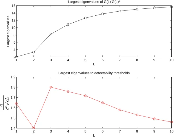
• In section 2, we consider detection Problem 1. It can be formulated as the following composite hypothesis testing problem in which the hypothesis H0 corresponds to yn = vn for n = 1,...,N and in which the hypothesis H1 corresponds to yn = [h(z)]sn+ vn for some scalar deterministic sequence s and some SIMO filter h(z) of maximal degree P − 1 where P is supposed to be known. The generalized likelihood ratio test cannot be implemented in this context because the maximum likelihood ratio estimate of s and h(z) cannot be expressed in closed form. Motivated by the GLRT in the context of narrow band signals ([12]), we thus study the reasonable pragmatic test statistics consisting in comparing the sum of the P + L − 1 largest eigenvalues of matrix ˆR(L)y to a threshold. Using the results of section 1, we study the conditions under which the above test is consistant, and discuss on the optimum value of the parameter L.
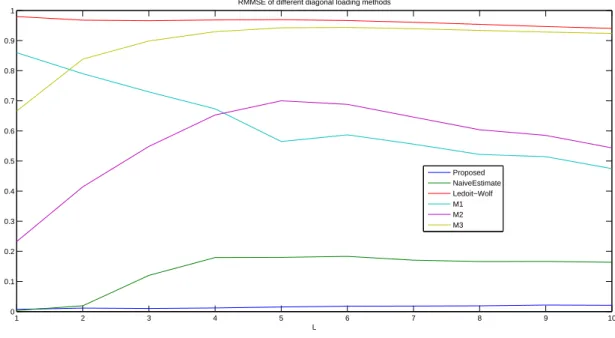
• In section 3, we consider the problem of estimating a regularized spatio-temporal Wiener filter from the observations (yn)n=1,...,Nwhen a training sequence (sn)n=1,...is available at the receiver side. The regularized spatio-temporal Wiener estimate of sequence s is defined by
ˆ
sn= ˆg(L)∗λ y(L)n
where the regularized spatio-temporal Wiener filter ˆg(L)is the ML–dimensional vector given by ˆg(L)=³Rˆ(L)y + λIML
´−1 ˆr(L)Y
where ˆr(L)Y is the empirical cross covariance between the augmented observations (y(L)n )n=1,...,Nand the training sequence (sn)n=1,...,N. Our main contribution is the derivation of a new estimation scheme of the regularization parameterλ that consists in choosing λ so as to maximize the sig-nal to noise plus interference ratio SINR(λ) provided by the regularized spatio-temporal Wiener estimate. The SINR appears to be a random variable depending on the noise samples corrupting the observations (yn)n=1,...,N. However, we prove that in the high dimension regime, it converges almost surely towards a deterministic termφ(λ), depending on λ and on the coefficients of h(z), and that can be expressed in closed form. Although the coefficients of h(z) are unknown, we prove thatφ(λ) can be estimated consistently from the observations (yn)n=1,...,Nby a term ˆφ(λ) for each λ, and we propose to choose the regularization parameter that maximizes ˆφ(λ). In order to mention the technical results that we develop, we consider the normalized matrixΣ(L) and the resolvent
Q(z) of matrixΣ(L)Σ(L)∗. Our results are based on the characterization of the asymptotic behaviour of bilinear forms of matrices Q(z), Q(z)Σ(L),Σ(L)∗Q2(z)Σ(L),Σ(L)∗Q(z)H(L)H(L)∗Σ(L)when z lies on the negative real axis. For this, we use the hypothesis that P + L − 1 does not scale with M and N, and take (1.2.31) as a starting point to express the above mentioned bilinear forms in terms of bi-linear forms of matrices depending on the resolvent QW(L)(z) of the noise part W(L)ofΣ(L)whose
behaviour is known.
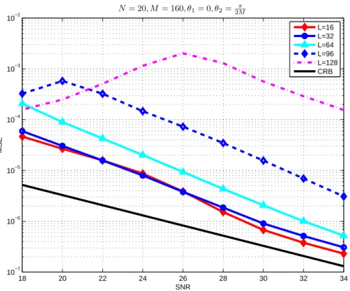
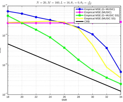
• In section 4, we address the estimation of the directions of arrival of K narrow band sources im-pinging on a large uniform linear array of sensors in the case where the number of snapshots N is large, but much smaller than the number of sensors M. In this context, it is standard to use spa-tial smoothing technics in order to generate L non overlapping subarrays of M − L + 1 sensors, and to multiply by L the number of snapshots. More precisely, the observations (yn)n=1,...,Nfollow the classical narrow band array processing model
yn= AMsn+ vn
For each n, we denote byYn(L)the (M − L + 1) × L Hankel matrix defined by Y(L) n = y1,n y2,n . . . yL,n y2,n y3,n . . . yL+1,n .. . ... ... ... ... .. . ... ... ... ... yM−L+1,n yM−L+2,n . . . yM,n (1.4.5)
Column l of matrixYn(L)corresponds to the observation on subarray l at time n. Collecting all the observations on the various subarrays allows to obtain NL snapshots, thus increasing artificially the number of observations. We define Y(L)N as the (M − L + 1) × NL block-Hankel matrix given by
Y(L)N =³Y1(L), . . . ,YN(L)´ (1.4.6) Matrix Y(L)N has a block Hankel structure similar to matrix defined by (1.4.3), the difference being that the Hankel matrices are block columns in (1.4.6) while they are block lines in (1.4.3). It is there-fore expected that the mathematical results developed to address Problems 1,2 can be used in the context of Problem 3. It is easily seen that Y(L)N is the sum of a rank K matrix whose range coincides with the space generated by the (M − L + 1)–dimensional vectors aM−L+1(θ1), . . . , aM−L+1(θK)) with
the noise matrix V(L)N defined in the same way than Y(L)N . As EÃ V (L) N V(L)∗N NL ! = σ2IM−L+1
it possible to develop consistent subspace estimation methods of the angles (θk)k=1,...,K in the asymptotic regime where NL → +∞ and M − L + 1 remains fixed. This regime corresponds to val-ues of L for which the virtual subarrays have a small number of elements, thus leading to poor resolution methods. It is thus much more relevant to address the case where M − L + 1 ' M, i.e.
L
M → 0. We thus consider an asymptotic regime in which N → +∞, M → +∞ and cN= M NL → c
where c > 0. Adapting the above mentioned results to the present context, we are able to charac-terize the largest eigenvalues and corresponding eigenvectors of the empirical covariance matrix
Y(L)N Y(L)∗N /NL provided N = O (Mβ) for 1/3 < β ≤ 1, and to deduce from this a consistent subspace estimation method of the directional parameters.
Contributions of Chapter 3. In Chapter 3, we address the case where the observation y is generated
by a general model
yn= xn+ vn
where x is a deterministic signal which is not necessarily defined as a filtered version of a scalar se-quence. In this context, matrix Y(L)= X(L)+ V(L)where X(L)is not necessarily rank deficient. In this more general context, we study the behaviour of the empirical eigenvalue distribution of normalized matrix
Σ(L)Σ(L)∗in the case where L = O (Nα) forα < 2/3. Generalizing the Gaussian tools used in [49], we prove
that the normalized traces and the bilinear forms of the resolvent Q(z) of matrixΣ(L)Σ(L)∗have the same behaviour than the normalized traces and the bilinear forms of a deterministic matrix-valued function
T(z) defined as the solution of a certain (complicated) equation. This result implies that the empirical
eigenvalue distribution ˆµNofΣ(L)Σ(L)∗has a deterministic behaviour. However, we have not been able
to characterize the properties of the corresponding deterministic approximation of ˆµN(in particular its
support), and to obtain results concerning the almost sure location of the eigenvalues ofΣ(L)Σ(L)∗. How-ever, the results of Chapter 3 are useful in Chapter 4.
Contributions of Chapter 4. In Chapter 4, we consider again the wide band model (1.4.1), but
as-sume that P and L may scale with N, and that cN=MLN converges towards a non zero constant c. We
assume that when P and L converge towards +∞, P = O (L). This implies that the rank of normalized matrix B(L)=H(L)pS(L)
N may scale with M and N, but that Rank(B
(L))/N → 0.
• In section 3 and 4, we establish that matrix T(z) can be replaced by matrix defined by (1.2.40) corre-sponding to a standard information plus noise model in which the noise matrix is i.i.d. Moreover, scalar Stieltjes transform mN(z) can also be replaced by the Stieltjes transform of the
Marcenko-Pastur with parameters (c,σ2). If more information could be obtained on the location of the eigen-values ofΣ(L)Σ(L)∗, this result could be useful to understand the behaviour of the projection ma-trices on certain eigenspaces.
• In section 5, we take benefit of the results of Chapter 3 to revisit Problem 2 in the case where P and L may converge towards +∞. In particular, using Gaussian tools, we are able to generalize the asymptotic behaviours of bilinear forms of Q(z)Σ(L),Σ(L)∗Q2(z)Σ(L) found in section 3 of Chap-ter 2 when L = O (Nα) forα < 2/3. The study of the SINR also needs to evaluate bilinear forms of
Σ(L)∗Q(z)H(L)H(L)∗Σ(L), which, in the case where P and L are fixed, is an easy task. When P and
L scale with M and N, the problem appears more difficult. We however found a satisfying result provided ML → 0 (a condition nearly equivalent to L = O (Nα) forα < 1/2) because a number of complicated terms vanish. Under this extra assumption, the SINR has the same asymptotic ex-pression than in the case where P and L are fixed. However, we feel that the asymptotic behaviour ofΣ(L)∗Q(z)H(L)H(L)∗Σ(L)could also be characterized when L = O (Nα) for 1/2 ≤ α < 2/3, and that a correcting term could appear in the expression of the limit form of the SINR.
We finally mention the publications connected to this thesis.
• G.T. Pham, P. Loubaton, P. Vallet, "Performance analysis of spatial smoothing schemes in the con-text of large arrays", IEEE Trans. on Signal Processing, vol. 64, no. 1, pp. 160-172, January 2016. • G.T. Pham, P. Loubaton, P. Vallet, "Performance analysis of spatial smoothing schemes in the
con-text of large arrays", Acoustics, Speech and Signal Processing (ICASSP), 2015 IEEE International Conference on Year: 2015, Pages: 2824 - 2828.
• G.T. Pham; P. Loubaton, "Applications of large empirical spatio-temporal covariance matrix in multipath channels detection", Signal Processing Conference (EUSIPCO), Nice, September 2015. • G.T. Pham; P. Loubaton, "Performances des filtres de Wiener spatio-temporels entrainés: le cas des
grandes dimensions", Proc. Colloque Gretsi, Lyon, September 2015.
• G.T. Pham; P. Loubaton, "Optimization of the loading factor of regularized estimated spatial-temporal Wiener filters in large system case", Proc. of Statistical Signal Processing Workshop (SSP), Palma de Majorque, June 2016.
Spatial-temporal Gaussian information
plus noise spiked model
2.1 Introduction
In this chapter, we assume that the M dimensional signals (yn)n∈Zis generated as
yn=
P−1
X
p=0
hpsn−p+ vn= [h(z)]sn+ vn (2.1.1)
where (sn)n∈Z is a non observable scalar deterministic sequence and where h(z) =PP−1p=0hpz−p is the transfer function of an unknown 1–input / M–outputs linear system. While h(z) is assumed unknown, P, which represents an upper bound on the number of non zero coefficients of h(z), is assumed to be known. (vn)n∈Zrepresents a temporally and spatially complex Gaussian white noise of varianceσ2.
In the following, we propose approaches based on the empirical spatio-temporal covariance matri-ces of y to address 3 well defined inference problems. We recall that if y(L)n is the ML–dimensional vector defined by
y(L)n = (y1,n, . . . , y1,n+L−1, . . . , yM,n, . . . , yM,n+L−1)T
then the spatio-temporal covariance matrix ˆR(L)y is the ML × ML matrix defined by ˆ R(L)y,N= 1 N N X n=1 y(L)n y(L)∗n =Y (L) N Y (L)∗ N N (2.1.2) where Y(L)N = (y(L)1 , . . . , y (L)
N ). As mentioned in Chapter 1, matrix Y (L)
N can be written as
Y(L)N = H(L)S(L)N + V(L)N (2.1.3)
where ML × (P + L − 1) matrix H(L)is the block row matrix
H(L)= H(L)1 .. . H(L)M
where each row block H(L)m is a L × (P + L − 1) Toeplitz matrix corresponding to the convolution between sequence s and the impulse response (hm,p)p=0,...,P−1 of component m hm(z) of filter h(z). In (2.1.3), (P + L − 1) × N matrix S(L)N is the Hankel matrix whose entries are defined by (S(L)N )i , j= si +j −P.