This project is funded by the European Union under the 7th Research Framework Programme (theme SSH) Grant agreement nr 290752. The views expressed in this press release do not necessarily reflect the views of the European Commission.
Working Paper n° 48
Poverty Reduction in Brazil: Changes in the Profile and in
the Determinants during the Early 2000s
UFRJ
Valeria Pero
Gabriela Freitas da Cruz
Poverty Reduction in Brazil:
Changes in the Profile and in the Determinants during the Early 2000s
1Valéria Pero2 Gabriela Freitas da Cruz3
Abstract: This article analyses the evolution of metropolitan poverty in Brazil between 2001 and 2013,
comparing it with the poverty in rural and non-metropolitan urban areas. Therefore, we will be able to identify whether poverty is becoming more urban and metropolitan and to point out the particularities of this process. Moreover, this article explores the determinants of poverty reduction through two ways: (i) the contribution of economic growth and income redistribution; and (ii) the decomposition into its direct determinants, such as access to work and to different types of income. Given the complexity and the multidimensional aspect of poverty, three poverty lines were used as a reference: (i) the official line for the Federal Government’s social programs (R$140/month in June 2011); (ii) the line based on a basket of goods and services that varies according to housing location; and (iii) the relative line, equal to 60% of the median per capita household income. The comparison of poverty rates measured by the different lines shows a generalized reduction, which is slower in relation to relative poverty than in relation to absolute poverty. The line based on the consumer basket seems more appropriate for the study of metropolitan poverty issues, since it accounts for the higher costs of living in these areas. Using this line, we observe a process of poverty metropolization: in 2013, the poverty rate in metropolitan regions was higher than the rural poverty rate. Finally, the results of the decompositions show two other important aspects: the greater contribution of income redistribution and the lesser role of other sources of income besides work, such as government cash transfers, to explain the poverty reduction in metropolitan regions if compared to rural and non-metropolitan urban areas.
Key words: poverty lines; metropolitan poverty; decomposition of poverty reduction.
1 This work is part of the Nopoor Research Project supported by the European Union (www.nopoor.eu). 2 Associate Professor at the Economics Institute of the Federal University of Rio de Janeiro (IE-UFRJ).
Email: [email protected]
3 Doctoral student in the Postgraduate Program in Economics at the Federal University of Rio de Janeiro (UFRJ).
1. INTRODUCTION
In the beginning of the 2000s Brazil was very successful in tackling poverty. The improvement in the labor market, mainly due to the increase in the minimum wage and formal employment, associated with the expansion of conditional cash transfer programs, such as the Bolsa Família, were determining factors for this picture. According to the National Household Sample Survey by the Brazilian Institute of Geography and Statistics (PNAD/IBGE), more than 25 million people left poverty between 2001 and 2013. Therefore, the poverty rate – the proportion of people living below the poverty line – decreased from 24.6% to 8.4% in this period.
Such numbers consider a poverty line equal to R$140.00 (in prices of June 2011), twice the amount of the extreme poverty line defined by the Federal Government based on Decree 7492, which created the Plano Brasil Sem Miséria (“Brazil Without Extreme Poverty Plan”). In 2001 prices, this is equivalent to R$72.74/month, and in 2013 prices, R$157.58/month (US$ 87.80 in PPP4). Therefore, they are based on very low amounts, such that the overcoming of poverty, in this case, does not necessarily involve the meeting of basic needs, especially in large metropolises where the cost of living is higher. Nevertheless, almost 17 million people were living below the poverty line in 2013, which makes evident the relevance of the theme and the existence of many challenges ahead.
The effectiveness of public policies in the war on poverty is primarily related to the comprehension of the phenomenon in its multiple dimensions, and therefore, one of the challenges is in the actual definition and measurement. Given the complexity, depending on the concept and measurement used, the dimension, the profile, and the behavior over time can vary considerably. One way of contributing to a better comprehension of the issue using the poverty rate is to consider different aspects of absolute and relative poverty (MEYER and SULIVAN, 2012; RAVALLION et al., 2007, and BELLIDO et al., 1998). In order to analyze the recent drop in the poverty rate in the rural, urban, and metropolitan areas of Brazil, three lines based on per capita household income will be used from different perspectives: (i) the official one for the Federal Government’s social programs, (ii) the one based on a minimum consumer basket, taking into account regional differences in consumption patterns and in cost of living, and (iii) the relative one, equal to 60% of median per capita household income in the area of residence.
In considering the regional dimension in the analysis, RAVALLION et al. (2007) show that the urbanization process in developing countries has contributed to the decrease in poverty, however in a lower intensity in Latin America. ROCHA (2013) analyzes data from Brazil between 1970 and 2011, and shows that, as a result of the industrialization and urbanization process and of welfare policies, poverty has also been urbanized. The more rapid decrease in the rural poverty incidence associated with urbanization has led to the gradual increase in metropolitan poverty.
Another way of analyzing poverty reduction is from its immediate macro and microeconomic determinants. In macroeconomic terms, the decrease in poverty depends on a process of development that generates an increase in income favorable to those who need more, that is, to people with lower income. BARROS et al. (2011a) estimate that between 2001 and 2008 around half of the poverty reduction in Brazil was a result of economic growth, and the other half, of the reduction in the level of inequality. Considering rural poverty between 1998 and 2005, HELFAND, ROCHA, and VINHAIS (2009) observe that its reduction occurred predominantly via economic growth. In metropolitan regions, CARNEIRO, BAGOLIN and TAI (2013) show that, despite the importance of inequality reduction, economic growth explains the greater part of poverty reduction.
In relation to microeconomic determinants, several authors (ROCHA, 2013; AZEVEDO et al., 2013; and BARROS et al., 2011b, among others) perform a per capita income decomposition based on counterfactual simulations by considering its immediate determinants, such as the employment of the
4 The conversion factor used is equal to 1.7947, the PPP (purchasing parity power) rate between R$ and US$ in September
adults in the family and the different sources of income. An estimate by BARROS et al. (2011b) points out that the growth of per capita income in the poorest 20% of the population between 2003 and 2009 was due mainly to the increase in non-labor income, which doubled in the period. However, improvements in the labor market were also expressive for this group, which recorded a growth of 40% in earned income.
With this in mind, the idea of this article is to contribute to analyzing the evolution of poverty in the 2000s, highlighting the differences among rural, urban, and metropolitan areas, and extending the analysis to a more recent period. The objectives are (i) to understand if there was in Brazil an urbanization of poverty phenomenon, commonly treated in studies on developing countries; (ii) to investigate whether, in metropolises, where inequality levels are higher than that observed in other locations, poverty reduction occurred more via growth or distribution and changes over time; and (iii) to highlight which sources of income or demographic characteristics were more relevant to the poverty reduction in various locations.
The comparison of poverty rates among the different poverty lines reveals a generalized reduction, which is slower for relative poverty than for absolute poverty. The line based on the consumer basket seems more appropriate for treating the issue of metropolitan poverty, for it takes into account differences in the cost of living among regions. According to it, a process of poverty metropolization is observed: in 2013, the poverty rate in metropolitan regions already surpassed that of rural regions. In the end, the results of the decompositions point toward two other important aspects: the greater contribution of income redistribution and the lesser importance of other non-work-related sources of income, such as government transfers, to explain the reduction of poverty in metropolises if compared to rural and urban areas.
Therefore, this article is divided into three sections, in addition to this introduction and to the conclusion. In the second section an analysis will be done of poverty measures, data sources, and decomposition methodologies. The next section presents an analysis of poverty evolution between 2001 and 2013, considering the different measures, and whether there was a recent urbanization or
metropolization process. The third section presents the results of the decompositions of poverty reduction
into its macro and microeconomic determinants. Finally, the main results are highlighted in the conclusion.
2. POVERTY MEASURES AND METHODOLOGY
2.1. Monetary Poverty Lines: Definitions and Positive and Negative Aspects
Poverty is a very complex phenomenon and its definition and measurement always carry with them the risk of limiting the analysis that one intends to do. For SEN (1999, pag. 120), “poverty should be seen as the privation of basic capabilities instead of merely as a low level of income”5. However, the
interpretation of what these basic capabilities would be is the object of intense debate and it is subject to moral values with respect to what would be the minimum acceptable to survive. Furthermore, such capabilities are related to various aspects in the life of individuals – such as healthcare, education, housing, etc. – which turn poverty into a multidimensional condition.
Even though the multidimensional character of poverty is recognized, in this article we have opted to define it based on individual incomes. This is a form of measurement that is simpler to be implemented, which demands fewer arbitrary decisions in the construction of the well-being indicator, and which facilitates the realization of the decompositions that will be performed further on. In addition, in general, monetary poverty is correlated to several individual privations, even those related to the provision of public goods and services that are not traded on the market.
After choosing income to measure individual well-being, it is necessary to establish a threshold in order to classify individuals as poor and non-poor. According to BELLIDO et al. (1998), this line can be absolute, defined by the cost of a basic consumer basket which does not vary over time, or relative, translating “a condition of relative deprivation as compared with the standard welfare of the society”
(BELLIDO et al., 1998, p. 117). With the aim of finding the line that is most adequate to the objectives of this paper, we opted to begin the analysis based on three distinct lines and choose one of them afterwards. They are: the official government poverty line, which is the same throughout Brazil; the poverty line defined on the basis of the consumer basket, which considers differences in the cost of living among regions; and the relative poverty line. The amounts of the lines are presented in Annex A.
The official extreme poverty line defined by the Federal Government in Decree nº 7492, which created the Brasil Sem Miséria Plan, and it is used as a reference for the selection of beneficiaries of the Bolsa Família Program. It is equal to R$70.006 in prices of June 2011(US$ 43.90 in September 2013
PPP). Since we are interested in poverty indicators, we adopted twice this amount (R$140.00 or US$ 87.80 in September 2013 PPP) as a threshold, a procedure that is also adopted by the Federal Government to define the amount of benefits. This amount was deflated based on the month of September (the month when the PNAD is done) every year, varying from R$72.74/month in 2001 to R$157.58/month in 2013. The fact that this line does not take into account the different costs of living in regions makes its amount represent very discrepant consumption levels throughout the country. In particular, in the metropolitan regions, where the cost of living is usually much higher, people with elevated levels of privation are not considered poor.
One way of correcting this issue is to define a basic consumer basket and calculate its cost in the different regions of the country over time. This is the methodology used by ROCHA (1997). Based on data from the 1987/88 Pesquisa de Orçamentos Familiares (“Family Budget Survey”), the author defines a consumer basket that meets the minimum nutritional criteria established by the FAO (Food and Agriculture Organization of the United Nations) in each one of the nine Brazilian metropolitan regions, Brasília, and Goiânia. The baskets of goods are different for each one of these locations, depending on the consumption patterns observed among those in the lowest income group that meets the nutritional criteria. The amount of these baskets in each one of the regions is equal to the indigence line. It is adjusted over time and calculated for other urban and rural areas in the country based on the National Consumer Price Index for food. To calculate the poverty lines, this amount is divided by the participation of these food items in income, and the sum of the money necessary to meet all of the basic needs, such as food, housing, healthcare, etc., is obtained. In 2013, the poverty lines calculated for Brazil varied from R$105.61/month in the rural area of the North region to R$398.04/month in the metropolitan region of São Paulo.
Absolute poverty lines, however, will always be marked by arbitrariness, for they require that the researcher define a basic level of consumption or income according to some criteria. Relative poverty lines, for their part, overcome this question somewhat. The line adopted by the countries of the European Union and which will be used in this paper, for example, is equal to 60% of the median income. In this case, to the extent that the country’s median standard of living increases, its poverty reference also increases. In terms of public policy, the objective is to approximate the basis of distribution to the center. In this sense, SOARES (2009) underscores that “if poverty is not based on some absolute measure, then what is measured is inequality and not poverty”7 (SOARES, 2009, p. 32). For ROCHA (1997) this type of
approach would make more sense in countries where basic needs are already met in large part. In this article, three relative lines, for each year, were calculated based on the median income of rural, non-metropolitan urban,8 and metropolitan areas in Brazil. The amounts in 2013 (excluding the rural north, which was not researched yet in the 2001 PNAD) vary between R$203.40/month in rural areas to R$420.00 in metropolitan areas. Between 2001 and 2013, in real terms, the relative poverty line became 83% higher in urban areas, 126% higher in rural areas, and 62% higher in metropolises.
6In 2014, this amount was changed to R$77.00/month. However, since this analysis goes until the year of 2013, we opted
to use the last amount that had been defined until then.
7“se a pobreza não se ancora em algum tipo de absoluto, então o que se mede é desigualdade e não pobreza”
2.2. Decomposition of Poverty Reduction Among Locations: Shift-Share Analysis
Throughout the 2000s, poverty fell in Brazil in all locations: urban, rural, and metropolitan areas. It is interesting to know, however, which location was more determinant in this process, in order to evaluate the importance of metropolitan poverty reduction in the national context. The change in poverty rate in a country is a result of both the poverty variation in each region, accounting for the share of this sub-region in the total population of the initial period, and the change in population distribution among the sub-regions, which have different poverty rates.
By following the methodology used by RAVALLION et al. (2007) to analyze poverty reduction and its possible urbanization in developing countries, it is possible to separate it into three components –urban poverty reduction, rural poverty reduction, and change in population distribution among urban and rural areas. Since we are especially interested in the issue of poverty in metropolitan areas, the decomposition performed here presents four components: rural poverty reduction, non-metropolitan urban poverty reduction, metropolitan poverty reduction, and change in population distribution among the three areas.We have, therefore, the following formula:
where is the poverty rate in period t (initial 0 or final 1) in location i (rural, urban, or metropolitan area) and is the proportion of total population that resides in location i in period t. The first three components on the right side of the equation refer to the contribution of the poverty reduction in rural, urban, and metropolitan areas, respectively, to the poverty reduction in all of Brazil. Meanwhile, the last term refers to the change in poverty resulting from the differences in population distribution among these locations along the period.
This decomposition will be performed using the three poverty lines as a reference. The comparison of its results, as well as the descriptive analysis of the data, will allow for the selection of one of these lines in order to perform the decompositions that will be described next.
2.3. Sharpley Decomposition: Decomposition of Poverty Reduction Between Growth and Distribution and Among Sources of Income
Poverty reduction occurs by means of the increase in income of the poorest people (in absolute or relative terms, depending on the line used). This increase results from both income growth for the whole population and from income redistribution from richer people to poorer people. RAVALLION and DATT
(1991) present the methodology of the decomposition of poverty reduction between two periods of time or two regions. The idea is to do a counterfactual simulation by calculating, first, the changes in poverty if income varied but distribution remained the same, and then, the changes in poverty if distribution varied but average income remained constant.
Consider a poverty measure , where z is the poverty line, is the average income in period t, and is a vector of parameters that describes the Lorentz curve9 (income distribution). By choosing the initial period as reference, we can perform the decomposition based on the following formula:
The first term between brackets is the effect of growth on changes in poverty; the second is the effect of income redistribution; and the third term is a residual that, as explained by the authors, always appears when the marginal effect of an increase in income (inequality) on poverty depends on the level of inequality (income). In general, this residual exists but, in many cases, is negligible. In the calculations made in this article, its magnitude is shown to be small, such that it is not presented in the tables.
Another type of decomposition much used in studies on poverty is presented in AZEVEDO et al. (2013). The method consists in separating the contribution of each component of income to the variation observed in the poverty indicator between two periods or regions. This type of decomposition is especially interesting in the recent period, when poverty fell considerably in developing countries. In Latin America, for example, the countries’ performance was very surprising in this sense, at a moment in which demographic changes were observed, with an increase in the proportion of the active population, significant improvements in the job market, both in terms of access and in terms of revenues, and an expansion of cash transfer programs.
By adapting the methodology presented by the authors to Brazilian data, we can define per capita household income in the following manner:
where is per capita household income; is the number of residents; is the number of adults in the household (15 years or older); is the number of employed adults; and are the sums of the work revenues and of the hours worked, respectively, of all those employed in the household; and , , and are the sums of the revenues from retirement, rent, donations from non-residents, and other incomes (government transfers and interest, in general), in this order, of all adults in the household.
The decomposition requires the construction of counterfactuals in which only one of these factors varies and the others remain constant over time. Since we are working with the individual level and lack panel data, which accompanies individuals over time, individuals are ranked according to their per capita household income, and their estimated income for the previous period is equal to the average income corresponding to their quintile in the previous period. This type of decomposition is subject to the problem known as “path-dependence,” which consists of the alteration of the results depending on the order according to which the contribution of each component is calculated. To correct this problem, the decomposition is performed by considering all of the possible orderings and the final result is the average of the results of each ordering. In the end, the authors underscore that it can be difficult to interpret these contributions as causal, for the variation of one source of income can influence the variation of another.
2.4. Data
The database used in this article was built based on microdata from the National Household Sample Survey (PNAD/IBGE) from the years 2001, 2005, 2009, and 2013. The rural area of the North region only came to be part of the survey in 2004, such that there is no available information for it in 2001. Therefore, in order to standardize the units of analysis, the rural area of the North region was excluded in all years. The descriptive results for the complete sample, with the rural North, for the years 2005 to 2013 can be seen in Annex B of this article. Brazil’s nine main metropolitan regions (Belém, Fortaleza, Recife, Salvador, Belo Horizonte, Rio de Janeiro, São Paulo, Curitiba and Porto Alegre) and the capital Brasília were considered metropolitan areas. The rest of the country was divided between (non-metropolitan) urban and rural areas according to the household location.
The calculation of per capita household income was done according to the IBGE’s standard procedure. The following were excluded from the calculation (and the database): collective households; people whose relationship to the person responsible for the household was that of pensioner, domestic worker, or relative of domestic worker; and households where one of the residents did not declare any type of income. In total, there are in the database sample between 330,000 observations in 2013 and 388,000 in 2005. Considering the observations by their respective weights, the universe of analysisvaries from around 167 million individuals in 2001 to 186 million in 2013.
Finally, the decomposition of poverty reduction according to sources of income considers that only adults have income. Therefore, it is necessary to make the following adjustments to include the income of children up to 14 years old: (i) all those responsible for the household should be considered adults, regardless of age; and (ii) the income of children up to 14 years old should be transferred to those responsible for the household, respecting the source of income. The same procedure should be done with the hours worked by them.
3. POVERTY IN THE 2000s: EVOLUTION AND DISTRIBUTION BY HOUSEHOLD LOCATION
As previously described, the distribution of poor people and non-poor people and the poverty rate according to household location (rural, urban, or metropolitan) were calculated based on three different poverty lines: i) the official poverty line; (ii) the line based on a minimum consumer basket; and (iii) the relative line. The following Table 1 presents these indicators.
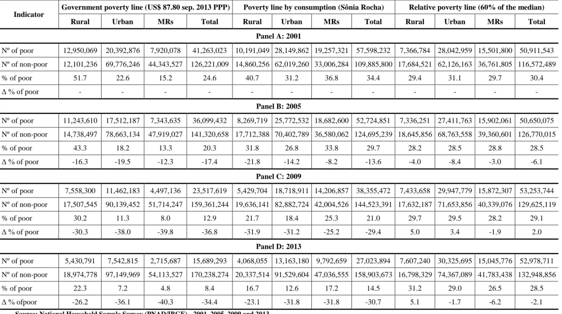
Table 1 – Number and Proportion of Poor People According to Household Location (without the Rural North): 2001 – 2013
Indicator
Government poverty line (US$ 87.80 sep. 2013 PPP) Poverty line by consumption (Sônia Rocha) Relative poverty line (60% of the median)
Rural Urban MRs Total Rural Urban MRs Total Rural Urban MRs Total
Panel A: 2001 Nº of poor 12,950,069 20,392,876 7,920,078 41,263,023 10,191,049 28,149,862 19,257,321 57,598,232 7,366,784 28,042,959 15,501,800 50,911,543 Nº of non-poor 12,101,236 69,776,246 44,343,527 126,221,009 14,860,256 62,019,260 33,006,284 109,885,800 17,684,521 62,126,163 36,761,805 116,572,489 % of poor 51.7 22.6 15.2 24.6 40.7 31.2 36.8 34.4 29.4 31.1 29.7 30.4 Δ % of poor - - - - Panel B: 2005 Nº of poor 11,243,610 17,512,187 7,343,635 36,099,432 8,269,719 25,772,532 18,682,600 52,724,851 7,336,251 27,411,763 15,902,061 50,650,075 Nº of non-poor 14,738,497 78,663,134 47,919,027 141,320,658 17,712,388 70,402,789 36,580,062 124,695,239 18,645,856 68,763,558 39,360,601 126,770,015 % of poor 43.3 18.2 13.3 20.3 31.8 26.8 33.8 29.7 28.2 28.5 28.8 28.5 Δ % of poor -16.3 -19.5 -12.3 -17.4 -21.8 -14.2 -8.2 -13.6 -4.0 -8.4 -3.0 -6.1 Panel C: 2009 Nº of poor 7,558,300 11,462,183 4,497,136 23,517,619 5,429,704 18,718,911 14,206,857 38,355,472 7,433,658 29,947,779 15,872,307 53,253,744 Nº of non-poor 17,507,545 90,139,452 51,714,247 159,361,244 19,636,141 82,882,724 42,004,526 144,523,391 17,632,187 71,653,856 40,339,076 129,625,119 % of poor 30.2 11.3 8.0 12.9 21.7 18.4 25.3 21.0 29.7 29.5 28.2 29.1 Δ % of poor -30.3 -38.0 -39.8 -36.8 -31.9 -31.2 -25.2 -29.4 5.0 3.4 -1.9 2.0 Panel D: 2013 Nº of poor 5,430,791 7,542,815 2,715,687 15,689,293 4,068,055 13,163,180 9,792,659 27,023,894 7,607,240 30,325,695 15,045,776 52,978,711 Nº of non-poor 18,974,778 97,149,969 54,113,527 170,238,274 20,337,514 91,529,604 47,036,555 158,903,673 16,798,329 74,367,089 41,783,438 132,948,856 % of poor 22.3 7.2 4.8 8.4 16.7 12.6 17.2 14.5 31.2 29.0 26.5 28.5 Δ % ofpoor -26.2 -36.1 -40.3 -34.4 -23.1 -31.8 -31.8 -30.7 5.1 -1.7 -6.2 -2.1
Using the Federal Government’s official poverty line as a reference, the number of poor people in 2001 was approximately 41 million, of which 8 million were living in metropolitan regions (MR). In 2013, the total of poor people in Brazil fell to 16 million and to 2.7 million in the metropolises. This meant a greater than 65% drop in the poverty rate both in the total and in the MR. In these, this drop was slightly higher than that of the total and the period of greatest poverty reduction happened between 2009 and 2013, while in total, the period of 2005 to 2009 was more positively significant.
Meanwhile, the poverty line calculated by ROCHA (1997), differentiated according to the cost of living in the country’s regions, also reveals a promising picture, although the increase in the threshold (in relation to the official line) in some areas results in a greater poverty rate in all of the years. The number of poor people in Brazil falls from 58 million in 2001 to around 27 million in 2013, and from 19 to 10 million in the MR. The poverty rate, for its part, falls more than 50% in all areas, from 34.4% in 2001 to 14.5% in 2013 in Brazil. On metropolitan areas, it fell from 36.8% to 17.2%, surpassing the poverty rate in rural areas, where the cost of living - and thus the poverty line - is lower.
Finally, the analysis with the relative line reveals a higher number of poor people, which remains more or less stable over time, above 50 million in the country and 15 million in the metropolises. Such stability is due to the fact that, throughout the 2000s, median income also increased a lot in Brazil, which involves a continuous increase of the line in real terms. Therefore, even though the income of the poorest people grew in the period, such growth was not enough to bring them closer to the population’s median standard of living. The poverty rate fell from 30.4% to 28.5% in Brazil, and from 29.7% to 26.5% in metropolitan regions, a much lesser performance to that observed based on the absolute poverty lines.
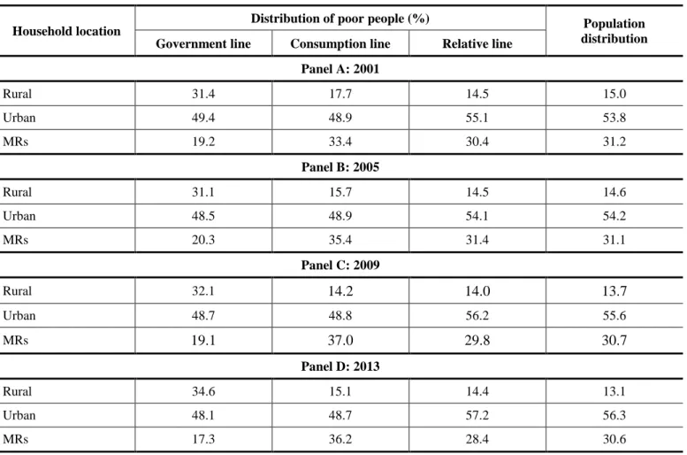
Table 2 – Distribution of Poor People and of the Population According to Household Location: 2001 – 2013
Household location
Distribution of poor people (%) Population
distribution
Government line Consumption line Relative line
Panel A: 2001 Rural 31.4 17.7 14.5 15.0 Urban 49.4 48.9 55.1 53.8 MRs 19.2 33.4 30.4 31.2 Panel B: 2005 Rural 31.1 15.7 14.5 14.6 Urban 48.5 48.9 54.1 54.2 MRs 20.3 35.4 31.4 31.1 Panel C: 2009 Rural 32.1 14.2 14.0 13.7 Urban 48.7 48.8 56.2 55.6 MRs 19.1 37.0 29.8 30.7 Panel D: 2013 Rural 34.6 15.1 14.4 13.1 Urban 48.1 48.7 57.2 56.3 MRs 17.3 36.2 28.4 30.6
Source: National Household Sample Survey (PNAD/IBGE) - 2001, 2005, 2009 and 2013.
Table 2 reveals the differences in the distribution of the poor population in the different areas and makes clearer the issue of poverty metropolization, observed only when we use the line that considers price differences among regions.
In relation to the distribution of the total population,10 a reduced proportion of inhabitants of rural regions is observed already in 2001, such that the urbanization process loses force throughout the 2000s. Actually, population distribution remains more or less stable, with a slight increase in the proportion of inhabitants of non-metropolitan urban areas and a reduction in the proportion of inhabitants of rural and metropolitan areas.
Considering poor people, their distribution depends on the poverty line used as a reference. In the case of the official line, one observes an over-representation of poor people in rural regions and a reduction in the participation of the metropolitan poor in the total of poor people, suggesting a demetropolization of poverty. Using the relative line, we obtain a distribution of poor people similar to the distribution of the total population. Finally, the methodology suggested by ROCHA (1997) is the only one to suggest a process, albeit not very accentuated, of poverty metropolization, precisely because it considers the difference in cost of living among regions. By taking into account that life in the metropolises is, in general, more expensive than in the other locations, we find a greater resistance of poverty in these areas: while the proportion of inhabitants in these areas falls between 2001 and 2013, the proportion of poor people that reside there rises from 33.4% to 36.6%. It is likely that the lower income growth in these areas as well as the fact that the Bolsa Família’s benefits are low to overcome the higher poverty line on metropolitan regions. This process, however, occurs until 2009 and seems to be reverting itself in the last period, when the proportion of poor people living in the MRs falls.
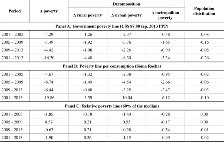
Table 3 – Shift-Share Analysis: Decomposition of Poverty Reduction According to Household Location
Period Δ poverty
Decomposition
Population distribution Δ rural poverty Δ urban poverty Δ metropolitan
poverty
Panel A: Government poverty line (US$ 87.80 sep. 2013 PPP)
2001 – 2005 -4.29 -1.26 -2.37 -0.58 -0.08
2005 – 2009 -7.49 -1.92 -3.76 -1.65 -0.16
2009 – 2013 -4.42 -1.08 -2.26 -0.99 -0.08
2001 – 2013 -16.20 -4.40 -8.30 -3.24 -0.26
Panel B: Poverty line per consumption (Sônia Rocha)
2001 – 2005 -4.67 -1.32 -2.38 -0.95 -0.02
2005 – 2009 -8.74 -1.49 -4.54 -2.66 -0.06
2009 - 2013 -6.44 -0.68 -3.25 -2.47 -0.03
2001 - 2013 -19.86 -3.59 -10.04 -6.12 -0.10
Panel C: Relative poverty line (60% of the median)
2001 - 2005 -1.85 -0.18 -1.40 -0.28 0.00
2005 - 2009 0.57 0.21 0.53 -0.17 0.00
2009 - 2013 -0.63 0.21 -0.28 -0.54 -0.01
2001 - 2013 -1.90 0.26 -1.15 -0.99 -0.02
Source: National Household Sample Survey (PNAD/IBGE) - 2001, 2005, 2009 and 2013.
10 Only people with a valid per capita household income were considered, that is, the same ones who were considered in
the calculations of poverty. The following were therefore excluded: residents of collective households; domestic workers and their relatives living in the employer’s residence; and households where one resident did not declare any type of income.
To better understand the issue of the metropolization (or not) of poverty in Brazil, Table 3 decomposes the poverty reduction according to the reduction’s contribution in each location and the contribution of the change in the population distribution among locations.
The analysis of the table above reveals that, regardless of the line considered, the redistribution of the population among the locations had a much smaller impact on poverty reduction, contrary to what other studies suggest for developing countries, such as RAVAILLON et al (2007). This result can be attributed to the advanced urbanization process in Brazil, which implies a more stable structure of population distribution among urban, rural, and metropolitan areas.
Based on the official poverty line, the poverty rate fell 16.2 percentage points between 2001 and 2013, with the greatest drop between 2005 and 2009. In all periods, the drop in metropolitan poverty was that which least contributed to the drop in poverty in Brazil, even with the share of its population in total being close to one third. In large part, this result can be explained by the fact that poverty in metropolitan areas is less than in others, such that, in terms of percentage points, its drop is always less. Urban areas, for their part, were the ones which most contributed, both due to the good performance in these small and medium-sized cities, and due to their higher share in the country’s total population.
Considering the line defined by the basic consumer basket, the poverty reduction was greater, of 19.9 percentage points. The reduction in non-metropolitan areas was the most responsible for this result, while the reduction in rural areas had the least participation. Again, a better performance is observed in the period from 2005 to 2009.
Meanwhile, the relative poverty line points to a much lesser poverty reduction, of 1.9 percentage points. Between 2005 and 2009, the period of greatest growth in the Brazilian economy in the 2000s, the poverty rate according to this line increases; meanwhile, in rural areas, it rises in the whole period. It seems, therefore, that the high economic growth observed over these years has not been so favorable to the poorest people, especially those who live in the countryside. What is observed based on this data is that they have been raising their income level, but not enough to catch up with the growing level of median income on the growing level of median income.
Taking into account the analysis performed and the objective proposed, to investigate the evolution of poverty in the 2000s with a focus on metropolitan areas, the poverty line established based on a minimum consumption standard was considered more adequate. This line considers a factor that is essential for treating the issue: although access to public goods and infrastructure is greater in big cities, which contributes to the alleviation of the poverty situation, the cost of living is much higher in these areas. This reduces the consumption standard of the poorest people and makes government cash transfer policies insufficient to guarantee of the most basic needs. The use of this type of poverty line is also in accordance with some results of international studies with respect to ways of identifying the neediest individuals in terms of access to goods and services. MEYER and SULLIVAN (2012), for example, compare the poorest individuals in the United States according to three criteria: the government’s official line, which considers gross family income; the measurement of supplemental poverty, which considers available income and makes other adjustments; and family consumption. The authors’ conclusion is that the measuring of family well-being through consumption indicators better meets the objective of identifying those who really have greater privations.
4. DECOMPOSITION OF POVERTY REDUCTION IN THE 2000s
4.1. Growth and Income Distribution
Poverty reduction can happen in two ways: total income growth, for all social strata; and income redistribution, from the richest to the poorest. The following Table 4 presents the evolution of average per capita household income in the period, and of the Gini index, which measures the inequality in the distribution of this income among individuals. The amounts were all deflated by using as a reference the same deflators of the consumption poverty line, which are differentiated among the various regions.
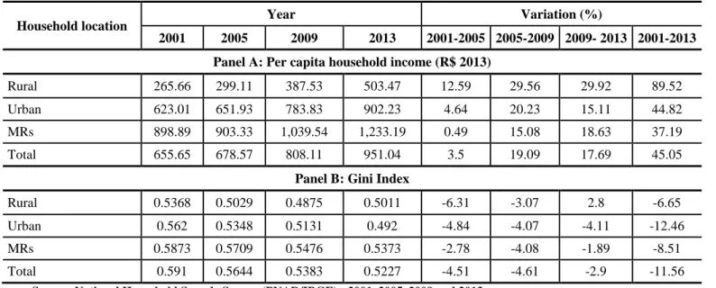
Table 4 – Descriptive Analysis: Growth x Inequality
Household location Year Variation (%)
2001 2005 2009 2013 2001-2005 2005-2009 2009- 2013 2001-2013
Panel A: Per capita household income (R$ 2013)
Rural 265.66 299.11 387.53 503.47 12.59 29.56 29.92 89.52
Urban 623.01 651.93 783.83 902.23 4.64 20.23 15.11 44.82
MRs 898.89 903.33 1,039.54 1,233.19 0.49 15.08 18.63 37.19
Total 655.65 678.57 808.11 951.04 3.5 19.09 17.69 45.05
Panel B: Gini Index
Rural 0.5368 0.5029 0.4875 0.5011 -6.31 -3.07 2.8 -6.65
Urban 0.562 0.5348 0.5131 0.492 -4.84 -4.07 -4.11 -12.46
MRs 0.5873 0.5709 0.5476 0.5373 -2.78 -4.08 -1.89 -8.51
Total 0.591 0.5644 0.5383 0.5227 -4.51 -4.61 -2.9 -11.56
Source: National Household Sample Survey (PNAD/IBGE) - 2001, 2005, 2009 and 2013.
The period from 2001 to 2013 was marked by a strong growth of family income (45% in total), especially after 2005. A larger growth in rural areas (90%) and a smaller variation in metropolitan regions (31%) were observed, reducing the regional differences. Inequality, for its part, fell in all locations and also in country as whole: the Gini index fell from 0.591 in 2001 to 0.523 in 2013 (-12%), especially in the period from 2005-2009 and in urban areas. In rural areas, for their part, inequality reduction was lower, and even increased between 2009 and 2013. During the whole period, a greater inequality in metropolises was observed than in other areas.
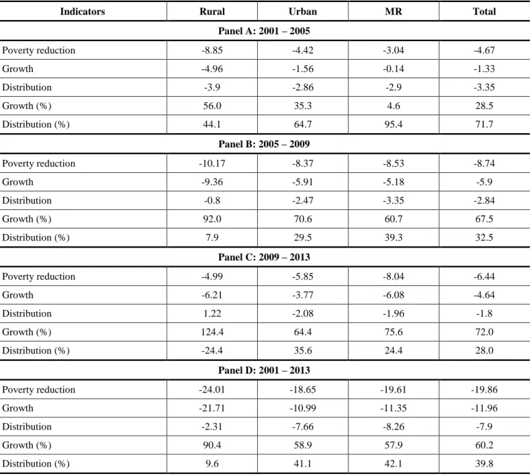
Table 5 presents the decomposition of changes in poverty into two components: average per capita income growth and income inequality changes. Between 2001 and 2013, both growth and income redistribution contributed to poverty reduction. The former, however, was more important, especially in rural areas, where it was responsible for 90% of the drop observed in the poverty rate. In metropolitan regions, income redistribution, although less relevant than growth, was more important than in other locations, accounting for 42% of the poverty reduction.
By analyzing the decomposition of the sub-periods, we can observe that between 2001 and 2005, a period of lower growth, redistribution was the most significant determinant for the reduction in the poverty rate, mainly in the MR, where growth contributed with only 5%. Throughout the periods, we see an increase of the contribution of economic growth to poverty reduction. Between 2009 and 2013, growth had the greatest contribution of the sub-periods, possibly because, in these years, the income redistribution process underwent a strong deceleration.
The data shows, therefore, that poverty reduction was greater in periods of greater growth and not of greater redistribution. The former was the most responsible for the favorable evolution of this indicator in the period as a whole. Even in metropolitan regions, where redistribution had a more relevant role than in other areas, growth was the main determinant of poverty reduction. It can be worrisome, keeping in mind the stagnation of income inequality in the most recent period and the prospects of recession in the Brazilian economy in the years to come.
Table 5 – Decomposition of Poverty Reduction – Consumption Line: Growth x Distribution
Indicators Rural Urban MR Total
Panel A: 2001 – 2005 Poverty reduction -8.85 -4.42 -3.04 -4.67 Growth -4.96 -1.56 -0.14 -1.33 Distribution -3.9 -2.86 -2.9 -3.35 Growth (%) 56.0 35.3 4.6 28.5 Distribution (%) 44.1 64.7 95.4 71.7 Panel B: 2005 – 2009 Poverty reduction -10.17 -8.37 -8.53 -8.74 Growth -9.36 -5.91 -5.18 -5.9 Distribution -0.8 -2.47 -3.35 -2.84 Growth (%) 92.0 70.6 60.7 67.5 Distribution (%) 7.9 29.5 39.3 32.5 Panel C: 2009 – 2013 Poverty reduction -4.99 -5.85 -8.04 -6.44 Growth -6.21 -3.77 -6.08 -4.64 Distribution 1.22 -2.08 -1.96 -1.8 Growth (%) 124.4 64.4 75.6 72.0 Distribution (%) -24.4 35.6 24.4 28.0 Panel D: 2001 – 2013 Poverty reduction -24.01 -18.65 -19.61 -19.86 Growth -21.71 -10.99 -11.35 -11.96 Distribution -2.31 -7.66 -8.26 -7.9 Growth (%) 90.4 58.9 57.9 60.2 Distribution (%) 9.6 41.1 42.1 39.8
Source: National Household Sample Survey (PNAD/IBGE) - 2001, 2005, 2009 and 2013.
4.2. Sources of Income
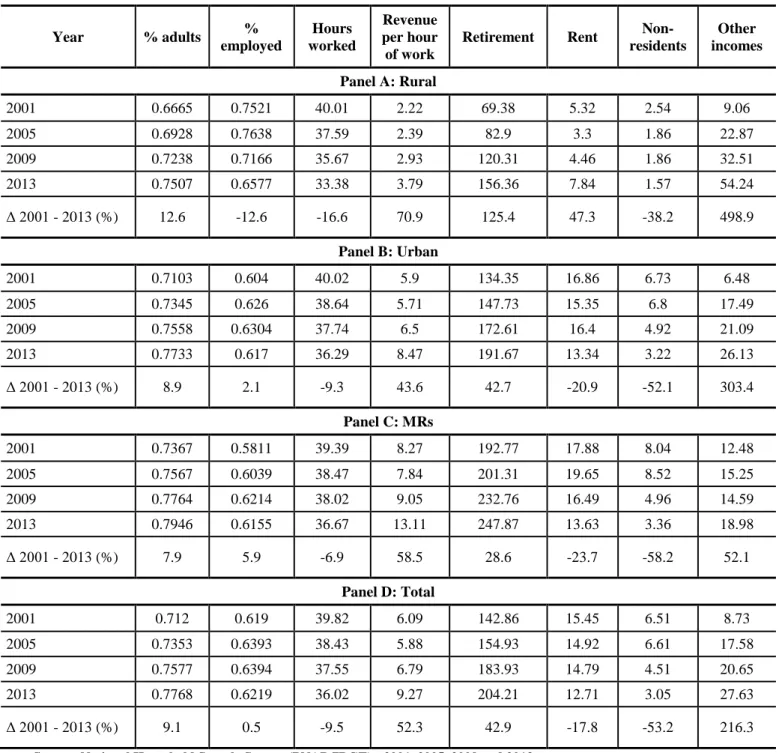
Families have several sources of revenue and each of them can be more or less important for overcoming poverty in different periods. Demographic factors can also contribute to poverty reduction: the greater the proportion of adults in the family, the greater the possibility of obtaining income and the lesser the proportion of dependents. In addition, the economy’s employment rate is also relevant, keeping in mind that work income is usually the main source of family income. The following Table 6 presents the average of the various sources of income, all in terms of per capita household income (total incomes from a particular source in the household/number of adults or number of employed, in the case of labor income). For adults who did not have a particular type of income, this income was considered equal to zero.
Table 6 – Descriptive Analysis: Sources of Income Year % adults % employed Hours worked Revenue per hour of work
Retirement Rent
Non-residents Other incomes Panel A: Rural 2001 0.6665 0.7521 40.01 2.22 69.38 5.32 2.54 9.06 2005 0.6928 0.7638 37.59 2.39 82.9 3.3 1.86 22.87 2009 0.7238 0.7166 35.67 2.93 120.31 4.46 1.86 32.51 2013 0.7507 0.6577 33.38 3.79 156.36 7.84 1.57 54.24 Δ 2001 - 2013 (%) 12.6 -12.6 -16.6 70.9 125.4 47.3 -38.2 498.9 Panel B: Urban 2001 0.7103 0.604 40.02 5.9 134.35 16.86 6.73 6.48 2005 0.7345 0.626 38.64 5.71 147.73 15.35 6.8 17.49 2009 0.7558 0.6304 37.74 6.5 172.61 16.4 4.92 21.09 2013 0.7733 0.617 36.29 8.47 191.67 13.34 3.22 26.13 Δ 2001 - 2013 (%) 8.9 2.1 -9.3 43.6 42.7 -20.9 -52.1 303.4 Panel C: MRs 2001 0.7367 0.5811 39.39 8.27 192.77 17.88 8.04 12.48 2005 0.7567 0.6039 38.47 7.84 201.31 19.65 8.52 15.25 2009 0.7764 0.6214 38.02 9.05 232.76 16.49 4.96 14.59 2013 0.7946 0.6155 36.67 13.11 247.87 13.63 3.36 18.98 Δ 2001 - 2013 (%) 7.9 5.9 -6.9 58.5 28.6 -23.7 -58.2 52.1 Panel D: Total 2001 0.712 0.619 39.82 6.09 142.86 15.45 6.51 8.73 2005 0.7353 0.6393 38.43 5.88 154.93 14.92 6.61 17.58 2009 0.7577 0.6394 37.55 6.79 183.93 14.79 4.51 20.65 2013 0.7768 0.6219 36.02 9.27 204.21 12.71 3.05 27.63 Δ 2001 - 2013 (%) 9.1 0.5 -9.5 52.3 42.9 -17.8 -53.2 216.3
Source: National Household Sample Survey (PNAD/IBGE) - 2001, 2005, 2009 and 2013.
The proportion of adults in households rose in the period, as a result of the demographic transition through which Brazil has been passing. Such a process is already found in a more advanced stage in MRs, which present a proportion of adults per household greater than that of other areas during the whole period. This greater proportion of adults implies more opportunities of income generation within the family, such that the concept of demographic bonus, in general thought of in macroeconomic terms, can also be applied to household units. The proportion of employed adults, for its part, grows until 2009 and falls since then, reflecting the deceleration of new job creation in the Brazilian economy in the last few years. In rural areas, this indicator has already fallen since 2005, possibly due to the liberation of the agricultural work force in light of the sector’s mechanization. The employment rate was lower in metropolitan regions during the whole period, but, in compensation, it was in these areas where it most increased.
In all locations, the average of hours worked fell. Revenue/hour, for its part, increased considerably (52% in total, between 2001 and 2013). The largest growth was observed in rural areas, while the smallest
was observed in urban areas. The average retirement income also had a strong growth (43% in total, between 2001 and 2013), both due to the real increase in the value of benefits, and due to the increase in the proportion of adults who receive them. The growth was particularly expressive in rural areas (125%) and less intense in MRs. Finally, incomes classified as “other incomes” – which include mainly social benefits, such as the Bolsa Família, and interest revenues – had the largest increase in the period (216%). The growth was less expressive in metropolitan areas, while in urban areas, the average of other incomes was multiplied by four, and in rural areas, by six. Again, this increase is a result both of the growth in coverage of social benefits, and of their amounts.
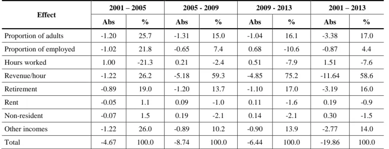
In order to better delimit the contribution of each component to poverty reduction, we made a decomposition, whose results are presented in tables 7A and 7B. Analyzing the results from Brazil as a whole (Table 7B), we observe a very large and growing importance of the real increase of revenue per hour worked (it explains 59% of the poverty reduction between 2001 and 2013), especially in the last sub-period. The average of hours worked, for its part, contributed negatively, since it decreased over time. Meanwhile, retirement revenue contributed with 14% and other revenues, such as government cash transfers, with 16%. It is significant that, between 2001 and 2005, when income increased much less, the proportion of adults, a demographic factor, and other incomes were the most important determinants of poverty rate reduction. Finally, between 2009 and 2013, the employment rate fell, acting in the opposite direction of the poverty reduction.
In relation to the analysis by location (Table 7A), it is significant the fact that, in MRs, other incomes contributed much less than to the country total (5.6%). It is probably a result of the correction of the poverty lines by the price index: since the lines in metropolises are higher, federal social benefits (the same for all regions in Brazil) were not enough to take people out of poverty. Between 2001 and 2005, revenue/hour fell in MRs, contributing in a negative way to the war on poverty. On the other hand, the proportion of adults and employed had the largest positive contributions. Meanwhile, between 2009 and 2013 revenue/hour had a positive contribution of 76% more than that observed for the country total.
In rural areas, for their part, retirement revenues and other revenues were much more relevant for poverty reduction than in the rest of the country, demonstrating the dependence of these areas in relation to social benefits. Between 2009 and 2013, for example, other revenues contributed with 73% of the poverty reduction. Finally, in urban areas, a large importance of these other revenues is observed in the period from 2001 to 2005 (27%).
Table 7A–Decomposition of Poverty Reduction – Consumption Line: Sources of Income (Urban, Rural, Metropolitan)
Effect
2001 – 2005 2005 – 2009 2009 - 2013 2001 – 2013
Abs % Abs % Abs % Abs %
Rural Proportion of adults -1.82 20.6 -1.96 19.2 -1.18 23.6 -4.57 19.0 Proportion of employed -0.74 8.3 1.05 -10.3 1.91 -38.2 2.10 -8.7 Hours worked 1.57 -17.7 0.82 -8.0 1.35 -26.9 2.95 -12.3 Revenue/hour -4.13 46.6 -5.40 53.1 -2.28 45.7 -11.23 46.7 Retirement -1.03 11.7 -2.30 22.6 -1.24 24.9 -4.99 20.8 Rent -0.08 0.9 -0.02 0.2 0.03 -0.7 0.01 0.0 Non-resident 0.02 -0.2 0.00 0.0 0.07 -1.5 0.10 -0.4 Other incomes -2.64 29.8 -2.35 23.1 -3.65 73.1 -8.38 34.9 Total -8.85 100.0 -10.17 100.0 -4.99 100.0 -24.01 100.0 Urban Proportion of adults -1.07 24.1 -1.08 12.9 -0.88 15.1 -2.86 15.3 Proportion of employed -1.05 23.8 -0.60 7.2 0.69 -11.7 -0.83 4.5 Hours worked 1.16 -26.3 0.30 -3.5 0.44 -7.5 1.46 -7.8 Revenue/hour -1.48 33.4 -4.84 57.7 -4.43 75.6 -11.07 59.4 Retirement -0.72 16.2 -1.26 15.0 -0.93 15.8 -2.80 15.0 Rent -0.05 1.1 -0.03 0.4 0.05 -0.8 0.06 -0.3 Non-resident -0.03 0.7 0.08 -1.0 0.07 -1.2 0.18 -1.0 Other incomes -1.20 27.0 -0.95 11.3 -0.86 14.6 -2.79 15.0 Total -4.42 100.0 -8.37 100.0 -5.85 100.0 -18.65 100.0 MRs Proportion of adults -1.10 36.1 -1.24 14.5 -1.29 16.0 -3.63 18.5 Proportion of employed -1.31 43.2 -1.56 18.3 -0.02 0.3 -2.84 14.5 Hours worked 0.63 -20.6 0.06 -0.7 0.47 -5.8 1.05 -5.3 Revenue/hour 0.33 -10.8 -4.91 57.5 -6.13 76.2 -10.86 55.4 Retirement -0.85 28.0 -0.88 10.3 -1.14 14.1 -2.80 14.3 Rent -0.07 2.4 0.14 -1.6 0.15 -1.9 0.26 -1.3 Non-resident -0.09 2.8 0.19 -2.3 0.18 -2.3 0.32 -1.6 Other incomes -0.57 18.8 -0.33 3.9 -0.27 3.4 -1.10 5.6 Total -3.04 100.0 -8.53 100.0 -8.04 100.0 -19.62 100.0
Table 7B – Decomposition of Poverty Reduction – Consumption Line: Sources of Income (Total)
Effect
2001 – 2005 2005 - 2009 2009 - 2013 2001 – 2013
Abs % Abs % Abs % Abs %
Proportion of adults -1.20 25.7 -1.31 15.0 -1.04 16.1 -3.38 17.0 Proportion of employed -1.02 21.8 -0.65 7.4 0.68 -10.6 -0.87 4.4 Hours worked 1.00 -21.3 0.21 -2.4 0.51 -7.9 1.51 -7.6 Revenue/hour -1.22 26.2 -5.18 59.3 -4.85 75.2 -11.64 58.6 Retirement -0.89 19.0 -1.20 13.7 -1.10 17.0 -3.19 16.0 Rent -0.05 1.1 0.09 -1.0 0.11 -1.6 0.19 -0.9 Non-resident -0.07 1.5 0.19 -2.1 0.14 -2.1 0.30 -1.5 Other incomes -1.22 26.0 -0.89 10.2 -0.90 13.9 -2.77 14.0 Total -4.67 100.0 -8.74 100.0 -6.44 100.0 -19.86 100.0
Source: National Household Sample Survey (PNAD/IBGE) - 2001, 2005, 2009 and 2013.
5. CONCLUSION
Few socioeconomic indicators are so observed and important for public policy as the poverty rate. It is a measurement used to express the percentage of people living in privation, being, therefore, fundamental to determine the well-being of society. The pursuit of the eradication of poverty, in addition to the ethical imperative, is the objective of social programs that involve a significant volume of resources from the public sector. Therefore, to comprehend the poverty phenomenon in its complexity requires entering conceptual issues that involve different measures to capture changes over time.
For this purpose, we analyzed three poverty rates and observed that there was a generalized reduction of poverty considering the period from 2001 to 2013. However, the intensity varies according to the measure and to the area of residence. When the relative poverty rate (60% of median income) is analyzed, we observe that poverty rate decreased more slowly, a much lesser performance than that observed based on absolute poverty lines. The greatest poverty rate reduction in Brazil occurred on the basis of the Federal Government’s official poverty line. Meanwhile, using the poverty line differentiated according to the cost of living between country’s regions, it is worth highlighting that the poverty rate in 2013 in metropolises comes to be greater than in rural areas, where the cost of living is lower, and consequently, the poverty line as well.
Indeed, by comparing the distribution of the poor population among rural, urban, and metropolitan areas according to different poverty lines, the issue of poverty metropolization becomes clear only when we use the consumption line. However, the decomposition results reveal that, regardless of the line considered, the population redistribution among the locations had a much smaller impact on poverty reduction, contrary to what other studies suggest for developing countries. This result can be attributed to Brazil’s advanced urbanization process in the second millennium, which involves a more stable structure of population distribution among urban, rural, and metropolitan areas.
The decomposition of changes in poverty into its macro determinants, economic growth and income redistribution, show that in the beginning of the period of analysis (2001-2005), income redistribution contributed much to diminish poverty rate, especially in metropolitan regions. However, this component loses its explanatory power over time. In addition, poverty reduction was greater in periods of greater growth, this being the most responsible for the favorable evolution of this indicator in the period as a whole. Even in metropolitan regions, where redistribution had a more relevant role than in other areas, income growth became the main determinant of this process. This is a result that points toward the necessity of persisting on the path of inequality reduction, since there is still room to redistribute income,
in order to strengthen the effects of growth in favorable moments and keep fighting poverty even in periods of economic deceleration.
Finally, the decomposition of poverty reduction in Brazil into its immediate microeconomic determinants reveals that a large and growing part of it is explained by the growth of revenue per hour worked (it explains 59% of the poverty reduction between 2001 and 2013). Meanwhile, retirement revenue contributed with 14% and other revenues, such as government cash transfers, with 16%. It is significant that in metropolitan regions the other incomes contributed much less than to the country total (5.6%). In rural areas, for their part, retirement revenues and other revenues were much more relevant for diminishing poverty than in the rest of the country, demonstrating the dependence of these areas in relation to social benefits. Between 2009 and 2013, for example, other revenues contributed with 73% of the poverty reduction. Finally, in urban areas, a large importance of these other revenues is observed in the period from 2001 to 2005 (27%).
In short, the adoption of a line differentiated among the country’s regions was shown to be fundamental for capturing the specificities of poverty in the metropolises. If, on the one hand, the poor people in metropolitan regions have, in general, greater access to public goods and services – such as education, healthcare, basic sanitation, etc. – on the other hand, the maintenance of a basic standard of consumption depends on a higher income level. Based on a poverty line differentiated among the regions, what is observed is that poverty fell less in metropolitan regions between 2001 and 2009 than in rural and urban regions. In the period from 2009 to 2013, the performance in these areas was greater, but this was not enough to avoid the poverty rate in metropolitan regions surpassing that observed in rural and urban areas in 2013. It seems, therefore, that there is a process of poverty metropolization in Brazil, albeit not very accelerated, pointing out the need for specific public policies for these areas.
The decompositions of the determinants point to important conclusions for explaining the smaller poverty reduction in metropolitan areas. On the one hand, income redistribution loses its explanatory power over time, and in the period as a whole, economic growth was the main determinant of changes in poverty. On the other hand, the decomposition by sources of income demonstrates the lesser efficacy of cash transfer programs and a greater dependence of these areas in relation to employment performance. Faced with a prospect of low growth and of an increase in unemployment in the next few years, therefore, metropolitan regions tend to be affected even more, since the social programs that are fundamental for securing income stability in times of crisis seem less effective in meeting the needs of those who live there. Changing this perspective is possible and requires an effort to promote public policies that are more effective on improving access to more and better work and income opportunities for the poorest people.
BIBLIOGRAPHICAL REFERENCES
AZEVEDO, J. P. et al. Is labor income Responsible for poverty reduction? A decomposition approach.
World Bank, Policy Research Working Paper, nº 6414. Apr., 2013.
BARRETO, F. A.; FRANÇA, J. M.; OLIVEIRA, V.H. O que mais importa no combate a pobreza,
crescimento da renda ou redução da desigualdade? Evidências para as regiões brasileiras. Fortaleza,
CE: UFC/CAEN/LEP, 2008. (Ensaio sobre pobreza, 16).
BARROS et al. Sobre a evolução recente da pobreza e da desigualdade no Brasil. In: CASTRO, J. A., VAZ, F. M. (orgs.) Situação social brasileira: monitoramento das condições de vida 1. IPEA. 2011. BARROS, R. P.; MENDONÇA, R.; TSUKADA, R. Portas de saída, inclusão produtiva e erradicação da extrema pobreza no Brasil. Chamada para Debate, Texto para Discussão, Secretaria de Assuntos
Estratégicos. Aug., 2011(b).
BELLIDO, N. P. et al. The measurement and analysis of poverty and inequality: an application to Spanish conurbations. International Statistical Review, v. 66, nº 1. Apr, 1998.
BRASIL. Decree nº 7.492, June 2, 2011. It creates the Brasil Sem Miséria Plan. Diário Oficial da União, Brasília, DF, Jun. 3, 2013.
CARNEIRO, D. M., BAGOLIN, I. P., TAI, S. H. T. Determinantes da pobreza nas regiões metropolitanas do Brasil no período de 1995 a 2009. Anais do XVI Encontro de Economia da Região
Sul - ANPEC SUL 2013.Curitiba: Jun., 2013.
HELFAND, S. M., ROCHA, R., VINHAIS, H. E. F. Pobreza e desigualdade de renda no Brasil rural: uma análise da queda recente. Pesquisa e Planejamento Econômico, v. 39, nº 1. Apr., 2009
MEYER, B. D., SULLIVAN, J. X. Identifying the disadvantaged: official poverty, consumption poverty, and the new supplemental poverty measure. The Journal of Economic Perspectives, v. 26, nº 3. 2012. RAVALLION, M., CHEN, S., SANGRAULA, P. New evidence on the urbanization of global poverty.
Population and Development Review, v. 33, nº. 4. Dec., 2007.
RAVALLION, M., DATT, G. Growth and redistribution components of changes in poverty measures: a decomposition with applications to Brazil and India in the 1980s. World Bank, LSMS Working Paper, nº 83. 1991.
ROCHA, S. Do consumo observado à linha de pobreza. Pesquisa e Planejamento Econômico, v. 27, nº 2. Aug., 1997.
ROCHA, S. Pobreza no Brasil: a evolução de longo prazo (1970-2011). Estudos e pesquisa, nº 42. XXV Fórum Nacional (Jubileu de Prata – 1988/2013) O Brasil de Amanhã. Transformar Crise em Oportunidade. May., 2013.
SEN, A.Desenvolvimento como liberdade. São Paulo: Companhia das Letras, 1999.
SOARES, S. S. D. Metodologias para estabelecer a linha de pobreza: objetivas, subjetivas, relativas, multidimensionais. IPEA, Texto para Discussão, nº 1381. Feb., 2009.
ANNEX A: POVERTY LINES
ANNEX A1 – Government Poverty Line (R$ 140.00 in June 2011)
Year Line (R$)
2001 72.74
2005 104.20
2009 125.73
2013 157.58
ANNEX A2 – Relative Poverty Line (60% of the Median Line)
Year Household location Line with rural North (R$) Line without rural North
(R$) 2001 Rural - 42.00 2001 Urban - 93.60 2001 MRs - 121.20 2005 Rural 73.05 73.71 2005 Urban 150.00 150.00 2005 MRs 180.00 181.20 2009 Rural 120.75 123.75 2009 Urban 235.80 235.80 2009 MRs 279.00 279.00 2013 Rural 192.60 203.40 2013 Urban 366.72 366.72 2013 MRs 420.00 420.00
ANNEX A3–Consumption Poverty Line (Sônia Rocha)
Regions and Strata 2001 (R$) 2005 (R$) 2009 (R$) 2013 (R$)
North Belém 103.65 151.37 190.36 241.52 Urban 90.35 131.95 165.93 210.53 Rural - 66.19 83.24 105.61 Northeast Fortaleza MR 100.60 146.61 177.73 229.25 Recife MR 146.12 212.02 264.81 336.09 Salvador MR 132.95 187.58 235.67 296.09 Urban 89.30 128.47 159.52 202.61 Rural 53.86 77.49 96.22 122.21
Minas Gerais/Espírito Santo
Belo Horizonte MR 126.10 186.35 231.92 294.41 Urban 84.78 125.29 155.92 197.93 Rural 50.19 74.17 92.30 117.17 Rio de Janeiro Metropolis 150.80 218.44 265.65 338.04 Urban 93.82 135.91 165.29 210.33 Rural 68.49 99.21 120.66 153.54 São Paulo Metropolis 188.04 261.60 316.39 398.04 Urban 120.16 167.16 202.17 254.35 Rural 75.59 105.16 127.19 160.01 Sul Curitiba MR 124.13 173.59 205.34 264.22 Porto Alegre MR 96.20 138.38 168.51 209.53 Urban 82.73 117.15 140.38 177.89 Rural 55.78 78.98 94.64 119.93 Mid-West Brasília 171.44 251.57 308.12 384.64 Goiânia 159.64 234.81 289.07 357.13 Urban 121.55 178.79 220.10 271.92 Rural 69.81 102.68 126.41 156.17
ANNEX B: NUMBER AND PROPORTION OF POOR PEOPLE, WITH RURAL NORTH: 2005 – 2013
ANNEX B1–Number and Proportion of Poor People According to Household Location (with Rural North): 2005 – 2013
Indicator
Government poverty line (US$ 87.80 sep. 2013 PPP) Consumption poverty line (Sônia Rocha) Relative poverty line (60% of the median)
Rural Urban MRs Total Rural Urban MRs Total Rural Urban MRs Total
Panel A: 2005 Nº of poor 13,132,690 17,512,187 7,370,191 38,015,068 9,185,380 25,772,532 18,722,877 53,680,789 8,345,641 27,411,763 15,610,419 51,367,823 Nº of non-poor 17,008,008 78,663,134 47,952,247 143,623,389 20,955,318 70,402,789 36,599,561 127,957,668 21,795,057 68,763,558 39,712,019 130,270,634 % of poor 43.6 18.2 13.3 20.9 30.5 26.8 33.8 29.6 27.7 28.5 28.2 28.3 Δ % of poor - - - - Panel B: 2009 Nº of poor 8,870,958 11,462,183 4,513,415 24,846,556 5,990,138 18,718,911 14,233,617 38,942,666 8,468,523 29,947,779 15,916,237 54,332,539 Nº of non-poor 20,383,837 90,139,452 51,762,860 162,286,149 23,264,657 82,882,724 42,042,658 148,190,039 20,786,272 71,653,856 40,360,038 132,800,166 % of poor 30.3 11.3 8.0 13.3 20.5 18.4 25.3 20.8 28.9 29.5 28.3 29.0 Δ % of poor -30.4 -38.0 -39.8 -36.6 -32.8 -31.2 -25.3 -29.6 4.5 3.4 0.2 2.7 Panel C: 2013 Nº of poor 6,617,951 7,542,815 2,723,269 16,884,035 4,720,883 13,163,180 9,811,614 27,695,677 8,559,990 30,325,695 15,091,045 53,976,730 Nº of non-poor 21,977,566 97,149,969 54,166,156 173,293,691 23,874,634 91,529,604 47,077,811 162,482,049 20,035,527 74,367,089 41,798,380 136,200,996 % of poor 23.1 7.2 4.8 8.9 16.5 12.6 17.2 14.6 29.9 29.0 26.5 28.4 Δ % of poor -23.7 -36.1 -40.3 -33.1 -19.4 -31.8 -31.8 -30.0 3.4 -1.7 -6.2 -2.2
Scientific Coordinator : Xavier Oudin ([email protected]) Project Manager : Delia Visan ([email protected])
Find more on www.nopoor.eu Visit us on Facebook, Twitter and LinkedIn