GOCE: precise orbit determination for the entire mission

DOI 10.1007/s00190-014-0742-8 O R I G I NA L A RT I C L E

GOCE: precise orbit determination for the entire mission

Ulrich Meyer

Received: 18 February 2014 / Accepted: 7 June 2014 / Published online: 2 July 2014 © Springer-Verlag Berlin Heidelberg 2014

Abstract The Gravity field and steady-state Ocean Circu-lation Explorer (GOCE) was the first Earth explorer core mission of the European Space Agency. It was launched on March 17, 2009 into a Sun-synchronous dusk-dawn orbit and re-entered into the Earth’s atmosphere on November 11, 2013. The satellite altitude was between 255 and 225 km for the measurement phases. The European GOCE Gravity consortium is responsible for the Level 1b to Level 2 data processing in the frame of the GOCE High-level processing facility (HPF). The Precise Science Orbit (PSO) is one Level 2 product, which was produced under the responsibility of the Astronomical Institute of the University of Bern within the HPF. This PSO product has been continuously delivered dur-ing the entire mission. Regular checks guaranteed a high con-sistency and quality of the orbits. A correlation between solar activity, GPS data availability and quality of the orbits was found. The accuracy of the kinematic orbit primarily suffers from this. Improvements in modeling the range corrections at the retro-reflector array for the SLR measurements were made and implemented in the independent SLR validation for the GOCE PSO products. The satellite laser ranging (SLR) validation finally states an orbit accuracy of 2.42 cm for the kinematic and 1.84 cm for the reduced-dynamic orbits over the entire mission. The common-mode accelerations from the GOCE gradiometer were not used for the official PSO product, but in addition to the operational HPF work a study was performed to investigate to which extent common-mode accelerations improve the reduced-dynamic orbit determina-tion results. The accelerometer data may be used to derive realistic constraints for the empirical accelerations estimated for the reduced-dynamic orbit determination, which already

H. Bock (

B

Astronomical Institute of the University of Bern, Sidlerstrasse 5, 3012 Bern, Switzerland

e-mail: [email protected]

improves the orbit quality. On top of that the accelerom-eter data may further improve the orbit quality if realistic constraints and state-of-the-art background models such as gravity field and ocean tide models are used for the reduced-dynamic orbit determination.

Keywords GOCE· Precise orbit determination · GPS · Accelerometer· SLR · Solar activity

1 Introduction

The Gravity field and steady-state Ocean Circulation Explorer (Floberghagen et al. 2011, GOCE) was the first Earth explorer core mission of the Living Planet Programme of the European Space Agency (ESA). The satellite was launched on March 17, 2009 from Plesetsk, Russia into a Sun-synchronous dusk-dawn orbit with an inclination of 96.6◦. The initial altitude was 280 km, which was then lowered to 254.9 km (mean semi-major axis minus the Earth radius at the equator) dur-ing the first months of the mission. This exceptionally low altitude was maintained by the drag-free and attitude control system (DFACS), which compensated the non-gravitational forces acting in nominal flight direction by an ion propulsion assembly (Andreis and Canuto 2005). Since August 2012, the orbital altitude of the satellite was lowered stepwise by 30 km to about 224 km. In the first hours of October 21, 2013, the ion thruster ran out of fuel and the satellite could no longer be held on the measurement altitude. The official end of the mission was declared and after 3 weeks of decay, the GOCE satellite re-entered the Earth’s atmosphere in the first minutes of November 11, 2013.1

1 _{http://www.esa.int/For_Media/Press_Releases/GOCE_gives_in_to_}

The satellite was equipped with a three-axis gradiometer, a main and a redundant satellite-to-satellite tracking instru-ment (SSTI), and three star cameras. The differential-mode accelerations of the gradiometer are used for extracting rota-tional accelerations and for the determination of the grav-ity field (Bouman et al. 2013; Rummel et al. 2011). The common-mode accelerations were used for the realization of the drag-free flight in along-track direction and they may also be used for separating gravitational from non-gravitational forces. Except for some days early in 2011, the main SSTI was running in nominal operation and the GPS (Global Posi-tioning System) tracking data were used for precise orbit determination (POD) of the satellite (Bock et al. 2011b). The star camera data were needed for attitude determination and for deriving the gravity gradients.

As part of the European GOCE Gravity Consortium (EGG-C), the Astronomical Institute of the University of Bern (AIUB) was responsible for the generation of the official Precise Science Orbit (PSO) product within the GOCE High-level Processing Facility (Koop et al. 2006, HPF). AIUB has proven the ability for LEO POD in, e.g., for CHAMP (Reigber et al. 2002, CHAllenging Minisatellite Payload,), GRACE (Tapley et al. 2004, Gravity Recovery And Climate Experiment) and MetOp-A (Loiselet et al. 2000) in Jäggi (2007);Jäggi et al.(2007, 2009, 2012);Montenbruck et al. (2008). Specific adaptations of the available GRACE POD procedure for GOCE were shown inBock et al.(2007) and Visser et al.(2009). GOCE POD results for the first 2 months of the measurement phase from November and December 2009 were presented byBock et al.(2011b).

LEO POD on the level of few cm is, in general, only possi-ble if antenna phase center offsets and variations (PCVs) are consequently taken into account, because they are an impor-tant systematic error source in POD (Jäggi et al. 2009). The PCVs for the main SSTI antenna of GOCE were, therefore, generated by an in-flight calibration based on 154 days of data (Bock et al. 2011a). Operational orbit determination was con-tinuously performed from April 2009 until the official end of the mission in the early morning of October 21, 2013, when the Xenon gas tank got empty and the drag-free flight could no longer be maintained. The results presented in the first part of this article (Sect.2) cover the entire mission period including the commissioning phase from April 7, 2009 to October 20, 2013.

The operational PSO processing for the reduced-dynamic orbit did not make use of the common-mode accelerometer data. In addition to the HPF activities a study was, therefore, performed to assess the potential of these data for reduced-dynamic orbit determination. The usage of accelerometer data in orbit determination had already been studied for other satellites carrying an accelerometer, e.g., for CHAMP and GRACE. Since accelerometer data are biased, the estimation of calibration parameters in the orbit determination process

is an important aspect.van Helleputte et al.(2009) andvan Helleputte(2011) estimated these calibration parameters

suc-cessfully for CHAMP and GRACE using GPS data.Kang

et al.(2006) used GRACE accelerometer data for orbit deter-mination and estimated the calibration parameters as well. The estimation of the scale factors for a short time period of GOCE was, however, only reliable during non-drag-free periods, because of the reduced signal in along-track during drag-free periods (van Helleputte 2011).

Section 2 presents results from the official PSO deter-mination for the HPF and model improvements for the external validation with satellite laser ranging (SLR) mea-surements. The study including accelerometer data in the reduced-dynamic orbit determination is discussed in Sect.3. Section4summarizes the findings of this article.

2 Official orbit determination: Precise Science Orbit (PSO)

The PSO consists of a reduced-dynamic (Jäggi et al. 2006) and a kinematic (Švehla and Rothacher 2005) orbit. They are generated in one processing chain with an arc length of 30 h. The orbits are computed with a tailored HPF version of the Bernese GPS Software (Dach et al. 2007) using an approach based on zero-difference GPS data processing. The GOCE PSO generation is described in detail inBock et al.(2007, 2011b). The dynamical and measurement models used are summarized in Table1.

The PSO is available since April 7, 2009 and was con-tinuously delivered as long as SSTI data were available. The availability of the SSTI data may be checked from the official ESA website.2The monthly Level 1B (L1B) data reports3 contain information on the quality of the data. The physical models (European 2010) and the orbit parametrization used for processing were the same for the entire mission. This holds in particular for the empirical parametrization of the reduced-dynamic orbit, where three constant accelerations over the entire orbital arc of 30 h were set up and 6-min piece-wise constant accelerations in radial, along-track, and out-of-plane were estimated with the same constraints for the entire mission. The SSTI antenna and laser retro-reflector offsets, however, changed due to fuel consumption and the resulting movement of the center-of-mass of the satellite. The center-of-mass coordinates were published and updated on a regular basis by ESA.4

The generation of the PSO was based on an automated procedure, which ran on a daily basis. Before submitting the product to the other HPF groups and to ESA, manual quality

2 _{http://earth.eo.esa.int/missions/goce/SSTI/.} 3 _{http://earth.eo.esa.int/missions/goce/monthly/.}

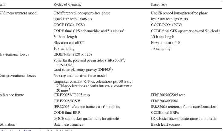
Table 1 Summary of dynamical and measurement models employed for the orbit determination of GOCE

Item Reduced-dynamic Kinematic

GPS measurement model Undifferenced ionosphere-free phase Undifferenced ionosphere-free phase igs05.atxa_{resp. igs08.atx igs05.atx resp. igs08.atx}

GOCE PCOs+PCVs GOCE PCOs+PCVs

CODE final GPS ephemerides and 5 s clocksb CODE final GPS ephemerides and 5 s clocks

30-h arc length 30-h arc length

Elevation cut-off 0◦ Elevation cut-off 0◦

10 s sampling 1 s sampling

Gravitational forces EIGEN-5Sc_{(120× 120)}

Solid Earth, pole and ocean tides (IERS2003d_, FES2004e₎

Luni-solar-planetary gravity (DE405f) Non-gravitational forces No drag and radiation force model

Empirical constant RTN-accelerations per 30 h arc; RTN-accelerations at 6 min intervals, constraints: 20 nm/s2

Reference frame ITRF2005g_{/IGS05 resp. ITRF2005/IGS05 resp.}

ITRF2008/IGS08 ITRF2008/IGS08

IERS2003 reference frame transformations IERS2003 reference frame transformations

CODE final ERPs CODE final ERPs

GOCE star tracker quaternions for attitude GOCE star tracker quaternions for attitude

Estimation Batch least squares Batch least squares

a_{Schmid et al.(2007), used until April 16, 2011} b_{Bock et al.(2009)}

c_{Förste et al.(2008)} d_{McCarthy and Petit(2004)} e_{Lyard et al.(2006)} f_{Standish(1998)} g_{Altamimi et al.(2007),} used until April 16, 2011

checks (orbit overlaps and consistency) were performed to guarantee quality and consistency.

2.1 Operational processing

2.1.1 Orbit overlaps

The processing batches of 30 h allow it to study the overlaps between two consecutive arcs. In order to avoid boundary effects only 5 h overlap periods (21:30–02:30) are checked. Figure 1 shows the RMS values of the overlaps for the reduced-dynamic orbits in radial, along-track, out-of-plane directions, as well as the 3D overlaps for the entire mis-sion until October 20, 2013. The large data gap in summer of 2010 was caused by a problem in the satellite telemetry caus-ing data loss for about 2 months (Floberghagen et al. 2011). Except for very few days, the overlaps are very consistent at a level of 1 cm in 3D. At the very beginning of the mission in April 2009, the attitude data were incomplete or not avail-able at all and between 12 and 28 February 2010, a spacecraft anomaly occurred (Floberghagen et al. 2011). These are only

Jul Jan Jul Jan Jul Jan Jul Jan Jul 0 2 4 6 8 RMS (cm) Date in 2009−2013

radial +6cm along−track +4cm out−of−plane +2cm 3−D

Fig. 1 PSO—RMS of 5-h overlaps of the reduced-dynamic orbits for entire mission; values for radial, along-track and out-of-plane directions are shifted +6 cm, +4 cm and +2 cm, respectively

two examples of special events, for most of the other days where the RMS of the overlaps is exceptionally high a respon-sible event may be found in the monthly L1B data reports, as well. The parametrization of the reduced-dynamic orbit was not optimized for these days, and the constraints for the accelerations might be too tight. Therefore, the RMS of the overlaps shows larger values than normal on these days. The parametrization was not adapted for these days. Obviously, this is not ideal for all days, but this strategy is easy to realize and it is traceable in an operational environment.

Jul Jan Jul Jan Jul Jan Jul Jan Jul −4 −2 0 2 4 Mean (cm) Date in 2009−2013 radial +2cm along−track out−of−plane −2cm

Fig. 2 PSO—mean offsets of 5-h overlaps of the reduced-dynamic orbits for entire mission; mean offsets in radial and out-of-plane direc-tion are shifted +2 cm and−2 cm, respectively

74 74.5 75 75.5 76 76.5 77 77.5 78 −10 −5 0 5 10 −7 m/s 2 74.85 74.9 74.95 75 75.05 75.1 75.15 −5 0 5 Day of Year 2012 10 −7 m/s 2

Fig. 3 Top estimated empirical accelerations in out-of-plane direction for days 074–077 (14–17 March) in 2012; bottom zoom into overlap interval from day 074 and 075 (14 and 15 March), 2012

Inspecting the corresponding mean values of the overlaps in Fig.2, one can notice that in general the out-of-plane com-ponent shows larger variations and has a larger noise than the two other components. This is because the out-of-plane com-ponent is very sensitive to systematic errors in POD (Jäggi et al. 2009).

In addition, one may notice that often the mean val-ues of the out-of-plane direction are significantly larger and of opposite sign for consecutive days. This happened on days when the gradiometer calibration took place.5For this purpose, the satellite was shaken (Frommknecht et al. 2011). The shaking periods lasted for about 24 h, e.g., from 10:37:37 UTC on 15 March 2012 to 09:03:32 UTC on 16 March 2012. As the calibration started in the middle of the day, three consecutive days are affected in the overlap statistics. Figure 3 shows the estimated empirical (6-min piece-wise constant) accelerations plus the estimated con-stant acceleration in out-of-plane direction for four consec-utive days centered around the gradiometer calibration on 15–16 March, 2012 (days 075–076, 2012). The duration of the calibration is marked by the two black vertical lines in the

5_{http://earth.eo.esa.int/missions/goce/monthly/.}

top panel. The estimated accelerations are noticeably larger during the calibration period, due to the additional acceler-ations caused by the shakings. The bottom figure presents a zoom into the overlap interval from 14 and 15 March, 2012 (days 074 and 075). There is a constant offset between the accelerations of days 074 and 075 of about 3×10−8 m_s2. Using

the relationship (Meindl et al. 2013)

δw = W

n2 (1)

with the mean motion n of the satellite and the acceleration

W = 3 × 10−8 m_s2 in out-of-plane direction, we obtain an

off-setδw of approx. 2.2 cm. This value corresponds to the mean offset of−2.24 cm in the overlaps for the reduced-dynamic orbits of days 074 and 075, 2012 and to the equivalent offset with opposite sign of +2.00 cm for the accelerations between days 076 and 077, 2012. The constant acceleration differ-ence in the out-of-plane direction leads to a constant offset between the reduced-dynamic orbits of the consecutive days. The constant difference in the out-of-plane accelerations is caused by a too tight constraining for the piece-wise constant accelerations, which does not allow to compensate the much larger accelerations in the out-of-plane direction caused by the satellite shaking.

2.1.2 Orbit consistency

The differences between the reduced-dynamic and the kine-matic orbits provide another internal quality measure. These differences give no direct information about the orbit accu-racy, but they are indicators for data quality, because kine-matic orbits are very sensitive to data quality. Figure4shows the arc-wise RMS of these differences in the radial, along-track, and out-of-plane directions, as well as the 3D values for the entire mission. The differences used for the statistics are computed every 10 s only, because the reduced-dynamic orbit is sampled to this interval. In order not to deteriorate the daily values by single outliers in the kinematic orbits, differences larger than 1 m (<0.5%) were removed from the statistics.

Jul Jan Jul Jan Jul Jan Jul Jan Jul 0 3 6 9 12 15 18 RMS (cm) Date in 2009−2013

radial +9cm along−track +6cm out−of−plane +3cm 3−D

Fig. 4 PSO—comparison between reduced-dynamic and kinematic orbits; RMS of the orbit differences; values for radial, along-track and out-of-plane directions are shifted +9 cm, +6 cm and +3 cm, respectively

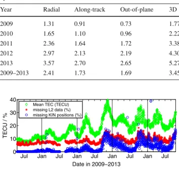
The RMS of the differences in essence shows the same signature in all components. The days with large values in the overlaps show also larger RMS values in the differ-ences between the reduced-dynamic and kinematic orbits. The RMS of the differences is, however, not at the same level for the entire time interval. Starting with September 2010, the differences got slightly larger and in the periods of March/April 2011, October 2011–April 2012, and from Sep-tember 2012 until the end of the mission the RMS of the dif-ferences is significantly larger in all components. The mean values listed in Table2confirm in numbers the increase in the RMS values. Figure5shows similar signatures as in the orbit differences for the mean total electron content (TEC), esti-mated by the Center for Orbit Determination in Europe (Dach et al. 2009, CODE), reflecting the solar activity, as well as for the percentage of missing data on the second GPS frequency (L2) and of missing kinematic positions in the PSO. The correlation between these three quantities and the increased RMS of the differences between reduced-dynamic and kine-matic orbits (Fig.4) are obvious. Even seasonal variations, e.g., the minima around July and maxima around Novem-ber, are at the same places in all displayed quantities. The correlation between the mean TEC and the 3D RMS values in Fig.4is 0.70, between mean TEC and missing L2 data 0.86 and between mean TEC and missing kinematic posi-tions 0.74.

The impact of missing L2 observations on the GPS data availability was already reported by van den IJssel et al. (2011). Observations are mainly missing in the polar regions

Table 2 Mean RMS (cm) values from differences between reduced-dynamic and kinematic orbits

Year Radial Along-track Out-of-plane 3D

2009 1.31 0.91 0.73 1.77 2010 1.65 1.10 0.96 2.22 2011 2.36 1.64 1.72 3.38 2012 2.97 2.13 2.19 4.30 2013 3.57 2.70 2.65 5.27 2009–2013 2.41 1.73 1.69 3.45

Jul Jan Jul Jan Jul Jan Jul Jan Jul 0 10 20 30 40 Date in 2009−2013 TECU / %

Mean TEC (TECU) missing L2 data (%) missing KIN positions (%)

Fig. 5 Mean TEC (TECU) values and corresponding percentage of missing L2 data and missing kinematic positions in the PSO

near the geomagnetic poles and around the geomagnetic equator. The increasing solar activity visibly documented by the mean TEC values had obviously a negative influence on the tracking performance of the SSTI—and the situation got worse with the years. Additionally, the ascending node of the GOCE orbit was not fixed, but was slowly moving from ini-tially 18:00 local time towards midnight. By the beginning of April 2013, the local time of the ascending node was, there-fore, at about 19:20 (M. Fehringer, ESA, private communi-cation). The ascending arcs of the satellite, therefore, passed more and more through an environment of large ionospheric scintillations shortly after dusk (Basu and Groves 2001). This led to increasing tracking problems around the geomagnetic equator for ascending passes.

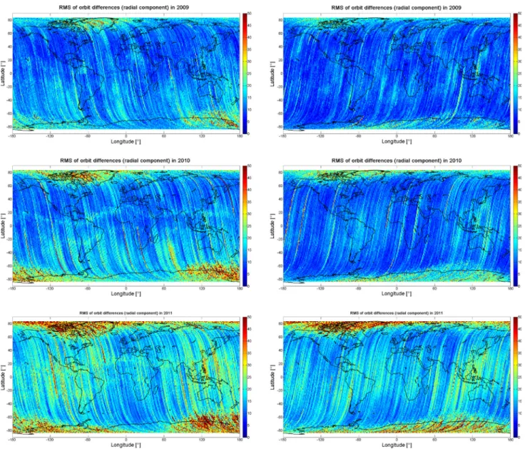
Figure6shows the radial RMS of the differences between reduced-dynamic and kinematic orbits in a geographical dis-tribution for the years 2009 to 2011 separate for ascend-ing (left column) and descendascend-ing (right column) passes. The RMS values are largest around the geomagnetic poles (Northern Canada/Greenland and south of Australia) and the affected area gets larger year after year. The values them-selves also increase from year to year. This development is the main reason for the increasing RMS values in Fig.4. Other systematics around the geomagnetic equator are visible in these figures, which do, however, not cause the increasing RMS values. These systematics are not very large, but unfor-tunately they prominently map into the GPS-only gravity field solutions derived from the kinematic positions (Baur et al. 2014). More investigations on these systematics are provided inJäggi et al.(2014).

In summary, the internal validation of the GOCE PSO product shows that the orbit determination could be run with the same settings for the entire mission irrespective of whether the satellite was in drag-free mode or not. The orbit parametrization for the reduced-dynamic orbit was not ideal for some short time periods in non-drag-free mode, but it was still possible to derive orbit solutions of good quality for these days as well. The kinematic orbit is not sensitive whether the drag-free mode is on or off, and therefore the quality is not directly affected by the flight mode. It is, however, sensitive to data problems and to data gaps and therefore the qual-ity measure derived from comparing reduced-dynamic and kinematic orbits is sensitive to data problems.

2.2 Improvements in external validation

Whether the orbit accuracy is significantly affected by the data problems mentioned in the previous section can only be assessed by independent measurements. The SLR measure-ments to GOCE may serve as such external validations for the GOCE orbits derived from GPS data. In order to support the SLR tracking of GOCE by the International Laser Rang-ing Service (Pearlman et al. 2002, ILRS), additional orbit

Fig. 6 RMS (mm) of radial differences between reduced-dynamic and kinematic PSO in a geographical distribution separated in ascending and descending passes for 2009, 2010, and 2011

predictions were made available from AIUB based on GPS-derived orbits (Jäggi et al. 2011). The models as listed in the GOCE Standards document (European 2010) were used for the validation of the GOCE orbits with SLR measurements. Nadir-dependent range corrections for the laser retro-reflector array on GOCE were made available by ESA (Bigazzi and Frommknecht 2010) at the beginning of the mission. The studies byBock et al.(2011a,b) used this infor-mation for SLR validation. In the meantime,Montenbruck and Neubert(2011) provided several models of azimuth– nadir dependent range corrections for the GOCE and CryoSat (SP 2003) laser retro-reflector arrays. The retro-reflector array on GOCE consisted of seven corner cubes. Six cubes were mounted symmetrically around one center cube, and the range correction was then computed depending on the

nadir and the azimuth angle of the incoming laser pulse. The corresponding correction map for the nearest-prism approx-imation [details may be found inMontenbruck and Neubert (2011)], which was selected for the GOCE SLR validation, is shown in Fig.7.

In addition to the correction map, the tilting angle of 5◦ of the retro-reflector array with respect to the satellite body (Bigazzi and Frommknecht 2010) was considered for the validation. In order to check the impact of these two improvements in the external validation of the GOCE orbits, they were applied for the time interval from day 251/2010 to 226/2011 (September 8, 2010–August 14, 2011) in two different test cases parallel to the original settings (nadir-dependent + no tilt). The resulting statistics of the validation are contained in Table 3. The standard deviation dropped

down from 1.82 to 1.45 cm when applying the tilt of the reflector array. Furthermore, the mean offset got close to zero when additionally applying the range corrections from the improved modeling of the laser retro-reflector array with the nearest-prism approximation. The example shows that small modeling deficiencies in the SLR observable may already be seen in the validation results.

0 90 60 30 −30 −25 −20 −15

Fig. 7 GOCE azimuth–nadir dependent range corrections (mm) for the laser retro-reflector array (Montenbruck and Neubert 2011, nearest-prism approximation,). Azimuth of 0◦nominally points into flight direc-tion

Table 3 SLR validation of reduced-dynamic orbits from day 251/2010–226/2011

Range corrections + tilt Mean (cm) Standard deviation (cm) Nadir-dependent + no tilt 0.55 1.82 Nadir-dependent + 5◦tilt 0.52 1.45 Nearest-prism approximation + 5◦tilt 0.01 1.44

The SLR residuals for the entire mission are shown in Fig.8for the reduced-dynamic orbits and in Fig.9for the kinematic orbits. The corresponding statistics are listed in Table 4. In order not to deteriorate the validation by sin-gle outliers, SLR residuals larger than 20 cm (<0.3%) were excluded. The results for the kinematic orbits are worse than for the reduced-dynamic orbits. This is not surprising, because kinematic orbits are more sensitive to data problems. The yearly values show a degradation of the orbit quality toward the end of the mission. The orbit accuracy suffers from the mentioned data problems and gaps mainly for the kinematic orbits.

The overall RMS value for the reduced-dynamic orbit is 1.84 cm, which is still better than the required 2-cm orbit accuracy. The overall accuracy of the kinematic orbits with 2.42 cm is slightly larger than 2 cm.

3 Beyond HPF: orbit determination using accelerometer data

The six accelerometers on GOCE form the gradiometer. Dif-ferential and common-mode accelerations can be derived from their readings. Differential accelerations are used for the gravity field determination. The common-mode accelera-tions provide a measure of the non-gravitational forces acting on the satellite and they served as input for the DFAC system. The official reduced-dynamic PSO solution did not make use of the common-mode accelerations, because one wanted to be independent from the availability of the common-mode accelerations for the official operational orbit solutions. The question is, however, whether one may get equivalent or even better results by using them in the reduced-dynamic orbit determination process.

Fig. 8 SLR validation for reduced-dynamic orbits of PSO; mean offset 0.18 cm, RMS 1.84 cm

APR JUL OCT JAN APR JUL OCT JAN APR JUL OCT JAN APR JUL OCT JAN APR JUL OCT −200 −150 −100 −50 0 50 100 150 200 SLR Residuals [mm] Date in 2009 − 2013

SLR Residuals for GOCE (RD PSO orbit)

Yarragadee Greenbelt Monument Peak Haleakala Tahiti Koganei Concepcion Hartebeesthoek Zimmerwald San Fernando Mt. Stromlo Graz Herstmonceux Potsdam Grasse Matera Wettzell

Fig. 9 SLR validation for kinematic orbits of PSO; mean offset 0.10 cm, RMS 2.42 cm

APR JUL OCT JAN APR JUL OCT JAN APR JUL OCT JAN APR JUL OCT JAN APR JUL OCT −200 −150 −100 −50 0 50 100 150 200 SLR Residuals [mm] Date in 2009 − 2013

SLR Residuals for GOCE (KIN PSO orbit)

Yarragadee Greenbelt Monument Peak Haleakala Tahiti Koganei Concepcion Hartebeesthoek Zimmerwald San Fernando Mt. Stromlo Graz Herstmonceux Potsdam Grasse Matera Wettzell

Table 4 SLR validation for both orbit types; mean(cm)±RMS(cm)

Year Red.-dynamic Kinematic

2009 0.24± 1.73 0.29± 1.91 2010 −0.10 ± 1.56 −0.12 ± 1.84 2011 0.20± 1.53 0.12± 2.36 2012 0.10± 1.94 −0.05 ± 2.78 2013 0.63± 2.62 0.45± 3.17 2009–2013 0.18± 1.84 0.10± 2.42

3.1 Characteristics of the accelerometer data

The GOCE accelerometer data refer to the gradiometer refer-ence frame, which is a right-handed system with X pointing approximately into flight direction, Y is orthogonal to X and is parallel to the instantaneous direction of the orbital angu-lar momentum, and Z points approximately in nadir direction (European 2010). It would be best to study the accelerome-ter data in this original XYZ system. For practical reasons, we rotate them into the RAO system, where R points into the radial direction, A is orthogonal to R within the orbital plane and approximately points into the along-track direc-tion, and O completes the right-handed system with the out-of-plane component. This transformation gives us the possi-bility to directly compare the accelerometer data with the empirical accelerations estimated in the reduced-dynamic orbit determination for the PSO (which are estimated in the RAO system). Accelerometer data are biased observations. Before rotating the data into the RAO system, a mean offset is subtracted for all three directions, respectively. In the orbit determination process, three constant offsets in the directions of the RAO system are estimated and absorb the remain-ing offsets in the accelerometer data. Scale parameters are

not estimated, because they are very stable and close to one (Bouman et al. 2011).

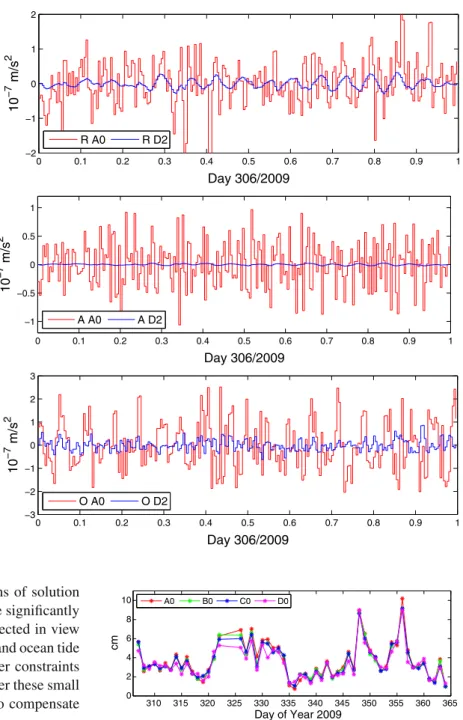
Figure 10 compares the measured accelerometer data

rotated into the RAO-system with the estimated piece-wise constant accelerations from the reduced-dynamic orbit deter-mination for day 306 of the year 2009 (November 2, 2009). In R, only a small correlation (0.14) between the accelerom-eter data (red) and the estimated 6-min piece-wise constant accelerations (blue) may be noticed. The comparison in A shows no correlation at all (−0.01). In O, the correlation is pronounced (0.60). The estimated accelerations closely fol-low the measured accelerometer data.

Our first goal was to find physically more meaningful constraints for the empirical accelerations when not using the accelerometer data for the orbit determination. The offi-cial reduced-dynamic PSO is computed with the same con-straint for all empirical accelerations in all three directions (σ = 2.0 × 10−8 m_s2, σ0 = 0.001 m of phase

observa-tions). This value was derived empirically at the beginning of the mission. If we look at the different variations in the accelerometer measurements, more realistic values for the constraints may be certainly derived from the accelerometer data themselves (assuming that the neglection of accelerom-eter data represents the largest source of mismodelings).

Since we used 6-min piece-wise constant empirical accel-erations, we took the mean values over 6 min of the accelerometer measurements and computed the RMS of these mean values over 24 h. We found that the daily RMS values are almost constant over periods of several months (valid for the test period used in Sect.3.2), and therefore one may translate these RMS values to constant constraints for the corresponding directions.

If we use the accelerometer data in the orbit determina-tion process in a further step to model the sum of all non-gravitational accelerations, they should replace the

empiri-Fig. 10 Comparison between accelerometer data and 6-min piece-wise constant

accelerations from the reduced-dynamic orbit determination; day 306/2009; top: R; 0.14 correlation coefficient, middle: A;−0.01, bottom: O; 0.60 0 0.1 0.2 0.3 0.4 0.5 0.6 0.7 0.8 0.9 1 −2 −1 0 1 2 Day 306/2009 10 −7 m/s 2 R acc R est 0 0.1 0.2 0.3 0.4 0.5 0.6 0.7 0.8 0.9 1 −1 −0.5 0 0.5 1 Day 306/2009 10 −7 m/s 2 A acc A est 0 0.1 0.2 0.3 0.4 0.5 0.6 0.7 0.8 0.9 1 −3 −2 −1 0 1 2 3 Day 306/2009 10 −7 m/s 2 O acc O est

cally estimated accelerations to a large extent. It should thus be possible to tighten the constraints significantly, because only small unmodeled signals should remain to be compen-sated by the empirical parameters. For this scenario, we use 10 % of the constraint derived from the accelerometer data. This value is empirical in nature.

3.2 Test scenario

Different reduced-dynamic orbits with and without using accelerometer data and with different constraints were com-puted for the time interval from November 2 to December 30, 2009 (306–364/2009). In order to study the impact of the background models, different gravity field and ocean tide models up to different truncation are used as well. As ref-erence solution, we used the official reduced-dynamic PSO solution (central 24 h). A detailed description of the models and parameters used may be found in Table1.

The models relevant for this study are given in Table5. The left column lists the different gravity field and ocean tide models used with different truncations for solution types A, B, C and D. Solution type A is computed without

common-mode accelerometer data. Solution types B, C and D are using them in the orbit determination process. The corre-sponding constraints are listed in the very first row. Solu-tion type 0 uses the same constraint as the official reduced-dynamic PSO solution for all three directions. Solution type 1 applies a tighter, but equal constraint for all three direc-tions, and solution type 2 uses different constraints for the three directions, which were derived from the accelerometer data.

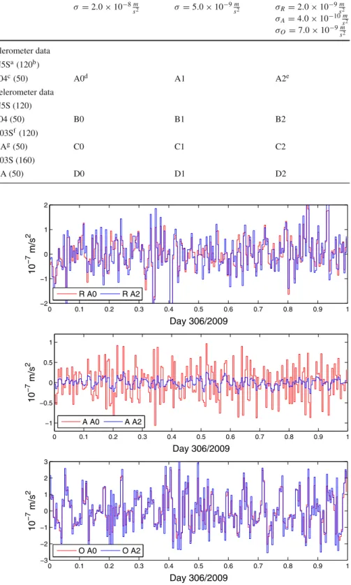
Figure11shows the estimated accelerations of solution A0 and A2. The only difference between the two solutions is the constraints for the estimated accelerations. The constraints for solution A2 were derived from the measured accelerations and should, therefore, be more realistic than the common con-straints used for solution A0. The values listed in the top right of Table5were already reduced to 10 % of the values derived from the measured accelerations. For solution A2, these val-ues are thus multiplied again by a factor of 10, because we do not use the accelerometer data for the orbit determination and the full signal has to be absorbed by the estimated accelera-tions. In radial direction R, where the constraint for solution A2 is still the same as for solution A0, the accelerations are,

Table 5 Summary of

reduced-dynamic orbit solutions

a_{Förste et al.(2008)} b_{Used up to degree and order} c_{Lyard et al.(2006)} d_{Corresponds to official} reduced-dynamic PSO solution e_{Constraints are multiplied by} factor 10

f_{Mayer-Gürr et al.(2012)} g_{Savcenko and Bosch(2008)}

σ = 2.0 × 10−8 m

s2 σ = 5.0 × 10−9 m_s2 σR= 2.0 × 10−9 m_s2

σA= 4.0 × 10−10 m_s2

σO= 7.0 × 10−9 m_s2

w/o accelerometer data

EIGEN5Sa₍₁₂₀b₎

FES2004c_{(50) A0}d _{A1 A2}e

With accelerometer data EIGEN5S (120) FES2004 (50) B0 B1 B2 GOCO03Sf(120) EOT08Ag(50) C0 C1 C2 GOCO03S (160) EOT08A (50) D0 D1 D2 Fig. 11 Comparison of estimated accelerations for solution A0 and A2; day 306/2009; top: R, middle: A, bottom: O 0 0.1 0.2 0.3 0.4 0.5 0.6 0.7 0.8 0.9 1 −2 −1 0 1 2 Day 306/2009 10 −7 m/s 2 R A0 R A2 0 0.1 0.2 0.3 0.4 0.5 0.6 0.7 0.8 0.9 1 −1 −0.5 0 0.5 1 Day 306/2009 10 −7 m/s 2 A A0 A A2 0 0.1 0.2 0.3 0.4 0.5 0.6 0.7 0.8 0.9 1 −3 −2 −1 0 1 2 3 Day 306/2009 10 −7 m/s 2 O A0 O A2

however, slightly different. The correlation to the measured accelerations is 0.24, and thus larger than for solution A0. The estimated accelerations in along-track direction A are significantly smaller due to the tighter constraint (correlation to measured accelerations 0.04). Due to the high degree of correlation between the radial and along-track components,

the accelerations in R have obviously absorbed some unmod-eled signal. The accelerations in out-of-plane direction O for solution A2 (correlation to measured accelerations 0.51) are slightly larger than for solution A0, which can be explained by the weaker constraint for the O component for A2 than for A0.

Fig. 12 Comparison of estimated accelerations for solution A0 and D2; day 306/2009; top: R, middle: A, bottom: O 0 0.1 0.2 0.3 0.4 0.5 0.6 0.7 0.8 0.9 1 −2 −1 0 1 2 Day 306/2009 10 −7 m/s 2 R A0 R D2 0 0.1 0.2 0.3 0.4 0.5 0.6 0.7 0.8 0.9 1 −1 −0.5 0 0.5 1 Day 306/2009 10 −7 m/s 2 A A0 A D2 0 0.1 0.2 0.3 0.4 0.5 0.6 0.7 0.8 0.9 1 −3 −2 −1 0 1 2 3 Day 306/2009 10 −7 m/s 2 O A0 O D2

Figure12shows the estimated accelerations of solution D2 in comparison to A0. The accelerations are significantly smaller in all three components, which is expected in view of the improved modeling (better gravity field and ocean tide model, higher truncation) and the much tighter constraints for D2 compared to A0. The question is whether these small constraints of solution D2 are large enough to compensate for remaining model deficiencies.

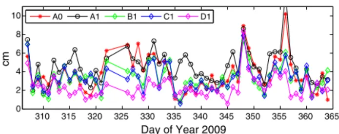
The comparisons between the estimated accelerations are, however, not helpful to resolve this question. The quality of the resulting orbits has to be assessed in a different way. Therefore, we inspect the 3D orbit difference between sub-sequent orbital arcs at midnight. The test solutions are only computed in 24-h batches not allowing for long overlaps. A small orbit difference at midnight means that the sub-sequent orbits are consistent. The orbit difference at mid-night is, therefore, a quality indicator for the solution type. Figure 13 shows these orbit differences for the solution types 0 using the constraints of the reduced-dynamic ref-erence solution. All four solutions A0–D0 are on the same level and no significant differences may be recognized. This might be surprising at first sight, because solutions B0–

310 315 320 325 330 335 340 345 350 355 360 365 0 2 4 6 8 10 Day of Year 2009 cm A0 B0 C0 D0

Fig. 13 Orbit differences at midnight for solution types 0

D0 are using the measured accelerometer data in the orbit determination process. In these cases, the constraints are not tight enough and the degree of freedom is too high to ben-efit from the accelerometer data in the orbit determination process.

Figure14shows the orbit differences for solution types A1–D1 together with reference solution A0. The tighter con-straints for all components result in a different signature for the orbit differences. Solution A1 is in general worse and Solution D1 in general better than solution A0, but for the other two solutions B1 and C1 the result is not that clear.

310 315 320 325 330 335 340 345 350 355 360 365 0 2 4 6 8 10 Day of Year 2009 cm A0 A1 B1 C1 D1

Fig. 14 Orbit differences at midnight for solution types A1–D1 and A0 310 315 320 325 330 335 340 345 350 355 360 365 0 2 4 6 8 10 Day of Year 2009 cm A0 A2 B2 C2 D2

Fig. 15 Orbit differences at midnight for solution types A2–D2 and A0

Table 6 SLR validation for different solution types; mean (cm)± RMS (cm) 0 1 2 A 0.35± 2.01 0.31± 2.14 0.31± 1.90 B 0.32± 1.99 0.23± 2.01 0.17± 2.02 C 0.33± 1.99 0.22± 1.98 0.18± 1.96 D 0.34± 1.98 0.28± 1.89 0.22± 1.79

Looking eventually at the orbit differences for solutions of type 2 in Fig.15three issues may be noticed. First, solu-tion A2, which does not use accelerometer data but more realistic constraints than solution A0 has smaller orbit differ-ences than the reference solution A0. Second, solutions B2 and C2 do not show a common improvement compared to solution A0 and third, solution D2 has clearly the smallest orbit differences of all solution types.

The SLR validation for the different solution types is listed in Table6, which confirms the results of the orbit difference analysis. The validation for solutions A0–D0 is on a similar level for all four solutions, only a slight improvement may be noticed from A0 toward D0. The solutions B1–D1 have a smaller offset (mean), but except for solution D1 they also are on a similar level as the reference solution A0. Solution A2 has a better SLR validation than solution A0. Solutions B2 and C2 have the smallest offest, but the RMS is not yet showing any major improvement. Solution D2, however, is definitely the best solution as viewed by SLR.

From these test series we conclude that, on the one hand, the use of more realistic constraints for the estimated accel-erations improves the orbit quality. On the other hand, the

simple use of accelerometer data with the same models and parametrization as used for the solutions without accelerom-eter data does not significantly improve the orbit quality. The combination, however, of realistic constraints and better background models as it is applied for solution D2 is the best choice and improves the orbit quality significantly. The main difference for solution D2 is that it uses a higher truncation (160 instead of 120) of the gravity field model than for solu-tion types A–C. This result shows also that the unmodeled or not sufficiently well-modeled gravitational forces are still dominant due to the very low orbital altitude. They cannot be absorbed well enough by the estimated 6-min piece-wise constant accelerations.

4 Summary

The official GOCE PSO product has been generated very consistently for the entire mission. The reduced-dynamic orbits show for single days only larger values in the overlap statistics. In most cases, larger values occur on days where the satellite was not flying in drag-free mode. The days of the gradiometer calibrations “pop up” in the overlaps of the reduced-dynamic orbits. The satellite shakings cause an addi-tional acceleration, which cannot be fully absorbed by the estimated accelerations in out-of-plane direction using the adopted constraints. This circumstance leads to larger mean offsets in this direction.

The quality of the kinematic orbits slightly decreased towards the end of the mission due to the increased solar activity leading to more tracking problems on the GPS L2 fre-quency, and thus an increased number of data gaps. The orbit consistency checks in terms of orbit differences between the reduced-dynamic and kinematic orbits revealed this effect. The yearly SLR validation also confirms that the kinematic orbits are more affected by tracking problems and data gaps than the reduced-dynamic orbit. The SLR RMS values are increasing towards the end of the mission, more significantly for the kinematic orbits. The overall SLR validation, how-ever, still indicates an outstanding 1D accuracy of 1.84 cm for the reduced-dynamic and 2.42 cm for the kinematic orbits for the entire mission.

Modeling the range corrections of the laser retro-reflector array with a nearest-prism approximation has significantly improved the SLR validation. Introducing the tilt of the reflector array with respect to the satellite body also improved the SLR validation.

A study showed that more realistic constraints derived from the accelerometer data may improve the reduced-dynamic orbit results significantly. If one uses the accelerom-eter data directly in the reduced-dynamic orbit daccelerom-etermination procedure and additionally makes use of better background models (mainly using higher truncation than 120 for the

grav-ity field model) than for the official reduced-dynamic PSO product, the orbit accuracy can be improved even more. Our findings should be considered for a possible reprocessing of the PSO.

Acknowledgments This work was partly performed in the frame of the GOCE High-level Processing Facility (HPF), which is funded by ESA. The support of ESA is gratefully acknowledged. The activities of the CODE analysis center of the IGS provide the basis for our work. CODE is a joint venture of AIUB, Swiss Federal Office of Topogra-phy (swisstopo), Wabern, Switzerland, the German Federal Office of Cartography and Geodesy (BKG), Frankfurt a. Main, Germany, and the Institut für Astronomische and Physikalische Geodäsie (IAPG), Tech-nische Universität München, Germany.

References

Altamimi Z, Collilieux X, Legrand J, Garayt B, Boucher C (2007) ITRF2005: a new release of the international terrestrial reference frame based on time series of station positions and earth orien-tation parameters. J Geophs Res 112(B9):401–419. doi:10.1029/ 2007JB004949

Andreis D, Canuto E (2005) Drag-free and attitude control for the GOCE satellite. In: 44th IEEE conference on decision and control, 2005 and 2005 European control conference CDC-ECC05, pp 4041–4046. doi:10.1109/CDC.2005.1582794

Basu S, Groves KM (2001) Specification and forecasting of outages on satellite communication and navigation systems. In: Song P, Singer HJ, Siscoe GL (eds) Space weather geophysical monograph series, vol 125, pp 424–430. doi:10.1029/GM125p0423

Baur O, Bock H, Höck E, Jäggi A, Krauss S, Mayer-Gürr T, Reubelt T, Siemes C, Zehentner N (2014) Comparison of GOCE-GPS gravity fields derived by different approaches. J Geod. doi: 10.1007/s00190-014-0736-6

Bigazzi A, Frommknecht B (2010) Note on GOCE instruments position-ing, Issue 3.1. http://earth.esa.int/download/goce/GOCE-LRR-GPS-positioning-Memo_3.1_[XGCE-GSEG-EOPG-TN-09-0007v3.1] Bock H, Jäggi A, Švehla D, Beutler G, Hugentobler U, Visser P (2007)

Precise orbit determination for the GOCE satellite using GPS. Adv Space Res 39(10):1638–1647. doi:10.1016/j.asr.2007.02.053

Bock H, Dach R, Jäggi A, Beutler G (2009) High-rate GPS clock correc-tions from CODE: support of 1 Hz applicacorrec-tions. J Geod 83(11):1083– 1094. doi:10.1007/s00190-009-0326-1

Bock H, Jäggi A, Meyer U, Dach R, Beutler G (2011) Impact of GPS antenna phase center variations on precise orbits of the GOCE satel-lite. Adv Space Res 47(11):1885–1893. doi:10.1016/j.asr.2011.01. 017

Bock H, Jäggi A, Meyer U, Visser P, van den IJssel J, van Helleputte T, Heinze M, Hugentobler U, (2011b) GPS-derived orbits for the GOCE satellite. J Geod 85(11):807–818. doi: 10.1007/s00190-011-0484-9

Bouman J, Fiorot S, Fuchs M, Gruber T, Schrama E, Tscherning C, Veicherts M, Visser P (2011) GOCE gravitational gradients along the orbit. J Geod 85(11):791–805. doi:10.1007/s00190-011-0464-0

Bouman J, Floberghagen R, Rummel R (2013) More than 50 years of progress in satellite gravimetry. EOS Trans Am Geophys Union 94(31):269–274. doi:10.1002/2013EO31

Dach R, Brockmann E, Schaer S, Beutler G, Meindl M, Prange L, Bock H, Jäggi A, Ostini L (2009) GNSS processing at CODE: status report. J Geod 83(3–4):353–365. doi:10.1007/s00190-008-0281-2

Dach R, Beutler G, Bock H, Fridez P, Gäde A, Hugentobler U, Jäggi A, Meindl M, Mervart L, Prange L, Schaer S, Springer T, Urschl C, Walser P (2007) Bernese GPS Software Version 5.0. Astronomical

Institute, University of Bern, Bern, Switzerland.http://www.bernese. unibe.ch/docs/DOCU50, user manual

European GOCE Gravity Consortium (EGG-C) (2010) GOCE Stan-dards, GO-TN-HPF-GS-0111. http://earth.esa.int/pub/ESA_DOC/ GOCE/GOCE_Standards_3.2

Floberghagen R, Fehringer M, Lamarre D, Muzi D, Frommknecht B, Staiger C, Piñeiro J, da Costa A (2011) Mission design, operation and exploitation of the Gravity field and steady-state Ocean Circulation Explorer (GOCE) mission. J Geod 85(11):749–758. doi:10.1007/ s00190-011-0498-3

Förste C, Flechtner F, Schmidt R, Stubenvoll R, Rothacher M, Kusche J, Neumayer H, Biancale R, Lemoine JM, Barthelmes F, Bruinsma S, König R, Meyer U (2008) EIGEN-GL05C—a new global com-bined high-resolution GRACE-based gravity field model of the GFZ-GRGS cooperation. Geophys Res Abstr 10, EGU2008-A-03426 Frommknecht B, Lamarre D, Meloni M, Bigazzi A, Floberghagen R

(2011) GOCE level1b data processing. J Geod 85(11):759–775. doi:10.1007/s00190-011-0497-4

van Helleputte T, Doornbos E, Visser P (2009) CHAMP and GRACE accelerometer calibration by GPS-based orbit determination. Adv Space Res 43(12):1890–1896. doi:10.1016/j.asr.2009.02.017

Jäggi A (2007) Pseudo-stochastic orbit modeling of low earth satellites using the global positioning system. Geodätisch-geophysikalische Arbeiten in der Schweiz, Band 73, Schweizerische Geodätische Kommission, Institut für Geodäsie und Photogrammetrie, Eidg. Technische Hochschule Zürich, Zürich

Jäggi A, Hugentobler U, Beutler G (2006) Pseudo-stochastic orbit mod-eling techniques for low-Earth orbiters. J Geod 80(1):47–60. doi:10. 1007/s00190-006-0029-9

Jäggi A, Dach R, Montenbruck O, Hugentobler U, Bock H, Beutler G (2009) Phase center modeling for LEO GPS receiver antennas and its impact on precise orbit determination. J Geod 83(12):1145–1162. doi:10.1007/s00190-009-0333-2

Jäggi A, Bock H, Floberghagen R (2011) GOCE orbit predictions for SLR tracking. GPS Solut 15(2):129–137. doi: 10.1007/s10291-010-0176-6

Jäggi A, Montenbruck O, Moon Y, Wermuth M, König R, Micha-lak G, Bock H, Bodenmann D (2012) Inter-agency comparison of TanDEM-X baseline solutions. Adv Space Res 50(2):260–271. doi:10.1016/j.asr.2012.03.027

Jäggi A, Bock H, Meyer U, Beutler G, van den IJssel J (2014) GOCE -Assessment of GPS-only gravity field estimation. J Geod, in review Jäggi A, Hugentobler U, Bock H, Beutler G (2007) Precise orbit deter-mination for GRACE using undifferenced or doubly differenced GPS data. Adv Space Res 39(10):1612–1619. doi:10.1016/j.asr.2007.03. 012

Kang Z, Tapley B, Bettadpur S, Ries J, Nagel P (2006) Precise orbit determination for GRACE using accelerometer data. Adv Space Res 38(9):2131–2136. doi:10.1016/j.asr.2006.02.021

Koop R, Gruber T, Rummel R (2006) The status of the GOCE high-level processing facility. In: Proceedings of the 3rd GOCE user workshop, 6–8 November 2006, Frascati, Italy, ESA SP-627, pp 199–205 Loiselet M, Stricker N, Menard Y, Luntama JP (2000) GRAS MetOps

GPS-based atmospheric sounder. ESA Bull 102:3844

Lyard F, Lefevre F, Letellier T, Francis O (2006) Modelling the global ocean tides: insights from FES2004. Ocean Dynam 56:394–415. doi:10.1007/s10236-006-0086-x

Mayer-Gürr T, Rieser D, Hoeck E, Brockmann JM, Schuh WD, Kras-butter I, Kusche J, Maier A, Krauss S, Hausleitner W, Baur O, Jäggi A, Meyer U, Prange L, Pail R, Fecher T, Gruber T (2012) The new combined satellite only model GOCO03s. In: International sympo-sium on gravity, geoid and height systems GGHS (2012) Venice. Italy, Presentation

McCarthy DD, Petit G (2004) IERS Conventions 2003. IERS Technical note no.32. Bundesamt für Kartographie und Geodäsie, Frankfurt am Main, Germany

Meindl M, Beutler G, Thaller D, Dach R, Jäggi A (2013) Geocenter coordinates estimated from GNSS data as viewed by perturbation theory. Adv Space Res 51(7):1047–1064. doi:10.1016/j.asr.2012.10. 026

Montenbruck O, Andres Y, Bock H, van Helleputte T, van den IJssel J, Loiselet M, Marquardt C, Silvestrin P, Visser P, Yoon Y, (2008) Tracking and orbit determination performance of the GRAS instru-ment on MetOp-A. GPS Solut 12(4):289–299. doi: 10.1007/s10291-008-0091-2

Montenbruck O, Neubert R (2011) Range correction for the CryoSat and GOCE laser retro-reflector arrays. Technical Note DLR/GSOC 11–01

Pearlman M, Degnan J, Bosworth J (2002) The international laser ranging service. Adv Space Res 30(2):135–143. doi: 10.1016/S0273-1177(02)00277-6

Reigber C, Lühr H, Schwintzer P (2002) CHAMP mission status. Adv Space Res 30(2):129–134. doi:10.1016/S0273-1177(02)00276-4

Rummel R, Yi W, Stummer C (2011) GOCE gravitational gradiometry. J Geod 85(11):777–790. doi:10.1007/s00190-011-0500-0

Savcenko R, Bosch W (2008) EOT08a—empirical ocean tide model from multi-mission satellite altimetry. DGFI Report 81, Deutsches Geodätisches Forschungsinstitut, Munich, Germany

Schmid R, Steigenberger P, Gendt G, Ge M, Rothacher M (2007) Gen-eration of a consistent absolute phase center correction model for GPS receiver and satellite antennas. J Geod 81(12):781–798. doi:10. 1007/s00190-007-0148-y

SP-1272 E (2003) CryoSat science report. ESA Publications Division Standish EM (1998) JPL Planetary and Lunar Ephemerides,

DE405/LE405. JPL IOM 312.F-98-048

Švehla D, Rothacher M (2005) Kinematic precise orbit determination for gravity field determination. In: Sansò F (ed) The proceedings of the international association of geodesy, A Window on the Future of Geodesy, IUGG General Assembly 2003, vol 128, June 30–July 11, 2003, Springer, Sapporo, Japan. pp 181–188. doi 10.1007/3-540-27432-4_32

Tapley B, Bettadpur S, Ries J, Watkins M (2004) GRACE measurements of mass variability in the Earth system. Science 305(5683):503–505 van den IJssel J, Visser P, Doornbos E, Meyer U, Bock H, Jäggi A (2011) GOCE SSTI L2 tracking losses and their impact on POD performance. In: Proceedings of 4th international GOCE user work-shop, 31 March–1 April, 2011, TU München, Munich, Germany, ESA, ESA communications

van Helleputte T (2011) The integration of spaceborne accelerometry in the precise orbit determination of low-flying satellites. PhD thesis, Delft University of Technology

Visser P, van den IJssel J, van Helleputte T, Bock H, Jäggi A, Beutler G, Švehla D, Hugentobler U, Heinze M (2009) Orbit determination for the GOCE satellite. Adv Space Res 43(5):760–768. doi:10.1016/ j.asr.2008.09.016