HAL Id: hal-00133833
https://hal.archives-ouvertes.fr/hal-00133833v2
Submitted on 2 Apr 2007
HAL is a multi-disciplinary open access
archive for the deposit and dissemination of
sci-entific research documents, whether they are
pub-lished or not. The documents may come from
teaching and research institutions in France or
abroad, or from public or private research centers.
L’archive ouverte pluridisciplinaire HAL, est
destinée au dépôt et à la diffusion de documents
scientifiques de niveau recherche, publiés ou non,
émanant des établissements d’enseignement et de
recherche français ou étrangers, des laboratoires
publics ou privés.
Consumer Profile Identification and Allocation
Patrick Letrémy, Marie Cottrell, Eric Esposito, Valérie Laffite, Sally Showk
To cite this version:
Patrick Letrémy, Marie Cottrell, Eric Esposito, Valérie Laffite, Sally Showk. Consumer Profile
Identi-fication and Allocation. Francisco Sandoval, Alberto Prieto, Joan Cabestany, Manuel Grana.
Compu-tational and Ambient Intelligence - 9th International Work-Conference on Artificial Neural Networks,
IWANN 2007, Springer, pp.530-538, 2007, Lecture Notes in Computer Science - 4507,
�10.1007/978-3-540-73007-1�. �hal-00133833v2�
hal-00133833, version 2 - 2 Apr 2007
Consumer Profile Identification and Allocation
Patrick Letr´emy1, Marie Cottrell1,
Eric Esposito2, Val´erie Laffite2and Sally Showk2
1 SAMOS-MATISSE, Universit´e Paris1-Panth´eon-Sorbonne, CES UMR CNRS,
90, rue de Tolbiac, F-75013 Paris, France marie.cottrell, [email protected]
2 Research and Development Division
Gaz de France
eric.esposito, valerie.lafitte, [email protected]
Abstract. We propose an easy-to-use methodology to allocate one of
the groups which have been previously built from a complete learning data base, to new individuals. The learning data base contains continu-ous and categorical variables for each individual. The groups (clusters) are built by using only the continuous variables and described with the help of the categorical ones. For the new individuals, only the categorical variables are available, and it is necessary to define a model which com-putes the probabilities to belong to each of the clusters, by using only the categorical variables. Then this model provides a decision rule to assign the new individuals and gives an efficient tool to decision-makers. This tool is shown to be very efficient for customers allocation in con-sumer clusters for marketing purposes, for example.
Keywords:Kohonen Maps, Profiles, Logistic regression, non-ordered Poly-chotomous Logit Model
1
Introduction
The methodology that we propose in this paper is very general and can be used in many different frames, even if the main applications belong to the marketing domain. A first presentation of the main ideas can be found in [11].
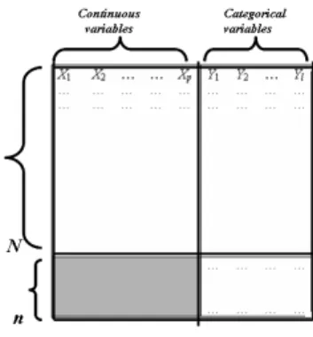
Let us define some general notations: Let X be a database, represented by a N × (p + l)-matrix, where N is the number of individuals, p the number of continuous variables (possibly with missing data) and l the number of categor-ical variables (no missing data are allowed). The first p variables are denoted X1, X2, . . . , Xp, and the other l variables are denoted Y1, Y2, . . . , Yl.
In addition, we have a n × l matrix which corresponds to new individuals. For these new individuals, only the categorical variables Y1, Y2, . . . , Yl are
well-informed and the continuous variables are not available. For example, the N individuals in the database are consumers already registered as customers by a firm and who can be described by their expenses, while the new n individuals have only filled up a form and given some categorical indications (age, housing
Fig. 1.The data
status, education level, etc.) The first step of the study is to define homogeneous groups from the point of view of the continuous variables. The interest of such clustering is double : each cluster corresponds to a typical profile which is a summary of the whole class and the whole group can be treated in the same way by any decision-maker. To follow our example, the direction of sales can use particular targeting techniques to improve the efficiency of the advertising policy towards each cluster.
The second step consists in allocating a cluster to new individuals (for mar-keting purposes, for example). For this goal, it is necessary to define a model which computes the probabilities of belonging to each of the clusters, by using only the categorical variables. The parameters of this model will be estimated from the database X. For this step, the new data can be incomplete and missing values are acceptable.
The paper is organized as follows : Section 2 clarifies the relations between the two types of variables in X and gives indications about the selection of the relevant variables. Section 3 briefly deals with the construction of the clusters and the interpretation of each profile. In Section 4, we present the multinomial logit model to compute the membership probabilities. Then this model can be applied to new individuals in order to assign them to the most probable cluster. Finally section 5 is devoted to a real-world example and applies the proposed methodology to a survey data which contains the consumption structure of Cana-dian consumers, together with some personal categorical variables. Section 6 is a conclusion.
2
Variables selection
As the final goal is to assign an individual described by the categorical variables Y1, Y2, . . . , Yl to a cluster built from the continuous variables X1, X2, . . . , Xp, it
is obvious that the goal cannot be achieved if these two groups of variables are independent!
We assume that all the categorical variables are of interest for the applica-tions since they are the only real characteristics which are available for the new individuals and have to be taken into account by the decision-makers. So it is necessary to select the relevant continuous variables which are strongly related to the categorical ones.
Let us consider the multidimensional l-ways additive ANOVA model ( [14]) where the explained variables are the Xi, when the explanatory variables are
the Indicator Functions of each modality for all the Yj. For each component
i, i = 1, . . . , p, a global Fisher Statistics and a Squared Correlation Coefficient are computed. The variables Xi that give the least significant values are not
considered in what follows.
3
The clustering
First we only take into account the continuous variables X1, X2, . . . , Xpto cluster
the N individuals into K clusters. A that step, any unsupervised classification algorithm can be used. We propose to use a Kohonen algorithm due to several of its properties (see [9], [10], [8], [2], [3], [13]):
– The Kohonen maps are known to produce well-balanced and homogeneous classes,with small quantization error, see [6];
– The visualization of the clusters is easy to interpret, thanks to the self-organization property, since there exists a neighborhood structure between classes;
– The Kohonen algorithm is robust with respect to missing values, since it can be adapted to be used with incomplete data, see [7], [4];
– It is possible to build a Kohonen map having a large number of classes and to reduce this number by using another clustering of the code-vectors and thus get a few clusters which will easily be interpreted and analyzed. These ”macro” clusters are composed of contiguous Kohonen classes, which corrob-orates the self-organization property see [3]. To build this second classifica-tion, several methods are available : one can choose an ascending hierarchical classification or a one-dimensional Kohonen algorithm. The advantage of this latter choice is that the ”macro” clusters are naturally ordered, and this fact facilitates the interpretation and the description.
After the clusters are built and summarized by their code-vector or profile, one can describe them from two points of view :
– The classical statistics (mean, variance, quartile, median) are computed to characterize and distinguish the clusters.
– The repartitions of the modalities for each categorical variable are computed as well as the test values (that is the ratio between the modality percentage inside the cluster and the modality percentage in the global population).
4
The model of allocation
Once the classification stage is achieved, it is necessary to classify new individ-uals, who do not belong to the learning set, in one of the K clusters. A rough method could be to look after the cluster which contains the number of similar individuals. It would be a deterministic allocation method. We prefer a stochastic allocation.
Then, one has to estimate the probability for a new individual to belong to a cluster only from the categorical variables. The chosen model is a non-ordered polychotomous logit model, since the variable to explain (membership probability to a cluster) has more than two values (there are more than two classes!)
Using the non-ordered polychotomous logit model as discriminating tool has been proposed by Schmidt and Strauss, [15]. It is an extension of the binary logit model, which is often used in the studies of appetence or attrition. The explanatory variables are categorical and the variable to explain can take more than two modalities which are not naturally ordered. The model uses the same theoretical frame, since it is estimated by using the maximum likelihood principle, [12], [16]. The CATMOD procedure of SAS software is designed to estimate this kind of model, [1].
One has to choose a class as a reference class, let us suppose that it is the class K. Let us define pk = P (k/y) as the probability that an individual
be-longs to class k, given the fact that it is described by y. Then the non-ordered polychotomous logit model is written as
pk
pK
= exp(y · βk)
for k = 1, 2, . . . , K − 1, where the βk∈Rl are the model parameters.
For each possible y, the CATMOD procedure provides the estimates of pa-rameters βk∈Rp, k = 1, . . . , K−1 and we compute the probabilities p1, p2, . . . , pK
as a function of y and using equation p1+ p2+ . . . + pK= 1.
Then for each new individual m described by ym= (yjm), j = 1, . . . , l and
for each class k, one computes the probability that this individual belongs to class k. The new individual is assigned to the class for which the probability is maximum.
5
Application to Canadian consumers data
We apply the proposed method to a real-world problem: the domestic consump-tion of Canadian families. The data have been provided by Prof. Simon Langlois from the Universit´e of Laval. For 8809 Canadian consumers in 1992, a survey provides the consumption structures, expressed as percentages of the total ex-penditure of the household. Besides, each individual of the survey is also de-scribed by categorical variables (such as Age, Education level, Wealth, and so
on, see below the full list). In a previous publication, ([5]) we have studied the consumptions profiles, but the allocation problem was not dealt with.
The first step is therefore to identify typical profiles and to define clusters in the population, on the sole basis of the consumption structures. Once these profiles and these clusters are defined, the problem consists in allocating a cluster to new consumers (for marketing purposes) by using the categorical variables.
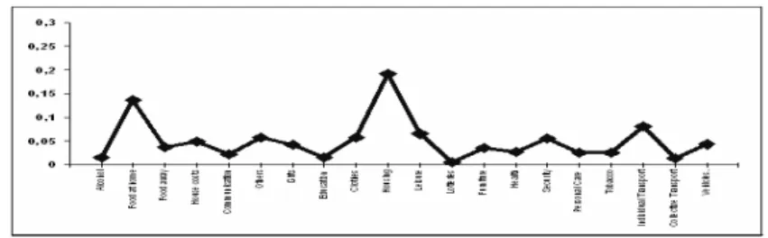
The consumption structure is known through a 19 functions nomenclature: Consumption nomenclature.
Alcohol; Food at home; Food away; House costs; Communication; Financial costs; Gifts; Education; Clothes; Housing expenses; Leisure; Furniture; Health; Security; Personal Care; Tobacco; Individual Transportation; Collective Trans-portation; Vehicles.
See in Fig. 2 the mean consumption structure for the 1992 survey. For each
Fig. 2.Mean Consumption Profile in 1992.
household, the survey provides also 10 categorical variables, which concern the head of the family:
Categorical variables.
For each item, the number between parenthesis indicates the number of modal-ities: Age (4); Language (3); Income (4); Job status (3); Professional category (5); Education level (5); Type of town (3); Region (5); Residency status (5); Wealth index (5).
We follow the successive steps as described above. First, we write down the multivariate l-ways additive ANOVA model. For 5 consumptions variables (Alco-hol; Financial costs; Furniture; Personal Care; Vehicles), the Squared Correlation Coefficients are less than 8% and we decide to skip these variables. So, in the following, we consider that p = 14 and the percentages are computed again with only these 14 consumptions functions.
6
The classification
We separate the 8809 households into two sets: a learning set with 8400 house-holds, and a test set with 409 households. The consumers of this test set will further be assigned to one of the cluster, by using only the categorical variables, and we will compute the number of correct classifications as a performance mea-sure.
We build a 5-cluster classification in two different ways:
– First we consider a Kohonen algorithm using a one-dimensional string and 20 units,the number of which is then reduced to 5 macro-classes, by using another one-dimensional Kohonen algorithm with 5 units, that operates over the 20 code-vectors: Classification C1.
– Secondly, more simply, we consider a Kohonen algorithm using a one-dimensional string with 5 units: Classification C2.
Fig. 3 represents the 20 Kohonen classes and their code vectors as well as the 5 macro-classes (marked by different grey). We note that, due to the topolog-ical conservation property of the Kohonen algorithm, the macro-classes group only neighboring Kohonen classes. We see that the classes are homogeneous and well-balanced. Fig 4 shows the code vectors of the 5 macro-classes for the
Fig. 3. The 20 classes from top to bottom and from left to right and the 5 clusters.
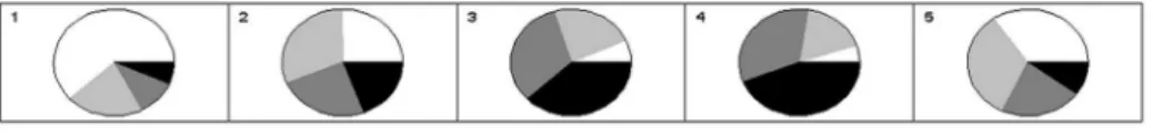
first classification C1. Fig. 5 shows the 5 code-vectors obtained by using a one-dimensional Kohonen algorithm with 5 units, classification C2. We see that the code-vectors of C1 and C2 are similar, and that the clusters are more or less ordered according to the housing expenses.
Fig. 4. The 5 code-vectors for classification C1.
Fig. 5. The 5 code-vectors for classification C2.
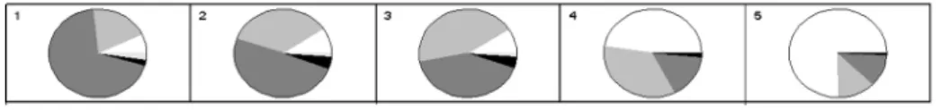
We can represent the distribution of the 4 levels of income across the 5 classes, in the classification C2, see Fig 6. In the same way, we study the distribution
Fig. 6. Distribution of the 4 income levels over the 5 classes of C2, 4 quartiles from white (low) to black (high).
of the residency status, which has 5 modalities: owner without mortgage, owner with mortgage, tenant, future owner tenant, owner becoming tenant. See Fig 7. Briefly, we can describe the 5 clusters of C2 from the left to the right. Cluster 1 gathers quasi-poor tenants with low income and the head of family is unem-ployed. Cluster 2 groups future owner tenant, with part time job. In cluster 3, one founds managers who are owner without mortgage, whore are less than 45 and are quasi-rich or rich. Cluster 4 contains fairly rich workers who own their house. In cluster 5 there are old persons who are owners, but who are poor with a low education level. The housing expenses are decreasing from cluster 1 to cluster 5, while low income consumers correspond to clusters 1, 2, 5 and high income consumers belong to clusters 3 and 4. The tenants are in clusters 1 and 2, the owners are in the others.
In order to evaluate the performance of the allocation algorithm, we deter-mine: 1) the ”true” class of each individual in the test set (by comparing its Y1, Y2, . . . , Yl vector with the code-vector of each cluster);
2) the cluster for which the probability computed in section 4 is maximum. We consider the contingency tables that match these two classifications. The sum of the diagonal entries is the number of exact allocations. We can also compute the number of times when the algorithm allocates the same cluster or its neighbors to the individuals of the test set. This number is the sum of
Fig. 7.Distribution of the 5 residency status modalities over the 5 classes of C2, tenant (medium grey) have majority in class 1, while owner without and with mortgage (white and light grey) are predominant in classes 3, 4 and 5 .
the entries of the diagonal and of the entries just above or just below. It is the number of correct allocations.
In the next table, the lines correspond to the allocation procedure and the columns to the exact classification C1.
Cluster 1 Cluster 2 Cluster 3 Cluster 4 Cluster 5 Total Allocated to 1 55 22 29 11 6 123 Allocated to 2 23 22 14 9 4 72 Allocated to 3 17 11 59 26 9 122 Allocated to 4 2 2 2 3 4 13 Allocated to 5 6 4 7 15 47 79 Total 103 61 111 64 70 409 From this table, we conclude that the number of exact allocations is 186, and the number of correct allocations is 186 + 117, that is 303, which represents 74% of the test set.
We can consider the same table for classification C2.
Cluster 1 Cluster 2 Cluster 3 Cluster 4 Cluster 5 Total Allocated to 1 33 12 3 3 5 56 Allocated to 2 23 33 22 17 3 98 Allocated to 3 8 27 56 15 3 109 Allocated to 4 0 3 11 42 21 77 Allocated to 5 8 3 1 10 47 69 Total 72 78 93 87 79 409 The number of exact allocations is 211, and the number of correct allocations is 186 + 141, that is 352, which represents 86% of the test set.
7
Conclusion
This paper proposes a simple method to study large databases which contain continuous and categorical variables at the same time, and to identify the cat-egory of an individual who is described by incomplete data. The results are convincing and it can give a very useful tool to decision-makers in many fields : insurance policies, personal tariffing, targeted advertising, credit scoring, etc.
8
Acknowledgement
The authors would like to thank Patrice Gaubert from SAMOS-MATISSE and Cr´eteil Universit´e for making the Canadian consumption data available to us, and the Gaz de France Company for partially funding this research via a previous partnership and collaboration on the allocations problem.
References
1. P.Allison(1999), Logistic Regression Using The SAS System. Theory and Applica-tion, Cary, NC, SAS Institute Inc.
2. M. Cottrell and P. Rousset, The Kohonen algorithm: a powerful tool for analysing and representing multidimensional quantitative et qualitative data, Proc. IWANN’97, Lanzarote, Springer, 861-871,
3. M. Cottrell, J.C. Fort, G. Pag`es (1998), Theoretical aspects of the SOM Algorithm, Neurocomputing, 21, 119-138.
4. M. Cottrell and P. Letr´emy (2005), Missing values: processing with the Kohonen algorithm, Proc. ASMDA, http://asmda2005.enst-bretagne.fr, Brest, 489-496. 5. M. Cottrell, P. Gaubert, P. Letr´emy, P. Rousset (1999), Analyzing and
represent-ing multidimensional quantitative and qualitative data: Demographic study of the
Rh¨one valley. The domestic consumption of the Canadian families, WSOM’99, In:
Oja E., Kaski S. (Eds), Kohonen Maps, Elsevier, Amsterdam, 1-14.
6. E. de Bodt, M. Cottrell, P. Letr´emy, M. Verleysen (2003), On the use of self-organizing maps to accelerate vector quantization, Neurocomputing, 56, 187-203. 7. S. Ibbou (1998), Classification, analyse des correspondances et m´ethodes
neu-ronales, PhD Thesis, Universit´e Paris 1-Panth´eon-Sorbonne.
8. (1997), S. Kaski (1887), Data Exploration Using Self-Organizing Maps, Acta Poly-technica Scadinavia, Mathematics, Computing and Management in Engineering
Series, N◦82 (D. Sc. Thesis, Helsinki, University of Technology).
9. T.Kohonen (1984), Self-Organization and Associative Maps, Springer Series in In-formation Sciences, Vol 8, Springer
10. T.Kohonen (1995), Self-Organizing Maps, Springer Series in Information Sciences, Vol 30, Springer.
11. P.Letr´emy, M.Cottrell, E.Esposito, V.Laffite and S.Showk (2005), The ”profilo-graph”: a toolbox for the analysis and the segmentation of gas load curves, Proc. WSOM 05, 447-454.
12. G.Maddala (1983), Limited-dependent and qualitative variables in econometrics, Cambridge University Press.
13. E.Oja, S.Kaski (1999), Kohonen Maps, Elsevier.
14. C.R. Rao (1973), Linear Statistical Inference and its applications, 2nd ed., Wiley, New-York.
15. P. Schmidt, R.P.Strauss (1975), The Prediction of Occupation Using Multiple Logit Models International Economic Review, vol. 16, no 2.