Comparison of GOME tropospheric NO₂ columns with NO₂ profiles deduced from ground-based in situ measurements

HAL Id: hal-00295996

https://hal.archives-ouvertes.fr/hal-00295996

Submitted on 3 Aug 2006

HAL is a multi-disciplinary open access

archive for the deposit and dissemination of

sci-entific research documents, whether they are

pub-lished or not. The documents may come from

teaching and research institutions in France or

abroad, or from public or private research centers.

L’archive ouverte pluridisciplinaire HAL, est

destinée au dépôt et à la diffusion de documents

scientifiques de niveau recherche, publiés ou non,

émanant des établissements d’enseignement et de

recherche français ou étrangers, des laboratoires

publics ou privés.

NO2 profiles deduced from ground-based in situ

measurements

D. Schaub, K. F. Boersma, J. W. Kaiser, A. K. Weiss, D. Folini, H. J. Eskes,

B. Buchmann

To cite this version:

D. Schaub, K. F. Boersma, J. W. Kaiser, A. K. Weiss, D. Folini, et al.. Comparison of GOME

tropospheric NO2 columns with NO2 profiles deduced from ground-based in situ measurements.

At-mospheric Chemistry and Physics, European Geosciences Union, 2006, 6 (11), pp.3211-3229.

�hal-00295996�

www.atmos-chem-phys.net/6/3211/2006/ © Author(s) 2006. This work is licensed under a Creative Commons License.

Chemistry

and Physics

Comparison of GOME tropospheric NO

2

columns with NO

2

profiles

deduced from ground-based in situ measurements

D. Schaub1, K. F. Boersma2, J. W. Kaiser3, A. K. Weiss1, D. Folini1, H. J. Eskes2, and B. Buchmann1

1_{Empa, Swiss Federal Laboratories for Materials Testing and Research, Ueberlandstrasse 129, CH-8600 Duebendorf,}

Switzerland

2_{Royal Netherlands Meteorological Institute (KNMI), P.O. Box 201, 3730 AE, De Bilt, The Netherlands} 3_{European Centre for Medium-Range Weather Forecasts (ECMWF), Shinfield Park, Reading, RG2 9AX, UK}

Received: 10 January 2006 – Published in Atmos. Chem. Phys. Discuss.: 31 March 2006 Revised: 23 June 2006 – Accepted: 28 July 2006 – Published: 3 August 2006

Abstract. Nitrogen dioxide (NO2) vertical tropospheric

column densities (VTCs) retrieved from the Global Ozone Monitoring Experiment (GOME) are compared to coincident ground-based tropospheric NO2columns. The ground-based

columns are deduced from in situ measurements at different altitudes in the Alps for 1997 to June 2003, yielding a unique long-term comparison of GOME NO2VTC data retrieved by

a collaboration of KNMI (Royal Netherlands Meteorologi-cal Institute) and BIRA/IASB (Belgian Institute for Space Aeronomy) with independently derived tropospheric NO2

profiles. A first comparison relates the GOME retrieved tro-pospheric columns to the trotro-pospheric columns obtained by integrating the ground-based NO2measurements. For a

sec-ond comparison, the tropospheric profiles constructed from the ground-based measurements are first multiplied with the averaging kernel (AK) of the GOME retrieval. The second approach makes the comparison independent from the a pri-ori NO2 profile used in the GOME retrieval. This allows

splitting the total difference between the column data sets into two contributions: one that is due to differences between the a priori and the ground-based NO2 profile shapes, and

another that can be attributed to uncertainties in both the re-maining retrieval parameters (such as, e.g., surface albedo or aerosol concentration) and the ground-based in situ NO2

profiles. For anticyclonic clear sky conditions the compari-son indicates a good agreement between the columns (n=157, R=0.70/0.74 for the first/second comparison approach, re-spectively). The mean relative difference (with respect to the ground-based columns) is −7% with a standard devia-tion of 40% and GOME on average slightly underestimating the ground-based columns. Both data sets show a similar seasonal behaviour with a distinct maximum of spring NO2 Correspondence to: D. Schaub

(daniel.schaub@empa.ch)

VTCs. Further analysis indicates small GOME columns be-ing systematically smaller than the ground-based ones. The influence of different shapes in the a priori and the ground-based NO2 profile is analysed by considering AK

informa-tion. It is moderate and indicates similar shapes of the pro-files for clear sky conditions. Only for large GOME columns, differences between the profile shapes explain the larger part of the relative difference. In contrast, the other error sources give rise to the larger relative differences found towards smaller columns. Further, for the clear sky cases, errors from different sources are found to compensate each other par-tially. The comparison for cloudy cases indicates a poorer agreement between the columns (n=60, R=0.61). The mean relative difference between the columns is 60% with a stan-dard deviation of 118% and GOME on average overestimat-ing the ground-based columns. The clear improvement after inclusion of AK information (n=60, R=0.87) suggests larger errors in the a priori NO2 profiles under cloudy conditions

and demonstrates the importance of using accurate profile in-formation for (partially) clouded scenes.

1 Introduction

Nitrogen dioxide (NO2)is one of the most important air

pol-lutants in the troposphere. It directly affects human health and plays a major role in the production of ground-level ozone (Seinfeld and Pandis, 1998; Finlayson-Pitts and Pitts, 2000). Furthermore, Solomon et al. (1999) pointed out the climatic effect of NO2as an absorber of solar radiation.

The bulk of the emitted NOx (≡NO+NO2)is of

anthro-pogenic origin (Brasseur, 2003). The primarily emitted ni-trogen oxide (NO) oxidises to NO2within seconds to

min-utes. The latter is removed from the troposphere after being

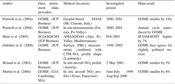
Table 1. Recent works on validation and/or intercomparison of space-borne NO2vertical tropospheric column densities with independent

measurement data.

Author Data:

instru-ment (data

provider)

Method (location) Investigated

period

Main result

Petritoli et al. (2004) GOME (IUP

Bremen)

Ground-based DOAS

(Mt. Cimone, Italy)

2000–2001 GOME smaller by 14%

Petritoli et al. (2004) GOME (IUP

Bremen)

In situ measurements (Fer-rara, Po-Valley)

2000–2001 Annual cycle

repro-duced by GOME

Heue et al. (2005) SCIAMACHY

(IUP Bremen)

AMAXDOAS (Alps, Po-Valley, Mediterranean)

Feb 2003 SCIAMACHY higher

by 7%

Ord´o˜nez et al. (2006) GOME (IUP

Bremen)

Surface (PBL)

measure-ments combined with

CTM-NO2 profile shape

(Lombardy)

1996–2002 GOME best agrees for

slightly polluted sta-tions

Heland et al. (2002) GOME (IUP

Bremen)

In situ aircraft NO2profile

(Austria)

2 May 2001 GOME smaller by 3%

Martin et al. (2004) GOME (CfA

Cambridge, MA)

In situ aircraft NO2

pro-files (Texas, Tennessee)

June/July 1999

Aug/Sep 2000

GOME smaller by 8%

converted to nitric acid (HNO3)which deposits (Kramm et

al., 1995). During daytime, HNO3 is formed through the

reaction of NO2 with the OH radical. During night time,

a two step reaction chain forms nitrogen pentoxide (N2O5).

The latter further reacts on surfaces and aerosol to HNO3

(Dentener and Crutzen, 1993). The resulting NOxlifetime is

highly variable with an annual average boundary layer life-time in the order of one day (Warneck, 2000). During photo-chemically active summer days, the lifetime can be reduced to only a few hours (e.g. Spicer, 1982). An increasing life-time up to several days is found with increasing height in the troposphere (Jaegl´e et al., 1998; Seinfeld and Pandis, 1998; Warneck, 2000). The mainly near-ground emissions of ni-trogen species over industrialised areas, their production and loss reactions and meteorological transport lead to a distinct vertical tropospheric profile of NO2 with enhanced mixing

ratios in the polluted boundary layer.

In terms of air quality in Switzerland, the NOxpollution

situation has been improved during the last 15 years, but the annual limit values are still exceeded in polluted areas (BUWAL, 2004). Therefore, monitoring of nitrogen oxides still plays an important role in order to examine reduction measures. In addition to the monitoring networks around the globe, which provide ground-based in situ NO2

measure-ments, space-borne spectrometers such as GOME (Burrows et al., 1999) provide area-wide information about the NO2

vertical tropospheric column densities (VTCs) with a global coverage within only a few days.

1.1 Previous validation or comparisons studies with space-borne NO2VTCs

Typically, for validation purposes, space-borne trace gas columns are compared to ground-based or airborne column

measurements. Some recent works on validation of NO2

VTCs are summarised in Table 1. The comparison of GOME NO2 VTCs with ground-based DOAS measurements

car-ried out at Mount Cimone (Italy) yielded a good agreement for situations with horizontally homogeneous distribution of the pollution distribution (Petritoli et al., 2004). Heue et al. (2005) used the Airborne Multi Axis DOAS (AMAX-DOAS) instrument on board the DLR Falcon to validate SCIAMACHY (Scanning Imaging Absorption Spectrometer for Atmospheric Chartography; Bovensmann et al., 1999) NO2 VTCs over Italy in February 2003 and found

SCIA-MACHY values to be systematically higher than AMAX-DOAS by approximately 7%.

Few comparisons including in situ data can be found in literature. The fundamental problem when comparing in situ measurements with column quantities arises from the fact that the latter integrate both horizontally and vertically, whereas in situ measurements provide point (ground-based site) or line (aircraft profile) information only. Petritoli et al. (2004) compared boundary layer in situ measurements from the Po-valley with GOME NO2 VTCs and found a

good qualitative correlation in the annual trend for high pol-lution episodes. Ord´o˜nez et al. (2006) used 3-monthly av-eraged profile shapes from the chemistry transport model (CTM) MOZART-2 (Horowitz et al., 2003) that are scaled with ground-based in situ measurements for comparison with GOME NO2VTCs in the Lombardy region (Italy). Because

the GOME NO2 VTCs used in that study were retrieved

based on a priori profiles from the same CTM, the focus has been on finding the best average boundary layer pollution level that scales the CTM column to best fit the GOME mea-surements. The best agreement has been found for average polluted situations.

In a case study, one in situ NO2profile measured from the

DLR Falcon on a clear sky day above Austria has been used by Heland et al. (2002) for a comparison with GOME. They found a very small difference of −0.1×1015molec cm−2 be-tween the GOME and the in situ column. Martin et al. (2004) evaluated the consistency between GOME tropospheric NO2

columns and averaged aircraft profile measurements not co-inciding with the GOME observation. The latter two com-parisons are the only published comcom-parisons of tropospheric GOME NO2observations with independent tropospheric in

situ profile measurements known to the authors. Further-more, the comparison case study by Heland et al. (2002) is the only study that validates an individual GOME retrieval with a coincident aircraft profile.

Shortcomings of the validations/comparisons mentioned above arise from their necessary focus on very limited num-bers of coincident pixels (or even single pixels) or their use of CTM derived NO2profile shapes. Furthermore, no study

so far discussed the inclusion of averaging kernels for the comparison of space-borne NO2 VTCs with independently

derived NO2columns.

1.2 Present study

The present study compares GOME NO2VTCs from 1997

to June 2003 with a set of NO2columns derived from in situ

NO2 measurements in Switzerland. Ground-based in situ

sites continuously measuring NO2at different altitudes in the

Alpine region are used to obtain tropospheric NO2profile

in-formation. New aspects of the present work are

– the first long-term comparison of GOME NO2 VTC

data retrieved by KNMI/BIRA (available at the Tropo-spheric Emission Monitoring Internet Service (TEMIS) web site http://www.temis.nl) with independently de-rived tropospheric NO2profiles,

– the NO2 profile/column construction from

ground-based in situ measurements,

– the comparison through inclusion of averaging kernel information,

– the first investigation of tropospheric NO2retrieval

er-rors under cloudy situations.

Both the space-borne and the ground-based in situ measure-ment data are described in Sect. 2. The detailed method of deducing the tropospheric NO2 column from ground-based

in situ measurements is introduced in Sect. 3. Sections 4 and 5 discuss the ground-based in situ columns (hereafter called ground-based columns) and the comparison between the lat-ter and GOME NO2VTCs for anticyclonic clear sky and for

cloudy conditions, respectively.

2 Measurement data

2.1 KNMI/BIRA GOME tropospheric NO2observations

The Global Ozone Monitoring Experiment (GOME) instru-ment on board ESA’s ERS-2 satellite is a nadir-viewing spec-trometer that measures upwelling radiance from the atmo-sphere and solar irradiance. The satellite instrument takes observation at approximately 10:30 h local time and individ-ual pixels cover an area of 320×40 km2. The GOME princi-ples are described by Burrows et al. (1999).

The GOME NO2VTCs studied in this work are the result

of a collaboration of KNMI and BIRA/IASB. GOME NO2

data are publicly available on a day-by-day basis from 1 April 1996 until 30 June 2003 via ESA’s TEMIS project (http:// www.temis.nl).

The first step of the retrieval is taken by BIRA/IASB based on the Differential Optical Absorption Spectroscopy (DOAS) technique (Vandaele et al., 2005). It consists of the fitting of a modelled spectrum to a GOME-measured reflectance spectrum in the spectral window from 426.3–451.3 nm. This modelled spectrum takes into account the spectral features of absorption by NO2, O3, O2-O2and H2O, and describes

scat-tering on clouds, aerosols and air molecules by a low-order polynomial. The result of this first step is the so-called slant column density (SCD) of NO2. This SCD should be

inter-preted as the column integral of absorbing NO2 molecules

along the effective photon path from the sun through the at-mosphere to the GOME spectrometer.

The second step of the retrieval is the separation of the stratospheric contribution from the total SCD (Boersma et al., 2004). This is achieved with a data-assimilation ap-proach. In the data-assimilation step, NO2in TM4 (Dentener

et al., 2003) is made consistent with observed SCDs over un-polluted areas. Subsequently, the stratospheric estimate is subtracted from the total SCD. Note that the residual tropo-spheric slant column (SCDtrop)is insensitive to calibration

errors, as any offsets in the total and stratospheric SCDs will cancel in the subtraction. Finally, the SCDtrop is converted

into a VTC by applying the tropospheric air mass factor. The latter is calculated with the Doubling Adding KNMI (DAK) radiative transfer model (Stammes, 2001) and represents the best estimate of the length of the effective photon path for a particular retrieval scene. The tropospheric air mass fac-tor depends on a priori assumptions on the state of the atmo-sphere, including surface albedo, cloud fraction, cloud height and the vertical distribution of NO2. For KNMI retrievals, a

priori NO2profiles for every location and all times are

ob-tained from the TM4 CTM. Cloud parameters are taken from the Fast Retrieval Scheme for Clouds from the Oxygen A band (FRESCO) algorithm (Koelemeijer et al., 2001).

During the above mentioned steps, a number of error sources can lead to inaccurate retrieval results. The error budget of the tropospheric vertical columns has been studied extensively in Boersma et al. (2004). Over polluted regions

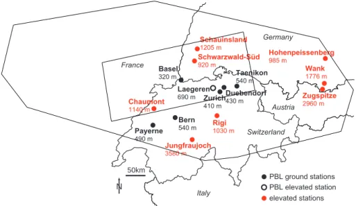
50km N Payerne 490 m Laegeren 690 m Taenikon 540 m Jungfraujoch 3580 m Rigi 1030 m Chaumont 1140 m Zugspitze 2960 m Wank 1776 m Duebendorf 430 m Austria Italy Germany France Switzerland Basel 320 m Bern 540 m Schauinsland 1205 m Hohenpeissenberg 985 m Schwarzwald-Süd 920 m Zurich 410 m PBL ground stations PBL elevated station elevated stations

Fig. 1. Ground-based in situ measurement stations in the PBL and at elevated sites used in the present study. GOME pixels with its centre

coordinates located within the rectangular frame above northern Switzerland are used for the comparison. The resulting region covered by the GOME pixels of interest is additionally denoted.

as considered in the present study, errors in the SCD (e.g. due to instrument noise, laboratory reference spectra errors, inter-ference with other absorbers and Ring effect) and in the sep-aration of the stratospheric contribution from the total SCD play a minor role. For such regions, the most critical error source is the calculation of the tropospheric air mass factor. The latter depends on the a priori assumed NO2profile shape,

the cloud fraction, the cloud top height, the surface spectral reflectance (surface albedo, e.g. near land-snow boundaries) and the aerosol optical thickness profile. Based on theoret-ical error sources and for cloud free conditions, Boersma et al. (2004) estimated mean tropospheric air mass factor un-certainties for polluted regions (>1.0×1015molec cm−2) of 15%, 2%, 15% and 9% due to the model parameters cloud fraction, cloud top height, surface albedo and a priori NO2

profile shape, respectively. The total mean uncertainty for the tropospheric air mass factor is estimated to be 29%, re-sulting in a total mean uncertainty for the NO2VTCs of 35–

60%. No error due to aerosol is included for the KNMI NO2

retrievals. Boersma et al. (2004) have argued that the pres-ence of aerosol modifies the retrieval of cloud fraction and height with the FRESCO algorithm. A comparison of the expected aerosol correction factor versus the actual correc-tion effect from the cloud retrieval has shown that even for a large aerosol optical thickness, the expected correction factor and actual correction effect agree to within 10%. Boersma et al. (2004) therefore suggest that cloud algorithms implicitly correct for aerosol through their modified cloud fraction and height.

Due to the cloud parameters that can be affected by un-certainties and the simplifying assumption that the cloud can be approximated as a Lambertian reflector with an effective

cloud top height, larger errors are expected for the retrieval of cloudy scenes. The DAK radiative transfer model (Stammes, 2001) accounts for multiple scattering, but a detailed quanti-tative error analysis has so far not been carried out for these issues. Preliminary simluations with the DAK showed that light penetrates quite far into the cloud and the NO2 signal

can originate from the upper half of the cloud. The FRESCO effective cloud top height represents this by putting the ef-fective reflective surface below the real cloud top. However, the above mentioned small error due to uncertainties in the cloud top height for clear sky conditions can be thought to increase when the clouds are associated with, e.g., frontal ac-tivity. The vertical mixing of near ground pollution can then lead to a higher NO2abundance near the cloud top, which

in-duces a larger error compared to the clear sky situation with the bulk of the NO2residing well below the cloud height. An

explicit quantification of the error of cloudy NO2VTCs has

so far not been given in literature, but we estimate it to be in the order of 100%.

2.2 Ground-based in situ measurements

The Swiss National Air Pollution Monitoring Network (NABEL) provides long-term ground-based in situ measure-ments. Planetary boundary layer (PBL) stations representa-tive for different pollution levels as well as stations located at different altitudes are included in this study (Fig. 1). In order to get more information about higher levels in the lower tro-posphere, two Alpine stations operated by the Umweltbunde-samt (Germany) are further taken into account (Fig. 1). De-tails about measurement devices and locations can be found in Umweltbundesamt (2003), BUWAL (2004) and Empa (2005).

NO2 is measured with the chemiluminescence technique

(Navas et al., 1997; Clemitshaw, 2004) that includes the con-version of NO2to NO. While the Jungfraujoch and the

Ho-henpeissenberg stations are equipped with photolysis con-verters that allow a selective measurement of NO2, the other

stations are measuring with the molybdenum conversion technique. It is known that these catalytic surface convert-ers are sensitive not only to NO2, but also to other nitrogen

species such as PAN, HNO2, HNO3 and particulate nitrate

(Zellweger et al., 2003; Clemitshaw, 2004). In order to ac-count for this non-selective NO2measurements at most of the

stations used in this study, campaign results of simultaneous measurements based on both the photolysis and the molyb-denum conversion technique at a PBL station (Taenikon) and an elevated station (Rigi) are used to determine correction factors (Sect. 3.1.3). A similar approach has been used in Ord´o˜nez et al. (2006).

3 Methods

3.1 Column calculation from ground-based in situ mea-surements

The mountainous terrain in the Alpine region allows oper-ating ground-based in situ measurement sites at different al-titudes. These stations are assumed to detect NO2

concen-trations that are approximately representative for the appro-priate height in the (free) troposphere over flat terrain. These measurements, together with boundary layer in situ measure-ments and an assumed mixing ratio at 8 km, are used to con-struct NO2profiles. The latter can subsequently be integrated

to tropospheric NO2columns. Deducing tropospheric profile

and column information from ground-based in situ measure-ments is not straightforward because the issue of representa-tiveness has to be taken into account carefully. The following subsection alludes to the principle method of constructing the NO2profile from the in situ measurements. Afterwards,

is-sues of representativeness and errors are discussed. 3.1.1 Deducing the NO2profile/column

The stations shown in Fig. 1 are used to deduce the tro-pospheric NO2 profile. Every station provides a 3-h NO2

average concentration calculated from 09:00 to 12:00 UTC (i.e. around the GOME overpass at 10:30 h local time). Con-centrations not measured with a photolysis converter are cor-rected with correction factors accounting for the interference in the NO2measurement (Sect. 3.1.3). Because we are

go-ing to use averaggo-ing kernel (AK) information with a higher vertical resolution than covered by the various stations, the ground-based profile is divided into partial subcolumns to match the vertical resolution of the AK.

The NO2 in the upper troposphere is neglected because,

due to the generally smaller mixing ratios and decreasing pressure with height, the effective NO2 molecule number

Table 2. NO2pollution classes represented by population density

ranges and associated representative Swiss Plateau (boundary layer) ground measurement stations.

Pollution class Population density Representative (c) [km−2] measurement station Very remote <30 None (0.5× remote) Remote 30–499 Taenikon, Payerne Polluted 500–999 Duebendorf, Basel Highly polluted >1000 Berne, Zurich

concentration at these levels is small compared to the NO2

in the lower troposphere (Sect. 3.1.2). The elevated stations (above 900 m a.s.l.) together with a near-zero NO2mixing

ratio of 0.02 ppb at 8 km are first used for a curve fit, which can be regarded as an average profile given by the elevated stations. The curve fit is based on a power law equation re-sulting in a hyperbolic profile shape. Subsequently, the in situ measurements are assigned to the appropriate height in-tervals in the following way:

Above 900 m a.s.l. (i.e. for the elevated part of the pro-file), the partial subcolumns are given as either the mean NO2concentration from the stations within the height

inter-val, or the NO2concentration from the curve fit if no elevated

station is available. Subcolumns for height intervals below 900 m a.s.l. are obtained from linear interpolation between the 900 m NO2 concentration (resulting from the curve fit)

and the remote and elevated PBL station Laegeren, as well as between the latter and the average PBL NO2

concentra-tion at the mean Swiss Plateau ground height of 400 m a.s.l. To determine the average PBL NO2concentration within

an individual GOME pixel, spatial inhomogeneities of the NOx emissions must be taken into account. To do this, we

assume that the NOxemissions are proportional to the

popu-lation density distribution. This assumption has previously been proven to be useful (Schaub et al., 2005). For the GOME pixel under consideration, the 0.25◦_×0.25◦ popula-tion density grid elements enclosed in the pixel are sorted into four different (arbitrarily chosen) pollution classes c (Ta-ble 2). Each class is described by a population density range and appropriate measurement stations representative for the pollution level (Empa, 2005). From the numbers pcof pop-ulation density grid elements in each class, the average PBL NO2concentration within the GOME pixel is calculated as a

weighted mean concentration using the appropriate stations representative for the pollution class:

[NO2]pbl = 4 P c=1 [NO2]c·pc 4 P c=1 pc .

Measurement gaps at the ground measurement sites occa-sionally prevent the use of all 15 stations from Fig. 1 for the NO2profile construction. On average, 13 stations are

avail-able for deducing a profile.

The ground-based columns described so far are derived for an NO2profile starting at ground-height (Swiss Plateau).

The Alpine terrain is excluded as far as possible (Fig. 1). Nevertheless, the GOME pixels always cover a non-flat ter-rain in the present study area and the signal can be seen as a superposition of signals associated with columns of dif-ferent vertical extension. To reproduce this in the ground-based columns, the topography of the Alpine Local Model (aLMo, operational numerical weather forecast model of MeteoSwiss) with a resolution of 7 km×7 km is used to cal-culate a mean (or effective) surface height within the GOME pixel. The part of the ground-based NO2VTC located above

this height is finally used as the representative ground-based column for the further comparison.

3.1.2 Representativity of the constructed profiles

The representativity of the profiles constructed by the method described in Sect. 3.1.1 for the true atmospheric NO2profile

over Northern Switzerland may be limited as a consequence of the following:

A) The vertical distribution of NO2 within the PBL may

not be well captured.

B) Inhomogeneities of NO2over the size of a GOME pixel

may not be well captured.

C) Elevated stations may not be representative for the NO2

at corresponding heights.

Here we shortly discuss each of these issues and their possi-ble impact on the representativity of our constructed profile. A) Vertical NO2distributions within the PBL are variable.

For instance, Pisano et al. (1997) have shown NO2to be

ho-mogeneously distributed within the well-mixed convective boundary layer (CBL) in summer. On the other hand, Her-wehe et al. (2000) modelled the boundary layer NO2

ver-tical distribution and found that also within a summertime well-mixed boundary layer, the NO2can exhibit a strong

de-crease with height because the NO2 lifetime can be shorter

than the typical mixing time scale in the CBL (Spicer, 1982; Herwehe et al., 2000). Therefore, in situ measurements from an additional PBL station that is located on a mountain ridge about 250 m above the ground height of the Swiss Plateau (Laegeren, Fig. 1) are used (Sect. 3.1.1).

B) Due to the distances between the elevated stations (Fig. 1) and the relatively short chemical lifetime of NO2it is

obvious that small-scale structures of the 3-dimensional NO2

distribution in the free troposphere are difficult to catch by our comparison approach. Furthermore, neglecting the upper troposphere NO2 above 8 km might not apply for columns

affected by lightning or deep convection where NO2column

enhancements of up to 1.0×1015molec cm−2_{were reported}

(Boersma et al., 2005; Choi et al., 2005). However, such events occur only occasionally and are not expected during anticyclonic clear sky days. During such conditions, Rid-ley et al. (1998) conducted simultaneous flights measuring NOx profiles up to 5000 metres asl representative locally

(flight patterns with sides of 15–20 km) and regionally (hor-izontal flight distances of around 200 km) and qualitatively described a good agreement between the two profiles. Al-though these measurements were carried out at lower lati-tudes (30◦ to 34◦N), we suggest that the focus on anticy-clonic conditions supports our assumption of the NO2being

homogeneously distributed on clear sky high pressure days also in mid latitudes.

It can be expected that larger inhomogeneities occur un-der cloudy conditions when frontal transport takes place. However, such conditions can also lead to spatially extended air masses, which are relatively well-mixed (Schaub et al., 2005). We furthermore note the large GOME footprint, which averages over a large area. Finally, the averaging time window for the ground-based measurements from 09:00– 12:00 UTC to a certain extent averages out horizontal inho-mogeneities.

C) Measurements from elevated stations may not be rep-resentative for the NO2 at corresponding heights over flat

terrain. It is known that, mainly during summertime con-vective conditions in the Alpine region, even high-alpine sta-tions often detect pollution that reaches the site due to ther-mally induced upslope transport in the afternoon (Forrer et al., 2000; Lugauer et al., 2000; Nyeki et al., 2000; Zell-weger et al., 2003). However, because of the GOME over-pass around 10:30 h local time in the morning with an aver-aging time window for the ground-based in situ NO2

mea-surements from 09:00–12:00 UTC, this is not expected to be a major issue for the present comparison. During the winter season, high-alpine sites have shown to be decoupled from the boundary layer during anticyclonic conditions, and thus representing the undisturbed free troposphere (Lugauer et al., 2000). Hence, we expect the high-alpine measurements taken during the GOME overpass time to be representative for free tropospheric NO2levels.

Stations located around 1000 m a.s.l., on the other hand, are affected by polluted air masses already before noon. Nevertheless, we suggest these stations to be representative. Three cases can be distinguished:

1) On clear sky summer days, the boundary layer height grows very fast and can reach heights of 1000 m above ground already before noon (Nyeki et al., 2000; Seibert et al., 2000). Because in Switzerland a station located at 1000 m a.s.l. lies around 500 m above the ground (Swiss Plateau) effectively, the site can be thought to represent the PBL NO2levels.

2) During wintertime, the PBL often does not reach a height of 500 m above ground (e.g. Seibert et al., 2000).

In fact, the stations around 1000 m a.s.l. used in this study often measure low concentrations during clear sky winter days. Therefore, in winter, measurements at 1000 m a.s.l. are thought to be representative for free tropospheric NO2levels.

3) In spring, the upslope pollution transport could lead to pollution located above the PBL height over flat terrain, and one might argue that a station is no longer representa-tive for the corresponding height level over the flat terrain. On the other hand, GOME measurements over the northern part of Switzerland should detect such events to a certain ex-tent. The region is surrounded by mountainous areas with the Alps and the foothills of the Alps in the south/east and the Jura/Black Forest mountains in the north. Lugauer et al. (1998) argued that pollution once lifted can reside in the free troposphere. A measurement site affected by thermal upslope pollution transport can therefore be regarded to be representative for the “disturbed” free troposphere on a re-gional scale at least. Thus, with the five measurement sites around 1000 m a.s.l. and situated at five different locations within the region of interest and with different slope expo-sitions and surroundings included in this study, the overall pollution situation should – on average – be captured. Nev-ertheless, NO2concentration differences between these five

measurements are taken as a measure for inhomogeneities and thermally induced upslope transport (Sect. 3.1.4). 3.1.3 Interference in ground-based in situ NO2

measure-ments

Ground measurement stations equipped with molybdenum converters overestimate the NO2 concentration due to

non-selective conversion of nitrogen species (Clemitshaw, 2004). Due to the complex chemistry of nitrogen species, the dif-ference between the selective and the non-selective NO2

measurement strongly depends on meteorological conditions and the distance of the station from major emission sources. Campaign results of two stations that simultaneously mea-sured with both the photolysis (selective NO2measurement)

and the molybdenum conversion technique (non-selective NO2 measurement) are used to compute a correction

fac-tor: a boundary layer station (Taenikon, 540 m a.s.l.) and an elevated site (Rigi, 1030 m a.s.l.) for the correction of measurements from boundary layer and elevated stations, re-spectively. The correction factor is calculated as

cf = [NO2]photolysis [NO2]molybdenum

.

The elevated stations at Jungfraujoch and Hohenpeissenberg are equipped with selective (photolysis) converters and are, therefore, not corrected. Due to the seasonal variation in the photochemical activity monthly averaged correction fac-tors are calculated for NO2 measurements from 09:00 to

12:00 UTC (Fig. 2). 0 0.2 0.4 0.6 0.8 1 Month N O2 (p h o to ly s is )/ N O2 (m o ly b d e n u m )

Feb ÞA Oct Dez

ug J ß un A Þ pr a Rigi, 1030 m asl 0 0.2 0.4 0.6 0.8 1 Month N O2 (p h o to ly s is )/ N O2 (m o ly b d e n u m )

Feb ßJ Aug Oct Dez

un Apr b T à aenikon, 540 m asl

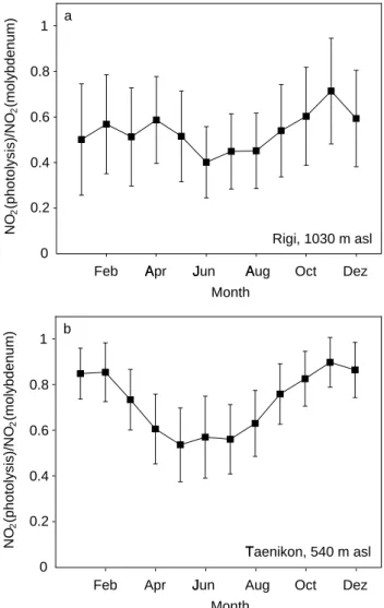
Fig. 2. Monthly mean ratios (and standard deviations) between NO• concentrations measured from 09:00 to

12:00 UTC on clear sky days with photolysis and with molybdenum conversion technique for the elevated station Rigi (a) and the PBL station Taenikon (b).

35

Feb ÞA Oct Dez

ug J ß un A Þ pr a Rigi, 1030 m asl 0 0.2 0.4 0.6 0.8 1 Month N O2 (p h o to ly s is )/ N O2 (m o ly b d e n u m )

Feb ßJ Aug Oct Dez

un Apr b T à aenikon, 540 m asl

Fig. 2. Monthly mean ratios (and standard deviations) between NO• concentrations measured from 09:00 to

12:00 UTC on clear sky days with photolysis and with molybdenum conversion technique for the elevated station Rigi (a) and the PBL station Taenikon (b).

35

Fig. 2. Monthly mean ratios (and standard deviations) between NO2

concentrations measured from 09:00 to 12:00 UTC on clear sky days with photolysis and with molybdenum conversion technique for the elevated station Rigi (a) and the PBL station Taenikon (b). 3.1.4 Error estimation for ground-based NO2VTCs

This section discusses the main error sources in the ground-based columns and suggests a simple “worst case” error es-timate.

1) The error due to the selected pollution classes for deter-mining the average PBL NO2concentration (Sect. 3.1.1) is

very small. This is because the weak impact due to chang-ing pollution classes is further decreased by the use of an effective surface height at the GOME pixel location. The effective surface height does not reach down to the Swiss Plateau height. Based on different choices for the pollution classes, relative uncertainties in the resulting ground-based NO2 VTCs of only a few percent are found. This error is

very small compared to the other errors and is therefore ne-glected.

2) Errors in the vertical NO2distribution in the PBL, the

representativity of elevated stations for the free troposphere,

and the assumption of horizontal homogeneity of NO2in the

free troposphere as discussed in Sect. 3.1.2 can be thought to be a major error source for the estimated ground-based columns. A crude overall estimation of this error is based on the five measurement sites located at altitudes of between 920 m a.s.l. and 1205 m a.s.l. (Fig. 1). On the one hand, these sites strongly affect the NO2profile deduced from the ground

stations. On the other hand, the stations are located in an al-titude range of only 285 m. Therefore, the standard deviation of their NO2concentrations is taken as an indicator for

hor-izontal inhomogeneities and the non-representativeness of certain stations due to, e.g., thermal upslope transport of pol-lution. The resulting uncertainty of the ground-based column is determined with a sensitivity test, where the five concentra-tions are enhanced simultaneously by the calculated standard deviation. This can be seen as a “worst case” scenario. The average resulting uncertainty is in the order of 20%, with an upper limit of approximately 50%.

3) Another significant error arises from the non-selective NO2 measurement techniques used at most of the ground

stations. Correction factors calculated for a selected station might not be representative for another station. Furthermore, meteorological conditions affect the correction factor, as in-dicated by the large standard deviations in the monthly cor-rection factors (Fig. 2). For the error estimation, the change in the ground-based columns is calculated with monthly cor-rection factors that are simultaneously changed by their stan-dard deviations (“worst case” scenario). The average result-ing error is in the order of 30%, with an upper limit of ap-proximately 35%.

Finally, because dependence between these errors cannot be excluded, the error is assumed to be additive and is calcu-lated as the sum of the two main error contributions, amount-ing to a conservative estimate of the average error of around 50%. This error will consist of both systematic error butions – which will amount to a bias – and random contri-butions. The same holds for the GOME retrievals.

3.2 Space-borne to ground-based comparison methods Following Palmer et al. (2001) and Boersma et al. (2004), the retrieved GOME NO2VTC (V T CGOME)is calculated as

V T CGOME= SCDtrop AMFtrop(xa,b) = SCDtrop· P lxa,l P lml(b) · xa,l . (1)

SCDtrop denotes the tropospheric slant column density,

which is the difference between the total SCD resulting from fitting the reflectance spectrum measured from the satellite and a stratospheric SCD. For KNMI retrievals, the latter is determined by data assimilation of observed SCDs in a chemistry-transport model (Eskes, 2003). AMFtrop is the

tropospheric air mass factor, which is defined as the ratio be-tween SCD and VTC. xa,l are the layer specific subcolumns from the a priori profile xa, and mlare the altitude-dependent scattering weights. The latter are calculated with a radiative

transfer model and best estimates for forward model parame-ters b, describing surface albedo, cloud parameparame-ters (fraction, cloud top pressure) and GOME pixel surface pressure.

If independently measured tropospheric NO2profile

infor-mation xind is available, there are different possibilities for

comparison, each having its own meaning. 3.2.1 First comparison approach

The straightforward first comparison approach (hereafter called first comparison) uses the independently measured NO2 profiles that are directly integrated to tropospheric

columns (V T Cind):

V T Cind=

X

lxind,l, (2)

with xind the ground-based NO2 profile and l the

tropo-spheric layers. The relative difference between the two columns with respect to the ground-based column is calcu-lated as

10=V T CGOME_{V T C}−V T Cind

ind

=f (SCDtrop, ml(b), xa,xind).

(3) 10is a measure that will be comparable to other validation

studies where, typically, relative differences are calculated with respect to the “true” columns. 10 depends on all

pa-rameters affecting the retrieval and the ground-based column calculation, including differences in the shapes of the a priori profile xaand the ground-based profile xind.

A second relative difference is calculated with respect to the GOME column (and the latter therefore being the denom-inator in Eq. 4):

11=V T C_{V T C}GOME−V T Cind

GOME

=f (SCDtrop, ml(b), xa,xind).

(4) The reason for defining 11will become obvious in the next

section (where 11is further divided into two contributions).

3.2.2 Second comparison approach

Eskes and Boersma (2003) applied the general formalism de-veloped by Rodgers (2000) for the case of DOAS retrievals that are typically done for weak absorbers (τ <1) and gener-ally give column integrals of the concentration species only. The averaging kernel (AK) vector describes the relation be-tween the true vertical distribution of a species and the re-trieved vertical column. Multiplying the ground-based NO2

profile with the AK yields V T Cind AK:

V T Cind AK =

X

lal(xa,b) · xind,l, (5) with al the AK element for layer l. Following Boersma et al. (2004) the relative difference between V T Cind AK and

the GOME column is

12=V T CGOME_{V T C}−V T C_GOMEind AK

=f (SCDtrop, ml(b), xind).

Unlike 11, 12 is no longer influenced by the a priori NO2

profile xa(Eskes and Boersma, 2003). For the interpretation of the second comparison approach (hereafter called second comparison), it is helpful to reformulate Eq. (6). Following Eskes and Boersma (2003), the expression for alcan be writ-ten as

al =

ml(b) AMFtrop(xa,b)

. (7)

Including Eqs. (1), (5) and (7) in Eq. (6) and reformulating yields 12= SCDtrop−Plml(b)·xind,l SCDtrop =f (SCDtrop, ml(b), xind). (8) Equation (8) demonstrates that the second comparison amounts to a comparison of slant column densities. Be-cause the AMFtrop divides out, the a priori NO2profile xa no longer contributes to 12. Further, the second term of

the numerator in Eq. (8) indicates the slant column to be a linear sum of signal contributions from all individual layers, which is a valid approximation for weak absorbers (Eskes and Boersma, 2003; Boersma et al., 2004). Therefore, the above equation can be interpreted as how well the ground-based NO2 profile together with the scattering weights ml can describe SCDtrop.

In the previous section, we introduced 11, which depends

on all parameters affecting the comparison. Because the same denominator appears in both 11and 12, we can write

11=12+13. (9)

Therefore, 11 can be split into two contributions: 13 that

depends on differences between the shapes of the a priori and the ground-based NO2profile, and 12that is due to

un-certainties in both the remaining retrieval parameters and the ground-based NO2profile. In the following, 11and 12are

calculated from the first and the second comparison, respec-tively. 13 is calculated as the difference between 11 and

12.

4 Results for clear sky (anticyclonic) conditions

4.1 NO2VTCs from ground-based in situ measurements

From 1997 to June 2003, ground-based NO2VTCs are

cal-culated for 335 days with both clear sky conditions (Me-teoSwiss, 1985) and GOME NO2VTC data above northern

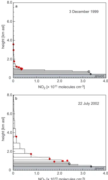
Switzerland (Fig. 1) available. Figure 3 shows two exam-ple NO2 profiles deduced from ground-based in situ

mea-surements for 3 December 1999 and for 22 July 2002. The December example shows a typical anticyclonic winter case where an inversion prevents vertical mixing and the NO2is

concentrated in the narrow PBL. The more effective mix-ing in the July example and the reduced chemical lifetime of NO2 during the warm season leads to a boundary layer

1.0 3.0 4.0 0 2.0 4.0 6.0 8.0 0 NO₂ [x 1011 _{molecules cm}-3_] height [km asl] 2.0 3 December 1999 ground a 1.0 3.0 4.0 0 2.0 4.0 6.0 8.0 0 NO₂ [x 1010 _{molecules cm}-3_] height [km asl] 2.0 22 July 2002 b ground

Fig. 3. Example NO2profiles for 3 December 1999 (a) and for

22 July 2002 (b). Note the different x-axis. The two PBL values (filled and open black circles) are derived from the PBL ground and elevated stations in Fig. 1. The red data points are derived from the elevated stations located in Southern Germany and Switzerland (Fig. 1). Occasionally, measurement gaps prevent the use of all available measurement sites for the profile determination.

concentration being a factor of 10 lower than for the winter case.

Employing 12:00 UTC radio soundings from Payerne (Switzerland; e.g. Beyrich et al., 1998), PBL heights are calculated with the parcel method (Troen and Mahrt, 1986; Holtslag et al., 1990) and the Richardson number method (Vogelezang and Holtslag, 1996). With these PBL heights, the annual mean fractions of NO2located within and above

the PBL are calculated to be 69% and 31%, respectively, for the ground-based NO2profiles reaching down to the Swiss

Plateau height. For comparison, Martin et al. (2004) reported a summertime fraction of nearly 75% of the tropospheric

Table 3. Fraction of NO2 vertical column density (VTC) above

and within the planetary boundary layer (PBL) calculated from the ground-based NO2VTC alone and multiplied with averaging

ker-nel (AK) information. The whole ground-based NO2columns are

considered (i.e. reaching down to the height of the Swiss Plateau). Ground-based Ground-based NO2VTC NO2VTC×AK

Fraction of NO2above PBL 31±14% 55±16%

Fraction of PBL NO2 69±14% 45±16%

NO2below 1500 m in Houston and Nashville, USA. Ord´o˜nez

et al. (2006) found an average NO2fraction below 1000 m

in the northern Italy region of more than 80%. The rea-son for the lower PBL column fraction in the area of north-ern Switzerland and surroundings is the lower NO2pollution

compared to northern Italy.

The GOME nadir UV-VIS sensor exhibits a higher sensi-tivity towards NO2located in higher atmospheric layers. To

check the “satellite’s view”, the layer-specific NO2 (xind,l)

is multiplied with the altitude-dependent scattering weight ml to get the within/above PBL NO2 SCDs as seen from

satellite. Employing averaging kernel information and the AMFtropand following Eq. (7) in Sect. 3.2.2 the NO2SCD

above the PBL is SCDNO2above PBL = P above PBL xind,l·ml(b) =AMFtrop· P above PBL xind,l·al. (10)

Similarly the total tropospheric NO2 SCD, the PBL NO2

SCD and, subsequently, the fractions within and above the PBL are calculated. Table 3 indicates that, on average, 55% of the signal measured by the space-borne instrument in the present study area originates from above the PBL, although only 31% of the NO2resides there in reality. The PBL

con-tribution is 45%. Because the following comparison employs the part of the ground-based profile located above the mean topography height within a GOME pixel, the importance of the PBL contribution is further reduced. This emphasises the importance of the elevated stations for the present compari-son.

4.2 Comparison for clear sky conditions

For the clear sky comparison between the GOME and the ground-based NO2VTCs, we have used the following

crite-ria:

– GOME pixel location above northern Switzerland (Fig. 1),

– Alpine weather statistics parameters (MeteoSwiss, 1985) indicate anticyclonic conditions and the absence of clouds,

– GOME pixel cloud fraction from FRESCO algorithm (Koelemeijer et al., 2001) ≤0.1,

– SCDtrop/SCD>10%.

The last condition is enforced because for some cases un-realistically small GOME NO2VTCs are retrieved when the

total SCD and the (assimilated) stratospheric SCD are very similar. For such cases, uncertainties in the stratospheric SCD generate a strong change in the tropospheric VTC, al-though the error of the stratospheric SCD is small and esti-mated to not exceed 0.2×1015molec cm−2(Boersma et al., 2004). This criterion rejects 20 GOME pixels from the com-parison.

Based on GOME NO2VTCs from 1997 to June 2003 and

following the above conditions a data set of 157 clear sky columns is extracted for the subsequent comparison. 4.2.1 First comparison

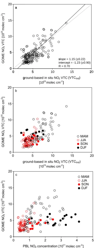
Figure 4a shows the scatter plot for the first comparison be-tween V T CGOME and V T Cind. A weighted orthogonal

re-gression is used instead of a simple linear rere-gression, because both data sets are affected by errors (York, 1966). GOME NO2 VTCs 1-sigma errors are taken from the TEMIS data

file where, for each individual pixel, an error estimate is given (Boersma et al., 2004). The error assessment for each of the ground-based VTCs follows Sect. 3.1.4. Interestingly, the independently calculated error estimates for the two data sets are very similar: the mean GOME 1-sigma error and the mean ground-based VTC error are determined to be 56% and 49%, respectively. The slope and the intercept (with their standard deviations) are calculated to be 1.15 (±0.22) and −1.23 (±0.90), respectively, with a correlation coeffi-cient R=0.70. Although there is a good general agreement between the two column data sets, the regression indicates a tendency of small GOME columns slightly underestimat-ing the correspondunderestimat-ing ground-based columns. This is further discussed in Sect. 4.3.2.

The seasonal behaviour is very similar (Fig. 4b). The small summertime NO2 VTCs mirror the shorter chemical

lifetime of NO2during photochemically active summer days

(Spicer, 1982; Warneck, 2000). Furthermore, both column data sets independently detect the largest NO2 VTCs

dur-ing the sprdur-ing season. Moxim et al. (1996) simulated the global tropospheric chemistry of peroxyacetyl nitrate (PAN) and NOxand found regional NOxspring maxima in the lower

troposphere of the northern hemisphere. This is consistent with Penkett and Brice (1986) who suggested the measured PAN maximum in spring to be due to the accumulation of precursor substances (such as NOx) during the cold

sea-son and subsequent photochemistry in spring leading to en-hanced photooxidants such as PAN and ozone. Note, how-ever, that the latter studies focused on a larger region than middle Europe. Nevertheless, due to their vertical extension, the GOME columns investigated here could be affected by

air masses representative for a larger spatial scale similarly to elevated measurement sites in the Alpine region. At such sites, the NO2concentration also shows a spring maximum

(Staehelin et al., 2000; BUWAL, 2004). The good agreement for the spring NO2 VTCs can be seen as a crude validation

of both NO2column data sets.

The qualitative comparison between the GOME NO2

VTCs and the PBL NO2 concentrations (derived following

Sect. 3.1.1, Fig. 4c) shows that a proper comparison requires information on the vertical NO2 distribution. As expected,

the near-ground NO2 concentrations are highest in winter,

mainly due to near-ground inversions that often occur during this season. In summer, the near-ground NO2concentrations

are lowest because of stronger photochemical activity and vertical mixing leading to dilution. The NO2 VTC spring

maximum is not mirrored in the average PBL NO2

concen-tration.

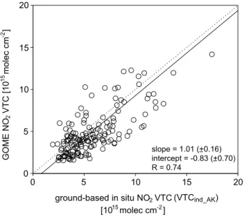
4.2.2 Second comparison

The second comparison is shown in Fig. 5. Again, a weighted orthogonal regression is calculated based on both the GOME NO2 VTC 1-sigma errors and the ground-based NO2VTC

errors estimated following Sect. 3.1.4. The mean errors for both data sets are again similar, with a mean GOME 1-sigma error of 48% and a mean error for the ground-based VTCs of 45%. The resulting slope and intercept (with their stan-dard deviations) are calculated to be 1.01 (±0.16) and −0.83 (±0.70), respectively, with a correlation coefficient R=0.74. The inclusion of AK information tends to improve the com-parison. Nevertheless, the offset still gives evidence for small GOME columns slightly underestimating the corresponding ground-based columns.

It should, however, be noted that the orthogonal regres-sion depends on the errors attributed to the data sets. These errors are estimates that also have their uncertainties. Tests performed with varying errors indicated somewhat changing results for slopes and offsets. However, independent from changes in the errors, the slopes of the orthogonal regression together with their standard deviations indicate, that the mul-tiplication with the AK has a relatively weak impact. This is due to – on average – similar shapes of the a priori and the ground-based NO2profiles. Thus, the a priori profile shapes

calculated with the CTM reproduce the tropospheric NO2

distribution seen from the ground-based measurements well for clear sky cases. This can also be seen in the scatter plot between V T Cindand V T Cind AK(Fig. 6). Although the

lat-ter is slightly higher, the relatively small difference between the two columns can be attributed to the small difference in the two NO2profile shapes (it will be shown that this

differ-ence is much larger for cloudy cases). Martin et al. (2004) similarly found a good agreement between CTM NO2

pro-files and profile information from aircraft campaigns, al-though a different model was used to generate a priori profile shapes for the retrieval.

0 è 5 é 10 15 20 a ê G O M E N O2 V T C [ 1 0 1 5 m o le c c m -2] 0 è 5 é 10 15 ë2 0 g ì round-based in situ NO2 VTC [1015 _{molec cm}-2_]í (VTCind) s î lope = 1.15 (+0.22) R = 0.70 intercept = -1.23 (+0.90)- -0 ï 5 ð 10 15 20 G O M E N O2 V T C [ 1 0 1 5 m o le c c m -2] 0 ï 5 ð 10 15 ñ2 0 g ò round-based in situ NO2 VTC [1015 molec cm-2] ó (VTCind) b ô MAM DJF S õ ON J ö JA 0 ÷ 5 ø 10 15 20 G O M E N O2 V T C [ 1 0 1 5 m o le c c m -2] 0 ÷ 1 2 ù3 4 PBL NO concentration2 [1011 molec cm-3] ú 5 ø c û MAM DJF S ü ON J ý JA

Fig. 4. Clear sky first comparison between GOME NO• and the (directly integrated) ground-based NO• VTCs

including orthogonal regression output (a). The same comparison showing the four seasons MAM, JJA, SON and DJF (b). Qualitative comparison between GOME NO• VTCs and PBL NO• concentrations (c).

37

Fig. 4. Clear sky first comparison between GOME NO2 and the

(directly integrated) ground-based NO2VTCs including

orthogo-nal regression output (a). The same comparison showing the four seasons MAM, JJA, SON and DJF (b). Qualitative comparison be-tween GOME NO₂VTCs and PBL NO₂concentrations (c).

0 5 10 15 20 GOME NO 2 VTC [10 15 molec cm -2 ] 0 5 10 15 20 ground-based in situ NO2 VTC [1015 _{molec cm}-2_] (VTCind_AK) slope = 1.01 (+0.16) R = 0.74 intercept = -0.83 (+0.70)-

-Fig. 5. Clear sky comparisons between GOME NO2VTCs and

ground-based NO₂columns with orthogonal regression output for the second comparison (ground-based profiles multiplied with the AK).

4.3 Quantifying differences between the NO2VTCs

In this section, relative differences between the two column data sets are analysed in more detail. The errors in both the GOME and the ground-based NO2 columns are not taken

into account. First, for the whole data set, the mean and median relative difference with respect to the ground-based columns (10), as well as the mean absolute difference

be-tween the columns is compared to results from other studies. This is followed by a detailed analysis of relative differences with respect to the GOME columns (11−3, Sect. 3.2.2).

4.3.1 VTC differences relative to ground-based NO2VTCs

For the whole clear sky column data set, the mean, stan-dard deviation and median of 10are calculated to be −7%,

40% and −13% (Table 4). The standard deviation sug-gests that the a priori estimates of 50% errors on clear sky GOME and ground-based columns are too conserva-tive, and errors of the order of 30% would be more con-sistent with the intercomparison results. The mean 10

in-dicates that on average, the GOME NO2 VTCs are slightly

smaller than the corresponding ground-based columns. This result is consistent with findings from other authors (Ta-ble 1) that found GOME columns being smaller than in-dependently measured columns by 14% (Petritoli et al., 2004), 8% (Martin et al., 2004) and 3% (Heland et al., 2001). The mean and median absolute difference between GOME and the directly integrated ground-based columns (V T Cind)are 0.51×1015molec cm−2(with a standard

devi-ation of 1.9×1015molec cm−2)and 0.66×1015molec cm−2,

slope = 1.17 (+0.17) R = 0.93 0 5 10 15 20 NO2 VTCind [1015 molec cm-2] 0 5 10 15 20 -intercept = -0.40 (+0.72) -NO 2 VTC ind_AK [10 15 molec cm -2]

Fig. 6. Clear sky comparison between the directly integrated ground-based NO2 column (V T Cind)and the corresponding

col-umn after multiplication with the AK (V T Cind AK). Additionally,

the resulting orthogonal regression calculation is shown.

which is comparable to the mean absolute difference of 0.49×1015molec cm−2 reported by Martin et al. (2004). Note, however, that there are also considerable differences between the Bremen, Harvard and KNMI/BIRA retrievals (van Noije et al., 2006).

4.3.2 VTC differences relative to GOME NO2VTCs:

de-tailed analysis

Unlike 10, 11−3are relative differences calculated with

re-spect to the GOME columns. These differences allow split-ting the total relative difference (11)into two contributions, – 12, which is due to errors in the ground-based NO2

pro-file, retrieval errors such as the estimate of the strato-spheric background and/or the scattering weights ml (including estimated forward model parameters such as, e.g., surface albedo),

– 13, which depends on differences between the shapes

of the a priori and the ground-based NO2profiles.

The mean, standard deviation and median of 11−3are

calcu-lated for the whole clear sky data set (157 cases) as well as for 3 subclasses equally proportioned: GOME NO2VTC<3.5,

3.5–5.0 and >5.0×1015molec cm−2_{(Table 4). In the}

fol-lowing, we allude to the means, because this allows to write 11as the sum of 12and 13.

For the whole clear sky data set, the mean 11−3 are

cal-culated to be −26%, −34% and 8%, respectively. As 10

before, 11indicates an underestimation of GOME with

re-spect to the ground-based columns. The mean 12dominates

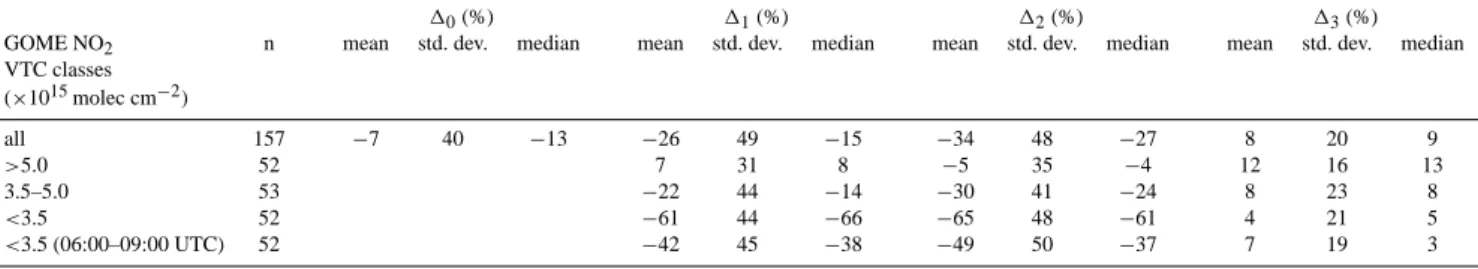
Table 4. Mean, standard deviation and median of the relative differences 10and 11−3between GOME and ground-based NO2VTCs. 10

is the relative difference calculated with respect to the ground-based columns and is, therefore, comparable to the quantities given in Table 1.

11−3are calculated with respect to the GOME columns. This allows to split the total relative difference (11)into two contributions: one

that is due to differences in the shapes of the a priori and the ground-based NO2profile (13), and another that is due to the remaining retrieval

parameters and uncertainties in the ground-based profile (12). For the subclass with GOME NO2VTCs<3.5×1015molec cm−2a second

scenario is calculated with ground-based NO2columns deduced from ground-based in situ measurements averaged from 06:00–09:00 UTC

(instead of 09:00–12:00 UTC).

1₀(%) 1₁(%) 1₂(%) 1₃(%)

GOME NO2 n mean std. dev. median mean std. dev. median mean std. dev. median mean std. dev. median VTC classes (×1015molec cm−2) all 157 −7 40 −13 −26 49 −15 −34 48 −27 8 20 9 >5.0 52 7 31 8 −5 35 −4 12 16 13 3.5–5.0 53 −22 44 −14 −30 41 −24 8 23 8 <3.5 52 −61 44 −66 −65 48 −61 4 21 5 <3.5 (06:00–09:00 UTC) 52 −42 45 −38 −49 50 −37 7 19 3

to a certain extent. As 12 is independent of a priori

pro-file errors in the retrieval, the large contribution indicates that the ground-based NO2 profiles together with the

scat-tering weights are, on average, higher than SCDtrop. The

small contribution from 13on the total 11can be attributed

to similar shapes of the a priori and the ground-based NO2

profiles. This is consistent with the relatively weak impact after inclusion of AK information as discussed in the previ-ous section. The positive value of 13indicates that the TM4

a priori NO2profile shapes are, on average, slightly biased

towards higher NO2abundances at lower altitudes or smaller

NO2abundances at higher altitudes. I.e., TM4 profiles tend

to peak more towards the surface than the observed profiles.

For the subclass with GOME NO2

VTCs>5.0×1015molec cm−2_{, the mean 1}

1−3 are

cal-culated to be 7%, −5% and 12%, respectively. Thus, for this data subset, the positive 11 is consistent with GOME

columns that are on average exceeding the ground-based columns. This explains the steeper slope for the first comparison (Fig. 4a). The small 12of −5% indicates that

the ground-based NO2profiles together with the scattering

weights reliably reproduce SCDtrop. The remaining 13

of 12% shows that differences in the two NO2 profile

shapes play a major role for this data subset. Therefore, the multiplication of the ground-based profiles with the AK has a larger impact in this data subset and explains to large parts the changing slope between the first and the second comparison (Figs. 4a and 5). The positive value again indicates TM4 a priori NO2 profile shapes that are,

on average, biased towards higher NO2abundances at lower

altitudes or smaller NO2abundances at higher altitudes. The

reasons for that are manifold and could be uncertainties in the NOx emission inventories, uncertainties arising from

the CTM, uncertainties in the meteorological fields (e.g. an underestimation of vertical transport in the alpine region), but also errors in the ground-based NO2profile. Which of

the uncertainties is dominant is not clear.

For the subclasses with GOME NO2VTCs between 3.5

and 5.0×1015molec cm−2 and <3.5×1015molec cm−2, 11−3are calculated to be −22%, −30% and 8% and −61%,

−65% and 4%, respectively (Table 4). Thus, for lower GOME NO2column values,

– 11is increasing with GOME columns underestimating

the ground-based columns,

– 12is increasing as well, indicating that SCDtrop

under-estimates the slant column given by the ground-based profile together with the scattering weights,

– the profile shapes are more similar than for situations with high GOME NO2column values.

The increasing 11 towards smaller GOME columns is

mainly explained by 12. This is the main reason for the

off-sets found in the orthogonal regression calculations (Figs. 4a and 5). Therefore, 11can no longer be explained by

differ-ent NO2profile shapes, but by uncertainties in the

ground-based NO2profiles, retrieval errors such as the estimate of

the stratospheric background and/or the scattering weights. Smaller NO2 columns in both data sets often occur in

the summer season (Fig. 4b). Therefore, one might argue that the increase in 12 towards smaller columns is mainly

due to thermal upslope transport of NO2that leads to a

sys-tematic overestimation of the NO2 located at elevated

lev-els in the ground-based profiles. To check this, we changed the averaging time window (for calculating the average NO2

concentration for the ground stations; see Sect. 3.1.1) from 09:00–12:00 to 06:00–09:00 UTC. For this time window, the influence from thermal upslope transport at the elevated stations can be expected to be small. For GOME NO2

VTCs<3.5×1015molec cm−2the resulting 11−3are −42%,

−49% and 7%, respectively (Table 4). Although 11and 12

now indicate a smaller relative difference between the col-umn data sets, thermal upslope transport of pollution only explains 1/3 (1/2 if the median is considered) of the relative

difference. It therefore seems likely that, towards smaller NO2 columns, GOME retrievals over the study area indeed

underestimate the true NO2 column. This would be

con-sistent with some unrealistically small GOME NO2 VTCs

that have been found (and that have been excluded from the comparison by the criterion SCDtrop/SCD, as pointed out at

the beginning of Sect. 4.2). For instance, the smallest clear sky GOME column of 0.05×1015molec cm−2was detected over an area covering the most polluted part of the Swiss Plateau including the largest Swiss cities Zurich and Basel. The total and the stratospheric SCD are very similar in this case (7.74×1015molec cm−2 and 7.71×1015molec cm−2, respectively), and uncertainty in the latter can at least par-tially explain the small GOME NO2VTC value.

The investigation described above should be refined fur-ther in the future. Particularly for cases with 12

explain-ing the major part of 11, independent knowledge of

non-profile retrieval parameters, such as surface albedo, would shed further light on the reason for column differences. The results presented here should be seen as tendencies, because averaged differences with large standard deviations are dis-cussed. This means that for single day-to-day cases, param-eters such as the a priori NO2profile shape can have a much

larger (but also lower) impact than averaged over the whole data set. Moreover, the investigated GOME pixels exhibit a large extension always detecting a somewhat changing mix of remote and polluted areas in the study area. For future work with smaller pixels from SCIAMACHY (60×30 km2) or the Ozone Monitoring Instrument (OMI, 13×24 km2), the pixel-to-pixel NO2VTC differences can be expected to be

much larger with remote and polluted pixels lying close to each other and probably being retrieved with similar or even the same a priori profile shapes (due to significant spatial un-dersampling with coarser resolved CTMs). We would there-fore expect that the tendencies found in the present study will come out clearer for satellite pixels with a lower extension.

5 Results for cloudy conditions

A detailed comparison for cloudy GOME pixels has so far not been carried out. The potential retrieval errors under cloudy conditions can, however, be thought to be much larger than for clear sky conditions. This is mainly due to inaccu-rate knowledge of cloud characteristics (e.g. cloud top height, cloud fraction, optical thickness) and difficulties in the radia-tive transfer modelling (multiple scattering). For the compar-ison under cloudy conditions the following has to be fulfilled: – GOME pixel location above northern Switzerland

(Fig. 1),

– GOME pixel cloud fraction from FRESCO (Koelemei-jer et al., 2001) ≥0.75,

– SCDtrop/SCD>10%.

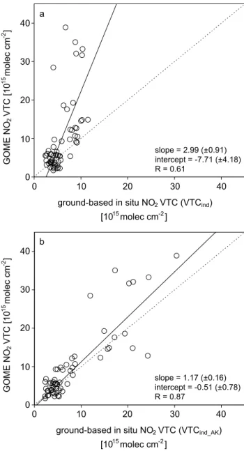
Figure 7a shows the first and the second comparison be-tween the GOME and the ground-based NO2 VTCs for 76

cloudy cases. Obviously, there are a number of cases with a very poor agreement, with GOME columns being up to a factor of 20 higher than the ground-based columns. The rea-son for the strong disagreement for these cases is discussed qualitatively at the example of the most extreme case on 17 February 2001.

Based on GOME NO2measurements, Schaub et al. (2005)

have shown that, during 16 and 17 February 2001, frontal activity over Central Europe caused vertical transport of polluted near-ground air masses to up to approximately 4000 m a.s.l. No lightning activity was detected dur-ing that episode (http://www.wetterzentrale.de/topkarten/ tkbeoblar.htm), but the vertical transport led to a significant amount of NO2being located within and above a dense cloud

cover with a top height of approximately 700 hPa. Because of the high sensitivity of the space-borne instrument above reflecting clouds, this is consistent with a large SCDtrop of

57×1015molec cm−2(which is nearly 90% of the total SCD of 64×1015molec cm−2)given by the KNMI/BIRA data set. From this, an unrealistically high GOME NO2VTC value of

489.5×1015molec cm−2is retrieved.

The corresponding ground-based NO2 VTCs are

calcu-lated to be 22.4×1015molec cm−2(directly integrated) and 38.3×1015molec cm−2(AK included). The strong disagree-ment between the latter and the GOME column indicates that the ground-based profile together with the scattering weights is much smaller than SCDtrop. Thus, two main reasons could

explain the strong disagreement: on the one hand, the scat-tering weights could be wrong due to errors in the radiative transfer modelling resulting from uncertainties in the cloud parameters. It has been mentioned in Sect. 2.1 that errors induced by uncertainties in the cloud top height are increas-ing for situations with enhanced NO2concentrations close to

the cloud top height (which is the case here). On the other hand, the disagreement can just as well be attributed to the ground-based profile: first, no NO2measurements from the

high-alpine site Jungfraujoch are available for this episode (such data gaps can be neglected when calculating a clear sky column with typically very low NO2 concentrations at

Jungfraujoch; however, they become important when pol-luted air masses reach the station and the latter additionally being located above a reflecting cloud cover). Second, the peak NO2 concentrations measured at the ground stations

occurred rather in the evening of the 17 February, and not during the time of the GOME overpass. This shows that the assumption of a homogeneous NO2distribution at elevated

levels may not be valid for this case.

Therefore, a new scenario is calculated based on the following assumptions: a) the Jungfraujoch station mea-sures the same NO2 concentration as the Zugspitze

sta-tion, and b) every ground station contributes to the ground-based column with its maximum NO2 concentration

0 100 200 300 400 GOME NO 2 VTC [10 15 molec cm -2 ] 0 10 20 30 40

ground-based in situ NO2 VTC [1015 molec cm-2]

50 500 600 direct comparison AK comparison a -500 0 500 1000 1500 2000 2500 SCDtrop/SCD 100 [%] (VTC GOME -VTC ind )/VTC ind 100 [%] 0 20 40 60 80 100 x x b

Fig. 7. First and second comparison for cloudy conditions (note the

unrealistically high columns that can be retrieved under such con-ditions) (a). Relative difference (10)between GOME and

ground-based NO₂VTCs (V T C_ind)as a function of fraction of SCDtrop

on the total SCD (b).

half of 18 February). This yields ground-based columns of 46.7×1015molec cm−2 (directly integrated, V T Cind) and

304.8×1015molec cm−2 after multiplication with the AK (V T Cind AK).

V T Cind still strongly underestimates the GOME NO2

VTC, although the lower ground stations contributed with high concentrations in the order of 30 ppb to the column. Remarkably, for this new scenario, V T Cind AK results in a

value that is at least of the same order as the GOME col-umn of 489.5×1015molec cm−2. The distinct change in the ground-based columns after multiplication with the AK in-dicates that the shapes of the ground-based and the a pri-ori NO2 profile are strongly differing. The increase of the

column after multiplication with the AK is consistent with

slope = 2.99 (+0.91) R = 0.61 0 20 30 40 GOME NO 2 VTC [10 15 molec cm -2 ]

ground-based in situ NO2 VTC (VTCind)

[1015 _{molec cm}-2_] 0 10 20 30 40 -intercept = -7.71 (+4.18) -10 a slope = 1.17 (+0.16) R = 0.87 0 20 30 40 GOME NO 2 VTC [10 15 molec cm -2 ]

ground-based in situ NO2 VTC (VTCind_AK)

[1015 _{molec cm}-2_] 0 10 20 30 40 -intercept = -0.51 (+0.78) -10 b

Fig. 8. First comparison between GOME NO2 VTCs and

tro-pospheric columns derived from ground-based in situ measure-ments (a) and second comparison after multiplying the ground-based profile with the averaging kernel (b) together with or-thogonal regression output for cloudy conditions. Columns with

SCDtrop/SCD>50% are rejected.

a TM4 a priori NO2 profile shape that is biased towards

higher NO2 abundances at lower altitudes or smaller NO2

abundances at higher altitudes. The latter point gives evi-dence for the following additional explanation of the large GOME column during this episode (besides uncertain cloud parameters): the frontal transport event results in complex air mass mixing together with horizontal and vertical movement which may not be properly reproduced by the coarsely re-solved global CTM. The CTM might therefore calculate an a priori NO2 profile that underestimates the enhanced NO2