HAL Id: hal-00414722
https://hal.archives-ouvertes.fr/hal-00414722
Submitted on 8 Jan 2016
HAL is a multi-disciplinary open access
archive for the deposit and dissemination of
sci-entific research documents, whether they are
pub-lished or not. The documents may come from
teaching and research institutions in France or
abroad, or from public or private research centers.
L’archive ouverte pluridisciplinaire HAL, est
destinée au dépôt et à la diffusion de documents
scientifiques de niveau recherche, publiés ou non,
émanant des établissements d’enseignement et de
recherche français ou étrangers, des laboratoires
publics ou privés.
IASI: comparison with correlative satellite,
ground-based and ozonesonde observations
Anne Boynard, Cathy Clerbaux, Pierre-François Coheur, Daniel Hurtmans,
Solène Turquety, Maya George, Juliette Hadji-Lazaro, C. Keim, J.
Meyer-Arnek
To cite this version:
Anne Boynard, Cathy Clerbaux, Pierre-François Coheur, Daniel Hurtmans, Solène Turquety, et al..
Measurements of total and tropospheric ozone from IASI: comparison with correlative satellite,
ground-based and ozonesonde observations. Atmospheric Chemistry and Physics, European Geosciences
Union, 2009, 9 (16), pp.6255-6271. �10.5194/acp-9-6255-2009�. �hal-00414722�
www.atmos-chem-phys.net/9/6255/2009/ © Author(s) 2009. This work is distributed under the Creative Commons Attribution 3.0 License.
Chemistry
and Physics
Measurements of total and tropospheric ozone from IASI:
comparison with correlative satellite, ground-based
and ozonesonde observations
A. Boynard1,2, C. Clerbaux1, P.-F. Coheur3, D. Hurtmans3, S. Turquety1,*, M. George1, J. Hadji-Lazaro1, C. Keim2, and J. Meyer-Arnek4
1UPMC Univ. Paris 06; Universit´e Versailles St-Quentin; CNRS/INSU, LATMOS-IPSL, Paris, France
2Universit´e Paris 12 et 7; CNRS/INSU, Laboratoire Interuniversitaire des Syst`emes Atmosph´eriques-IPSL, Cr´eteil, France 3Spectroscopie de l’Atmosph`ere, Chimie quantique et Photophysique, Universit´e Libre de Bruxelles (U.L.B.),
Brussels, Belgium
4German Aerospace Center (DLR), German Remote Sensing Data Center (DFD), Oberpfaffenhofen, Wessling, Germany *now at: UPMC Univ. Paris 06; CNRS/INSU, Laboratoire de M´et´eorologie Dynamique-IPSL, Paris, France
Received: 24 February 2009 – Published in Atmos. Chem. Phys. Discuss.: 30 April 2009 Revised: 21 July 2009 – Accepted: 28 July 2009 – Published: 31 August 2009
Abstract. In this paper, we present measurements of
to-tal and tropospheric ozone, retrieved from infrared radi-ance spectra recorded by the Infrared Atmospheric Sound-ing Interferometer (IASI), which was launched on board the MetOp-A European satellite in October 2006. We com-pare IASI total ozone columns to Global Ozone Moni-toring Experiment-2 (GOME-2) observations and ground-based measurements from the Dobson and Brewer network for one full year of observations (2008). The IASI total ozone columns are shown to be in good agreement with both GOME-2 and ground-based data, with correlation co-efficients of about 0.9 and 0.85, respectively. On average, IASI ozone retrievals exhibit a positive bias of about 9 DU (3.3%) compared to both GOME-2 and ground-based mea-surements. In addition to total ozone columns, the good spec-tral resolution of IASI enables the retrieval of tropospheric ozone concentrations. Comparisons of IASI tropospheric columns to 490 collocated ozone soundings available from several stations around the globe have been performed for the period of June 2007–August 2008. IASI tropospheric ozone columns compare well with sonde observations, with corre-lation coefficients of 0.95 and 0.77 for the [surface–6 km] and [surface–12 km] partial columns, respectively. IASI re-trievals tend to overestimate the tropospheric ozone columns in comparison with ozonesonde measurements. Positive
Correspondence to: A. Boynard
average biases of 0.15 DU (1.2%) and 3 DU (11%) are found for the [surface–6 km] and for the [surface–12 km] partial columns respectively.
1 Introduction
Global monitoring of ozone (O3) is essential since this
molecule plays a key role in the photo-chemical equilibrium of the atmosphere. In the stratosphere, the ozone layer has a beneficial role as it absorbs harmful ultraviolet radiation. In contrast, ozone in the troposphere is considered by air quality agencies as one of the main air pollutants with sig-nificant impacts on human health and ecosystems. In addi-tion, ozone is one of the main greenhouse gases and plays a major role in determining the oxidizing capacity of the tro-posphere. For all these reasons, ozone needs to be moni-tored with good spatial and temporal coverage in order to better understand its evolution and its impact on air quality and climate. The measurement of tropospheric ozone is best performed by ozonesondes, which provide vertical profiles from the surface to about 30–35 km, with a very high verti-cal resolution (∼100 m) and an accuracy of about ±(5–10%) (Thompson et al., 2003a, 2007; Smit et al., 2007). Sound-ings are performed at different locations around the globe, collected mainly in the Northern Hemisphere by the World Ozone and Ultraviolet Data Centre (WOUDC). The South-ern Hemisphere Additional Ozonesondes (SHADOZ) pro-vide additional soundings in the southern and tropical regions
Fig. 1. Clear-sky IASI radiance spectra around the intense ozone
absorption band at 9.6 µm recorded at Hilo (Hawaii) in USA (red), Madrid in Spain (blue) and Summit in Greenland (black). Spec-tra are characterized by surface temperatures of 299.5, 287.1 and 255.5 K respectively.
(Thompson et al., 2003a, b, 2004, 2007), which improve the spatial coverage of the ozonesonde network. However, the coverage remains sparse and confounds attempts to gener-ate a complete global picture of tropospheric ozone concen-trations. Despite the difficulty to separate the tropospheric ozone component from the large stratospheric contribution, satellite measurements are a good way to compliment the ozonesonde observations.
The first distributions of tropospheric ozone were obtained from ultraviolet-visible (UV-vis) measurements of the Total Ozone Measurement Spectrometer (TOMS) by subtracting stratospheric ozone from total ozone (Fishman and Larsen, 1987; Fishman et al., 1990). Subsequently, several different residual-based methods have been developed to derive tropo-spheric ozone column from TOMS measurements (Ziemke et al., 1998; Thompson et al., 1999; Chandra et al., 2003). More recently, various approaches have been used to directly re-trieve ozone profiles (and thus to derive tropospheric ozone) from the Global Ozone Monitoring Experiment (GOME) measurements (Hoogen et al., 1999; Liu et al., 2005). UV-vis instruments remain by nature, however, weakly sensitive to the tropospheric ozone content.
Space-borne nadir-viewing instruments using the thermal infrared (TIR) spectral range to probe the troposphere offer maximum sensitivity in this layer with a vertical resolution of about 6 km (Coheur et al., 2005; Worden et al., 2007). The first distributions of total and tropospheric ozone have been retrieved from the Interferometric Monitor Greenhouse gases (IMG) instrument (Turquety et al., 2002, 2004; Coheur et al., 2005). However, the instrument was in operation for only 10 months in 1996 on board the Japanese ADEOS platform.
There are currently three nadir viewing TIR instruments pro-viding ozone measurements from polar-orbiting satellites: the Atmospheric InfraRed Sounder (AIRS) on AQUA, the Tropospheric Emission Spectrometer (TES) on AURA and the Infrared Atmospheric Sounding Interferometer (IASI) on MetOp-A. Extended analyses, using TES and AIRS in partic-ular have highlighted seasonal trends (Divakarla et al., 2008), enhanced pollution patterns and long-range transport (Zhang et al., 2006; Jourdain et al., 2007; Parrington et al., 2008). More recently, the enhanced capabilities of TIR sounders to probe tropospheric ozone have been used to perform an anal-ysis of the photochemical pollution events that occurred dur-ing the 2007 summer heat wave in southern Europe, with the recently launched IASI sounder (Eremenko et al., 2008). The latter study is a first step towards the use of infrared satellite observations to monitor tropospheric ozone and to improve the forecasts of air quality and climate models.
In this paper, we present the first global distributions of IASI total ozone columns, as well as IASI tropospheric ozone measured around several ozonesonde stations. The next section provides a description of the IASI ozone mea-surements, including the characteristics of the instrument and the different ozone products, such as total columns and ver-tical profiles. In Sect. 3, the IASI total and tropospheric ozone columns are compared with correlative ozone mea-surements, obtained by the GOME-2 instrument also on board the MetOp-A platform, ground-based and ozonesonde data. Section 4 summarizes the study and gives some out-looks.
2 IASI ozone measurements 2.1 IASI data
The IASI instrument (Clerbaux et al., 2007, 2009) is de-signed to measure temperature and moisture profiles with a very high accuracy for numerical weather prediction (Schl¨ussel et al., 2005). It also allows the monitoring of trace gases to improve our understanding of the interactions be-tween atmospheric chemistry, climate and pollution. It was launched on board the MetOp-A polar-orbiting satellite on 19 October 2006 and started to provide operational mea-surements in June 2007. IASI is a thermal infrared nadir-looking Fourier transform spectrometer that measures the Earth’s surface and the atmospheric radiation over a spectral range of 645–2760 cm−1with a 0.5 cm−1spectral resolution
(apodized). The ozone absorption band, near 9.6 µm, is pre-sented in Fig. 1 as measured at three locations, representative of tropical (Hilo -Hawaii- in USA), mid-latitude (Madrid in Spain) and polar (Summit in Greenland) regions and charac-terized by different surface temperatures.
The IASI field of view is a matrix of 2×2 circular pixels, each with a diameter footprint of 12 km at nadir. IASI mea-sures on average each location on the Earth’s surface twice
32
Figure 2
1 Fig. 2. Global distribution of total ozone columns obtained using
the NN algorithm for daytime cloud filtered IASI observations on 15 February 2008. The data are averaged over a 1◦×1◦grid. Only measurements made with a scan angle below 32◦on either side of the nadir are considered in the retrievals.
a day (at 09:30 and 21:30 local time), every 50 km at nadir, with an excellent horizontal coverage due to its polar orbit and its capability to scan across track over a swath width of 2200 km.
2.2 Ozone retrievals
Space-borne instruments record atmospheric spectra contain-ing thousands of absorption or emission lines organized into bands. In the TIR spectral range, each spectrum results mainly from the radiative interaction between the Earth’s thermal emission and the atmosphere. The absorption lines and trace gas concentrations are linked by a nonlinear func-tion of the surface characteristics (emissivity, temperature), the temperature profile at the location of the observation, the atmospheric components interfering in the same spectral range (such as other trace gases, clouds and aerosols), as well as the instrumental characteristics, including the spectral res-olution, the radiometric noise and the spectral response func-tion. To retrieve information about the atmosphere, such as surface temperature or atmospheric trace gas concentrations from the measured radiances, an inversion algorithm needs to be applied.
Since 4 June 2007, global distributions of total ozone columns are systematically retrieved, in a quasi near real time mode, from IASI Level 1 radiances distributed by Eumet-sat through the Eumetcast dissemination system, for daytime and night time measurements, using a fast neural network approach (Turquety et al., 2004). For specific cases ozone concentration profiles in the troposphere and in the strato-sphere with an associated error budget are derived using a line-by-line radiative transfer model coupled to an optimal
estimation inversion scheme (Coheur et al., 2005). Diagnos-tic variables allowing accurate comparison with other data are also provided, in particular the averaging kernel functions
A=∂ ˆ∂xx characterizing the sensitivity of the retrieved state ˆx
to the true state x. The trace of A represents the number of independent elements contained in the measurements, known as the degrees of freedom for signal (DOFS) which gives an estimation of the vertical sensitivity of the retrievals. The maximum sensitivity is given by the peak of the averaging kernels at a given altitude and the vertical resolution of the retrieved profiles can be evaluated by the full width at half maximum of the averaging kernel functions (Rodgers, 2000). Retrievals are only performed for cloud-free scenes, iden-tified using a filter based on the estimation of brightness tem-peratures around 11 and 12 µm and on their comparison with the surface temperature provided by the European Centre for Medium-Range Weather Forecasts (ECMWF) analyses. A more detailed description of the cloud filter is given in Cler-baux et al. (2009). The next two sections present a descrip-tion of the different ozone products obtained from the IASI measurements and used for the validation work presented in this paper.
2.2.1 Total ozone global distributions
Systematic retrievals of total ozone columns are performed using an algorithm based on neural network (NN) techniques (Turquety et al., 2004). The inputs of the NN are composed of clear-sky IASI spectra and of associated surface temper-ature and atmospheric tempertemper-ature profiles from ECMWF analyses. For a full description of the algorithm the reader is kindly referred to Turquety et al. (2004).
Figure 2 presents an example of total ozone column dis-tributions retrieved from IASI daytime measurements made on 15 February 2008, averaged over a constant 1◦×1◦grid. Only measurements made with a scan angle below 32◦on either side of the nadir are considered as the NN was not trained at larger scan angle values. This figure illustrates the capability of IASI to capture the spatial variability of the total ozone columns. Maximum columns are located at mid- and high latitudes and minimum columns are found in the tropics. On this day a remarkable feature of the total ozone columns located in the eastern Atlantic around [35◦N,
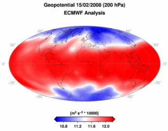
−30◦E] (see zone highlighted by the enclosed area) is ob-served by both IASI and GOME-2 (not shown). Due to a low pressure system located in the vicinity of the Canary Is-lands (see Fig. 3, which represents the geopotential height distribution at 200 hPa from the ECMWF analyses for that day) the tropopause height is massively decreased resulting in enhanced total ozone columns.
33
Figure 3
1 Fig. 3. Global distribution of the geopotential height at 200 hPa ob-tained from the ECMWF operational analyses on 15 February 2008 showing a low pressure system over the Canary Islands around [35◦N,–30◦E].
2.2.2 Ozone vertical profiles
Ozone vertical profiles are retrieved for specific areas, us-ing a radiative transfer and retrieval software (Atmosphit) based on the Optimal Estimation Method (OEM) (Rodgers, 1976, 2000). This software also provides a full characteri-zation of the retrievals in terms of vertical sensitivity and er-ror sources, which is essential for an optimal use of satellite data. A detailed description of the method and the software can be found in Coheur et al. (2005), Wespes et al. (2007) and Clarisse et al. (2008).
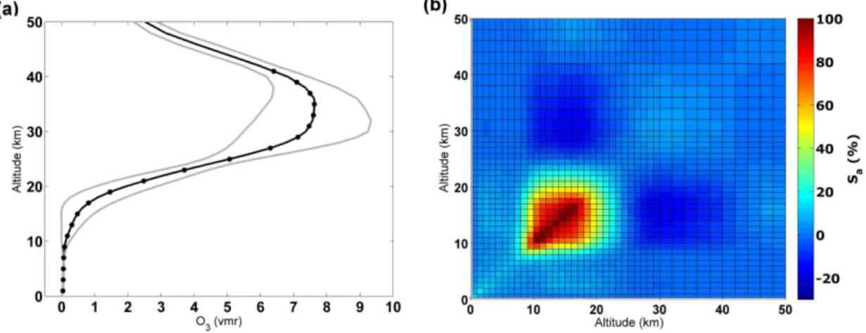
As the retrieval of ozone profiles from atmospheric spec-tra is an ill-posed problem, one needs to consspec-train the inver-sion by additional information based on the variables being retrieved. In the OEM, this constraint consists of a priori information, which is composed of an a priori mean pro-file (xa) and its associated variance-covariance matrix (Sa). These represent our knowledge of the state vector (vertical profile of ozone in our case) and its expected variability at the time and the place of the measurements. The ozone a priori profile and covariance matrix used in this work, dis-played in Fig. 4a and b respectively, are derived from a set of radiosonde measurements from all over the globe (available data during the period 2004–2008) connected to the UGAMP monthly climatology (Li and Shine, Internal Report, 1995) above 30–35 km. It is thus representative of the global and annual ozone variability. Figure 4b shows higher variability in the upper troposphere and lower stratosphere between 8 and 22 km, and lower values in other altitude ranges. Near the surface, this prior information allows relatively low vari-ability, e.g. of 10% at surface level.
In this work, the ozone profiles are retrieved in 2 km thick layers from the surface to 42 km. Surface temperature, water
vapour (H2O) partial columns and carbon dioxide (CO2) total
columns are simultaneously adjusted. The pressure and the temperature profiles are extracted from the ECMWF analy-ses and are collocated with the IASI measurements.
The most useful window to measure ozone in the TIR is around 9.6 µm, where ozone lines strongly dominate the 980–1070 cm−1 range. Ozone retrievals are performed in the 1025–1075 cm−1spectral range, in order to minimize the computation time and avoid interferences with water vapour lines. This reduced window was shown to contain all the available information for retrieving ozone profiles from ther-mal radiance. The spectroscopic parameters have been ex-tracted from the HITRAN 2004 database (Rothman et al., 2005).
The measurement covariance matrix including not only the instrumental noise but also other error sources such as the uncertainties on the temperature profiles is assumed to be diagonal with each diagonal element identical and equal to σe. The IASI radiometric noise has been estimated at 20 nW/(cm2sr cm−1) in the ozone retrieval spectral range (Clerbaux et al., 2009). We have no estimation for the other error sources. Optimization tests have been made to find the optimal value of σe. They have shown that the root mean square (RMS) of the spectral residuals (differ-ence between the measured and the calculated spectra at the last fitting iteration) at different places and times was con-tained between 17 and 200 nW/(cm2sr cm−1). A conserva-tive value σe=70 nW/(cm2sr cm−1), of about three times the radiometric noise, was selected for the retrievals on that ba-sis. Although it might reduce the extent of information avail-able in some cases, this conservative approach allows the study of ozone distributions at all latitudes and seasons us-ing the same a priori xaand Sainformation. A summary of the main retrieval settings is given in Table 1.
Figure 5 presents an example of a spectral fit and of the associated retrieved ozone profile for a case with a high total ozone column above the eastern Atlantic area identified on Fig. 2. For that case, the retrieval provides low RMS values (see residual in Fig. 5a) and the retrieval constraint was there-fore relaxed to a value of 20 nW/(cm2sr cm−1) close to the instrumental noise in order to fully exploit the available infor-mation on the vertical ozone distribution. The vertical pro-file for this particular observation is characterized by a sec-ondary ozone maximum with ozone concentrations of up to 6×10¹²molecules cm−3at about 11 km altitude. This is con-sistent with the low pressure system shown in Fig. 3 which is likely to be responsible for the transport of stratospheric (ozone enriched) air masses into the tropopause region. Po-tential vorticity, which is a tracer of stratospheric air that is transported into the troposphere, was also examined, and cor-roborates our interpretation of the stratospheric intrusion.
Figure 6a presents the averaging kernel functions for this specific observation. The averaging kernels are given for 6 km thick partial columns, from the surface to 24 km. The IASI sensitivity to the ozone profile is maximal in the
34
Figure 4
1
Fig. 4. (a) Global ozone a priori profile (black line) with its variability (grey lines, square root of the diagonal elements of the ozone a priori
variance-covariance matrix) and the retrieval levels in black dots. (b) Global ozone a priori variance-covariance matrix (Sa) in percent built from radiosonde measurements for the period 2004–2008.
35
Figure 5
1
Fig. 5. (a) Spectral fit and residual for a IASI measurement made on 15 February 2008 in the eastern Atlantic (34.8◦N,–29.3◦E); the black lines at ±20 nW/(cm2sr cm−1) correspond to the IASI radiometric noise value used to constrain this retrieval. (b) Associated retrieved (red) and a priori (black) ozone profiles in number density units.
troposphere ([surface–12 km] column), but does not allow the separation of the two independent tropospheric compo-nents for this remote case above the ocean. This measure-ment, corresponding to a surface temperature of 291.4 K is characterized by a DOFS value of 3.5, which indicates that two additional columns in the upper troposphere and lower stratosphere can be retrieved independently from the tropo-spheric column. The thermal contrast (difference between the surface temperature and the temperature of the first at-mospheric vertical layer) was calculated, and a value of 2.4 K was found, which is relatively unfavourable for tropospheric sounding in the TIR. Better information in the lower tropo-sphere is expected in the case of high positive thermal con-trast which interestingly accompanies frequent photochemi-cal pollution events (Eremenko et al., 2008). As emphasized in other papers (Deeter et al., 2007; Clerbaux et al., 2009)
DOFS numbers depend on both surface temperature and ther-mal contrast which in turn depend on surface type.
The associated error budget in Fig. 6b highlights the dom-inance of the smoothing error to the budget, with the mea-surement error and the errors introduced by the uncertainties on the temperature profile also contributing to some extent. Error sources due to the simultaneous retrievals of surface properties (temperature and emissivity) and constituent con-centrations such as H2O and CO2contribute weakly and are
not shown. The total error varies from 25 to 50% for each in-dividually retrieved level of the profile. The errors are maxi-mum around 10–15 km due to the tropopause variability. At all altitudes between 2 and 25 km however, there is an impor-tant reduction of errors compared to the a priori variability, showing the extent of information provided by the measure-ments.
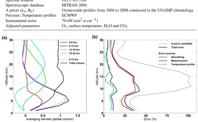
Table 1. Summary of the retrieval settings.
Spectral window 1025–1075 cm−1 Spectroscopic database HITRAN 2004
A priori (xa, Sa) Ozonesonde profiles from 2004 to 2008 connected to the UGAMP climatology Pressure, Temperature profiles ECMWF
Instrumental noise 70 nW/(cm2sr cm−1)
Adjusted parameters O3, surface temperature, H2O and CO2
36
Figure 6
1
Fig. 6. (a) Averaging kernel functions for the [surface–6], [6–12], [12–18], and [18–24] km partial columns characterizing the retrieval
shown in Fig. 4. The averaging kernel associated with the [surface–12] km tropospheric column is also shown. The black curve represents the integrated measurement response. (b) Associated error budget. The a priori variability and total errors are given by the square root of the diagonal elements of the a priori covariance matrix and the error covariance matrix, respectively. The contributions of the surface properties (surface temperature and emissivity), H2O and CO2columns are not shown.
3 Validation with available data 3.1 Total ozone
IASI total ozone column validation was performed using two sets of data: satellite data from the GOME-2 instrument and ground-based data from the Dobson and Brewer network.
3.1.1 Comparisons with GOME-2 measurements
The GOME-2 instrument, also placed aboard the MetOp-A platform is designed to continuously monitor the abundance, distribution and variability of ozone and associated species. GOME-2 is a UV-vis cross-track nadir viewing spectrometer covering the range from 240 to 790 nm. Its field of view may be varied in size from 5 km×40 km to 80 km×40 km (default). The maximum swath is about 1920 km providing almost daily global coverage at the equator.
The retrievals of total ozone columns from GOME-2 mea-surements are based on the GOME Data Processor (GDP) operational algorithm which is a classical DOAS-AMF fitting algorithm. More details on the algorithm can be found in Van Roozendael et al. (2006).
GOME-2 total ozone columns provided by the DLR are available in near real time since the 30 March 2007, through Eumetcast. A initial validation with one full year of ground-based and satellite measurements shows that GOME-2 to-tal ozone products have already reached an excellent quality (Balis et al., Validation report, 2008, can be obtained from: http://wdc.dlr.de/sensors/gome2/).
For the validation of IASI total ozone column retrievals, IASI and GOME-2 total ozone column distributions were av-eraged over a constant 1◦×1◦ grid and compared over the whole year of 2008. As the UV-vis instrument provides day-time observations, only the IASI dayday-time measurements are compared. Figure 7 shows the seasonal global distributions of total ozone columns derived from the IASI NN retrievals compared to the GOME-2 data. Globally and seasonally both instruments observe similar structures for the total ozone columns as a function of latitude. As expected, maximum columns are observed at high latitudes whereas the minimum columns are generally located in the tropical regions (except for the ozone hole seasons). The annual ozone depletion over the Antarctic for the July-August-September and October-November-December periods is also well observed by both instruments.
37
Figure 7
1
Fig. 7. Global distributions for three months averaged periods (1◦×1◦grid): (left) IASI total ozone columns compared to (right) GOME-2 retrieved total ozone columns for daytime measurements. On the IASI maps, grey areas correspond to data recorded over topography (altitude higher than 2 km) that have been filtered out.
A statistical comparison has been performed between the total ozone columns retrieved from IASI and GOME-2 sep-arately for each season, at global scale and for five differ-ent latitude zones (Fig. 8). The correlation coefficidiffer-ent, the bias of the mean and the standard deviation (or RMS error)
from these comparisons are summarized in Table 2. Over the globe, the agreement between the two distributions is very good, with correlation coefficients ranging from 0.92 to 0.98 and an RMS error of 9.7 to 28.2 DU depending on the sea-sons. This comparison also highlights an overestimate of the
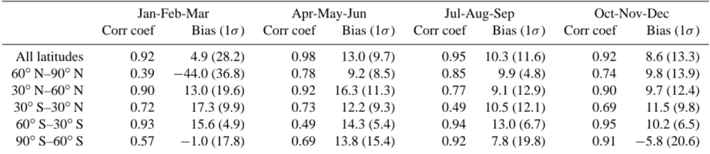
Table 2. Summary of the correlation, the bias and the (1σ ) standard deviation (RMS) of the IASI total ozone column relative to the GOME-2
data, for each season. The bias and the standard deviation are given in Dobson units.
Jan-Feb-Mar Apr-May-Jun Jul-Aug-Sep Oct-Nov-Dec Corr coef Bias (1σ ) Corr coef Bias (1σ ) Corr coef Bias (1σ ) Corr coef Bias (1σ ) All latitudes 0.92 4.9 (28.2) 0.98 13.0 (9.7) 0.95 10.3 (11.6) 0.92 8.6 (13.3) 60◦N–90◦N 0.39 −44.0 (36.8) 0.78 9.2 (8.5) 0.85 9.9 (4.8) 0.74 9.8 (13.9) 30◦N–60◦N 0.90 13.0 (19.6) 0.92 16.3 (11.3) 0.77 9.1 (12.9) 0.90 9.7 (12.4) 30◦S–30◦N 0.72 17.3 (9.9) 0.73 12.2 (9.3) 0.49 10.5 (12.1) 0.69 11.5 (9.8) 60◦S–30◦S 0.93 15.6 (4.9) 0.49 14.3 (5.4) 0.94 13.0 (6.7) 0.95 10.2 (6.5) 90◦S–60◦S 0.57 −1.0 (17.8) 0.69 13.8 (15.4) 0.92 7.8 (19.8) 0.91 −5.8 (20.6) 38 Figure 8
1 Fig. 8. Scatter plots of the IASI and GOME-2 total ozone columns
for three months averaged periods (Jan-Feb-Mar, Apr-May-Jun, Jul-Aug-Sep, Oct-Nov-Dec). The plots show averaged data over a 1◦×1◦grid. The shaded line represents the linear regressions be-tween all data points and the black line, of unity slope, is shown for reference.
IASI total ozone columns with respect to GOME-2 (positive bias ranging from 4.9 DU (2.9%) to 13 DU (4.4%)). On aver-age over the year, the bias value is around 9 DU (∼3%) which is in the same order of magnitude as that found by Osterman et al. (2008) for TES total ozone columns compared to OMI data. The detailed analysis undertaken for different latitude bands shows that the bias may be negative, e.g. at high lat-itudes. In particular, in the winter northern polar regions, comparisons between IASI and GOME-2 total ozone show the largest bias (−44.0 DU), RMS error (36.8 DU) and the lowest correlation coefficient (0.39) of all seasons. The high-est correlation coefficients are found in the mid-latitude re-gions, with values higher than 0.9, except for the summer northern and the autumn southern mid-latitude regions where
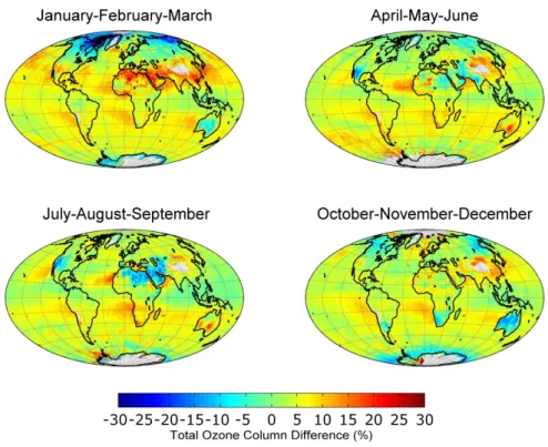
the correlation coefficients are lower. In order to examine precisely the regions characterized by larger discrepancies, relative differences between IASI and GOME-2 total ozone columns have been calculated for each season and are shown in Fig. 9. Globally relative differences do not exceed 15% and no significant latitudinal dependence is apparent. Al-though more efforts are obviously required to fully under-stand local discrepancies, it is partly attributable to the ferent observation modes. First the instruments have a dif-ferent footprint on the ground (12 km for IASI (circular), 40×80 km for GOME-2) and are hence subject to different cloud contamination. Secondly, the geometry of the obser-vation differs, which implies that different air masses are probed. Moreover, the prior information used in both re-trieval algorithms is different. Finally, the two instruments are characterized by different weighting functions and have different vertical sensitivities. GOME-2 has a maximum sen-sitivity in the stratosphere, while IASI presents a maximum sensitivity in the free troposphere. The largest differences observed at high latitudes are attributed to the low signal noise ratio recorded by the IASI instrument especially in the winter northern polar regions but also to the degradation of the GOME-2 precision at higher solar zenith angles in these regions. In the tropics, the largest differences are observed above regions characterized by extreme emissivities, such as sandy surfaces (e.g. Sahara, Middle East), that are not ac-counted for in the IASI near-real-time processing chain us-ing the NN. Another plausible source of discrepancy in these areas might come from the presence of aerosols (e.g. above western Africa for the first trimester).
3.1.2 Comparisons with ground-based measurements
The ground-based total ozone data used in this study are from Dobson and Brewer UV spectrophotometer measure-ments. Total ozone can be derived from direct sun, zenith sky or focused moon observations at different wavelengths. The Dobson instrument, originally developed in the 1920s (Dobson, 1931), uses four wavelengths (two pairs) to deter-mine total ozone quantities. The most commonly used pairs are the AD double pair (305.5/325.5 nm and 317.6/339.8 nm)
39
Figure 9
1
Fig. 9. Relative differences between IASI and GOME-2 total ozone columns for daytime measurements and for three month averaged periods
(1◦×1◦grid). The relative differences are calculated according to: 100*(IASI-GOME2)/GOME2.
Fig. 10. Total ozone columns derived from collocated IASI and
ground-based measurements with associated standard deviations, zonally averaged for 2008.
and the CD pair (311.45/332.4 nm and 317.6/339.8 nm). The Brewer spectrophotometer, available since the early eighties (Brewer, 1973) relies on the same principle as the Dobson instrument, however, the instrument uses several wavelength pairs from five wavelengths between 306.3 and 320.1 nm to derive total ozone. Both Dobson and Brewer instruments
Fig. 11. Scatter plots of the IASI and ground-based total ozone
columns for 2008. The correlation, bias, standard deviation and number of collocated observations are also indicated on the top of the figure. The shaded line represents the linear regressions be-tween all data points and the black line, of unity slope, is shown for reference. The bias (in relative value) is calculated according to: 100*(IASI-ground-based)/ground-based.
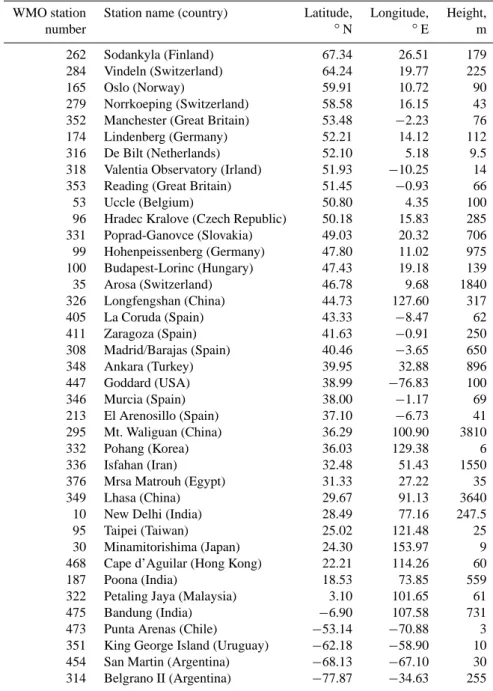
Table 3. List of Brewer stations used for the ozone validation.
WMO station Station name (country) Latitude, Longitude, Height,
number ◦N ◦E m
262 Sodankyla (Finland) 67.34 26.51 179 284 Vindeln (Switzerland) 64.24 19.77 225
165 Oslo (Norway) 59.91 10.72 90
279 Norrkoeping (Switzerland) 58.58 16.15 43 352 Manchester (Great Britain) 53.48 −2.23 76 174 Lindenberg (Germany) 52.21 14.12 112 316 De Bilt (Netherlands) 52.10 5.18 9.5 318 Valentia Observatory (Irland) 51.93 −10.25 14 353 Reading (Great Britain) 51.45 −0.93 66 53 Uccle (Belgium) 50.80 4.35 100 96 Hradec Kralove (Czech Republic) 50.18 15.83 285 331 Poprad-Ganovce (Slovakia) 49.03 20.32 706 99 Hohenpeissenberg (Germany) 47.80 11.02 975 100 Budapest-Lorinc (Hungary) 47.43 19.18 139 35 Arosa (Switzerland) 46.78 9.68 1840 326 Longfengshan (China) 44.73 127.60 317 405 La Coruda (Spain) 43.33 −8.47 62 411 Zaragoza (Spain) 41.63 −0.91 250 308 Madrid/Barajas (Spain) 40.46 −3.65 650 348 Ankara (Turkey) 39.95 32.88 896 447 Goddard (USA) 38.99 −76.83 100 346 Murcia (Spain) 38.00 −1.17 69 213 El Arenosillo (Spain) 37.10 −6.73 41 295 Mt. Waliguan (China) 36.29 100.90 3810 332 Pohang (Korea) 36.03 129.38 6 336 Isfahan (Iran) 32.48 51.43 1550 376 Mrsa Matrouh (Egypt) 31.33 27.22 35 349 Lhasa (China) 29.67 91.13 3640 10 New Delhi (India) 28.49 77.16 247.5 95 Taipei (Taiwan) 25.02 121.48 25 30 Minamitorishima (Japan) 24.30 153.97 9 468 Cape d’Aguilar (Hong Kong) 22.21 114.26 60 187 Poona (India) 18.53 73.85 559 322 Petaling Jaya (Malaysia) 3.10 101.65 61 475 Bandung (India) −6.90 107.58 731 473 Punta Arenas (Chile) −53.14 −70.88 3 351 King George Island (Uruguay) −62.18 −58.90 10 454 San Martin (Argentina) −68.13 −67.10 30 314 Belgrano II (Argentina) −77.87 −34.63 255
present similar performances (Kerr et al., 1988). The Dob-son and Brewer total ozone measurements have already been used for the validation of satellite derived total ozone mea-surements (Weber et al., 2005; Balis et al., 2007).
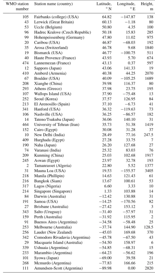
For the comparisons with IASI total ozone columns, we used all the Dobson and Brewer data derived from direct sun and zenith sky observations available for 2008 from the WOUDC archives. The data format currently used consists of daily total ozone values expressed in Dobson units. We set the coincidence criteria to 0.5◦ radius from the ground-based station and to the same day of observation. IASI measurements collocated to ground-based
measure-ments were then averaged. 39 Brewer and 50 Dobson sta-tions were considered for the comparison. The stasta-tions are summarized in Tables 3 and 4.
Figure 10 shows the collocated total ozone distributions averaged over 5◦ latitude bands for the year 2008. A pos-itive bias between the two distributions is apparent, with larger differences at mid- and low latitudes, in particular in the Southern Hemisphere. The variability associated with IASI total ozone columns is somewhat larger than that of the ground-based measurements, except at high latitudes where the latter increases.
Table 4. List of Dobson stations used for the ozone validation.
WMO station Station name (country) Latitude, Longitude, Height,
number ◦N ◦E m
105 Fairbanks (college) (USA) 64.82 −147.87 138 43 Lerwick (Great Britain) 60.13 −1.18 80 53 Uccle (Belgium) 50.80 4.35 100 96 Hadrec Kralove (Czech Republic) 50.18 15.83 285 99 Hohenpeissenberg (Germany) 47.80 11.02 975 20 Caribou (USA) 46.87 −68.03 192 35 Arosa (Switzerland) 46.78 9.68 1840 19 Bismarck (USA) 46.77 −100.75 511 40 Haute Provence (France) 43.93 5.70 674 474 Lannemezan (France) 43.13 0.37 597 12 Sapporo (Japan) 43.06 141.33 19 410 Amberd (Armenia) 40.38 44.25 2070 67 Boulder (USA) 40.09 −105.25 1689 208 Xianghe (China) 39.98 116.37 80 293 Athens (Greece) 37.98 23.75 195 107 Wallops Island (USA) 37.90 −75.48 13 252 Seoul (Korea) 37.57 126.95 84 213 El Arenosillo (Spain) 37.10 −6.73 41 341 Hanford (USA) 36.32 −119.63 73 106 Nashville (USA) 36.25 −86.57 182 14 Tateno/Tsukuba (Japan) 36.06 140.10 31 464 University of Tehran (Iran) 35.73 51.38 1419
152 Cairo (Egypt) 30.08 31.28 37
10 New Delhi (India) 28.49 77.16 247.5 409 Hurghada (Egypt) 27.28 33.75 7 190 Naha (Japan) 26.20 127.68 27 74 Varanasi (India) 25.32 83.03 76 209 Kunming (China) 25.03 102.68 1917 245 Aswan (Egypt) 23.97 32.78 193 2 Tamanrasset (Algeria) 22.80 5.52 1377 31 Mauna Loa (USA) 19.53 −155.57 3405 218 Manila (Phillipin) 14.63 121.43 61 216 Bangkok (Siam) 13.67 100.61 53 317 Lagos (Nigeria) 6.60 3.33 10 214 Singapore (Singapore) 1.33 103.88 14 84 Darwin (Australia) −12.42 130.88 31 191 Samoa (USA) −14.25 −170.56 82 27 Brisbane (Australia) −27.42 153.12 3 343 Salto (Uruguay) −31.40 −57.97 31 159 Perth (Australia) −31.92 115.95 2 91 Buenos Aires (Argentina) −34.58 −58.48 25 253 Melbourne (Australia) −37.74 144.90 128.5 256 Lauder (New Zealand) −45.03 169.68 370 342 Comodoro Rivadavia (Argentina) −45.78 −67.50 43 29 Macquarie Island (Australia) −54.50 158.97 6 339 Ushuaia (Argentina) −54.85 −68.31 15 233 Marambio (Argentina) −64.23 −56.62 196 101 Syowa (Japan) −69.00 39.58 21 268 Mcmurdo (Argentina) −77.83 166.66 215 111 Amundsen-Scott (Argentina) −89.98 0.00 2820
Fig. 12. Geographic locations of the fourteen ozonesonde validation stations used in this study.
A statistical comparison of the columns is represented for the year 2008 in Fig. 11. The correlation, bias, standard de-viation and number of collocated observations are also indi-cated. Globally and on average over the year, the agreement between the two distributions is good with a correlation of 0.85, a bias value of about 9.3 DU (∼3%) and an RMS error of 27 DU (9.8%).
These values are consistent with those found for the com-parison with GOME-2 measurements. As mentioned in Sect. 3.1.1, the bias observed are partly attributed to the dif-ferent observation methods used.
3.2 Tropospheric ozone
To analyze the IASI tropospheric ozone columns, high vertical resolution profiles measured by ozonesondes have been used. Ozonesonde measurements were obtained from the WOUDC, SHADOZ and the Global Monitoring Divi-sion (GMD) of NOAA’s Earth System Research Laboratory archives. We selected fourteen stations representative of dif-ferent latitudes, including mid-latitude, polar and tropical re-gions which provide observations collocated to IASI mea-surements within a square of 110 km length and temporal coincidence of 12 h (Fig. 12 and Table 5). More details on the selection criteria are given in Keim et al. (2009) who report on an algorithm inter-comparison of ozone retrievals from the IASI radiance data (including Atmosphit, used in the present analysis).
After the retrievals, noisy spectra are filtered out using a filter based on the RMS of the spectral residuals. We only keep spectra which have an RMS value lower than twice the value used to constrain the retrievals. We also only take into account sonde profiles collocated to at least four IASI profiles, which are then averaged. After selection, the validation of IASI tropospheric ozone columns is performed
on a set of 490 sonde measurements and 4028 coincident clear-sky IASI observations during a period extending from June 2007 to August 2008.
The sonde measurements need to be smoothed (Rodgers and Connor, 2003) according to the averaging kernel matrix of the IASI retrievals in order to take into account the different vertical resolutions and to allow a meaningful com-parison with the retrieved ozone profiles, using:
xs=xa+A(xsonde−xa) (1) where xsonde is the measured ozonesonde profile, and xs is
the smoothed ozonesonde profile.
As the sondes provide ozone profiles only up to about 30– 35 km, ozonesonde profiles were connected to the a priori profile higher up.
An example of a comparison between a IASI retrieval and an ozonesonde profile is provided in Fig. 13a, for a IASI measurement point located near the Legionowo station in Poland. The figure demonstrates that the retrieved profile is in good agreement with the sonde profile, in particular with the lower stratospheric part, initially far from the sonde, being nicely captured. For this example, the relative dif-ferences with respect to the smoothed ozonesonde measure-ments shown in Fig. 13b do not exceed 30% over the entire altitude range from the surface to 30 km. The figure also shows that the IASI measurement error is lower than the dif-ferences between both profiles.
A statistical validation of the IASI tropospheric columns with respect to the sondes is provided in Fig. 14. We compare separately two partial columns, corresponding to the integrated [surface–6 km] and [surface–12 km] layers. It is worth noting that the tropopause level is not fixed and ozone from the surface to 12 km may include some stratospheric ozone, especially at high latitudes. For the
Table 5. Ozonesonde station locations, altitudes, data providers, and the number of coincidences used for the ozone validation.
Ozonesonde Station Latitude, Longitude, Altitude, Data Number of ◦N ◦E m Source Sondes data
Summit (Greenland) 72.57 −38.48 3211 GMD 37
STN221 (Legionowo, Poland) 52.40 20.97 96 WOUDC 33 STN318 (Valentia Observatory, Ireland) 51.93 −10.25 14 WOUDC 43 STN156 (Payerne, Switzerland) 46.49 6.57 491 WOUDC 95 STN012 (Sapporo, Japan) 43.06 141.33 19 WOUDC 27 STN308 (Madrid/Barajas, Spain) 40.46 −3.65 650 WOUDC 37
Boulder (USA) 40.00 −105.25 1743 GMD 33
STN107 (Wallops Island, USA) 37.90 −75.48 13 WOUDC 40 STN014 (Tateno/Tsukuba, Japan) 36.06 140.10 31 WOUDC 40 STN190 (Naha, Japan) 26.20 127.68 27 WOUDC 24
Hilo (Hawaii, USA) 19.43 −155.04 11 GMD 31
Nairobi (Kenya) −1.27 36.80 1795 SHADOZ 19
Java (Indonesia) −7.50 112.60 50 SHADOZ 5
STN323 (Neumayer, Antarctic) −70.65 −8.25 42 WOUDC 26
Fig. 13. (a) Example of retrieved ozone profile from a IASI observation made on 9 January 2008 at Legionowo station in Poland (52.40◦N, 20.97◦E), with the sonde profile measured at this station (before and after smoothing). (b) Relative differences (red) calculated with respect to the smoothed sonde profile. The IASI measurement error (black) is also shown.
comparisons, the sonde columns are smoothed by the cor-responding merged averaging kernels from the IASI retrieval (Eq. 1). Globally, the agreement is very satisfactory for both columns with a correlation coefficient of 0.95 and 0.77 for the [surface–6 km] and the [surface–12 km] partial columns respectively. The dynamical range of concentrations is well reproduced even for the lowest columns, unlike previous ob-servations with other sounders (Coheur et al., 2005). IASI re-trievals tend to overestimate the tropospheric ozone columns with respect to the sonde measurements. A slight bias of 0.15 DU (1.2%) is found for the [surface–6 km] partial column while the [surface–12 km] partial column shows a bias of 3 DU (11%). Comparisons between ozonesondes and TES tropospheric ozone retrievals also highlight a tendency to overestimate ozone (by 4 DU for TES v2 data) (Osterman et al., 2008). Similar results are found in Nassar et al. (2008).
Table 6 gives a more detailed comparison, sorted by re-gion, altitude, and season. It is worth noting that some val-ues may not be significant because of the poor number of available data (as indicated). It can be seen that the altitude has an impact on the [surface–6 km] partial columns, and the agreement is better for stations located at high altitudes. This is due to the sensitivity of IASI which is maximum in the free troposphere but generally low near the surface. This im-pact is not observed for the [surface–12 km] partial columns. Comparisons by latitude can not be undertaken as there is not enough data, in particular at high and low latitudes. At the global scale, the agreement between IASI and ozonesonde partial columns is better for the April-May-June and July-August-September periods.
44
Figure 14
1
Fig. 14. Scatter plots of the IASI and sonde tropospheric ozone columns for the June 2007–August 2008 period. The shaded line represents
the linear regressions between all data points and the black line, of unity slope, is shown for reference. The bias (in relative value) is calculated according to: 100*(IASI-SONDE)/SONDE.
Table 6. Summary of the correlation, the bias and the (1σ ) standard deviation (RMS) of the IASI tropospheric ozone column relative to the
ground-based data segregated into high/mid and tropical latitudes, as well as, all available data at and above sea level, for each season. The bias and the standard deviation are given in Dobson units.
Jan-Feb-Mar Apr-May-Jun Jul-Aug-Sep Oct-Nov-Dec
Corr coef Bias (1σ ) Corr coef Bias (1σ ) Corr coef Bias (1σ ) Corr coef Bias (1σ )
[surface–6 km] partial column
All latitudes 0.94 0.06 (0.96) 0.97 −0.22 (0.90) 0.95 −0.11 (0.94) 0.84 0.39 (1.03)
High latitudes 0.991 −0.09 (0.77) 1.001 0.01 (0.41) 0.971 0.35 (1.18) 0.531 0.54 (0.80)
Mid-latitudes 0.89 0.18 (0.96) 0.91 −0.28 (0.93) 0.92 −0.06 (0.80) 0.92 0.53 (0.78)
Tropics 0.961 −0.82 (0.78) 0.93 −0.18 (1.03) 0.83 −0.65 (1.03) 0.711 −0.32 (1.73)
Stations located at sea level 0.79 0.10 (1.07) 0.80 −0.16 (1.04) 0.76 −0.12 (1.16) 0.61 0.21 (1.16)
Stations above sea level 0.97 0.01 (0.80) 0.98 −0.30 (0.68) 0.98 −0.11 (0.70) 0.96 0.68 (0.71)
[surface–12 km] partial column
All latitudes 0.63 1.44 (5.57) 0.80 1.76 (4.52) 0.81 2.09 (4.10) 0.68 2.34 (4.45)
High latitudes 0.141 −3.04 (9.95) 0.091 0.69 (6.82) 0.751 4.46 (3.66) 0.311 1.96 (4.41)
Mid-latitudes 0.75 2.52 (4.30) 0.79 2.43 (3.95) 0.79 2.51 (3.82) 0.75 3.29 (3.89)
Tropics 0.791 −2.75 (3.81) 0.73 0.21 (3.98) 0.66 −1.22 (3.60) −0.241 −1.48 (4.95)
Stations located at sea level 0.70 1.84 (4.98) 0.82 2.22 (4.05) 0.82 2.01 (4.18) 0.60 1.36 (4.87)
Stations above sea level 0.42 0.89 (6.34) 0.74 1.17 (5.03) 0.77 2.16 (4.05) 0.88 3.86 (3.23)
1Number of coincidences less than 20.
4 Summary and conclusions
In this work, retrievals of total and tropospheric ozone columns from radiances measured by the IASI instrument have been performed.
Global scale distributions of total ozone columns retrieved from the IASI spectra have been obtained for more than a year of measurements. Comparisons of these global distributions with GOME-2 and ground-based measurements from the Dobson and Brewer network have been performed for 2008 and showed an excellent agreement, with a correla-tion coefficient better than 0.9 and 0.85, respectively. On average, a positive bias of about 9 DU (∼3.3%) has been found. In Massart et al. (2009), it was also shown that on average, IASI NN tends to overestimate the total ozone
columns compared to columns obtained from the joined MLS and SCIAMACHY analysis.
The retrieval of ozone vertical profiles from a set of IASI spectra collocated with 490 ozonesonde measurements be-tween June 2007 and August 2008 has also been performed. Tropospheric partial columns have been derived from ozone profiles and were compared to ozonesonde measurements. The comparisons showed that tropospheric ozone is also well measured, with a correlation of 0.95 for the [surface–6 km] partial column and a correlation of 0.77 for the [surface– 12 km] partial column. IASI retrievals overestimate the tro-pospheric ozone columns with respect to the sondes. We have found positive average biases of 0.15 DU (1.2%) and of 3 DU (11%) for the [surface–6 km] and [surface–12 km] partial columns, respectively.
A new optimized algorithm based on the OEM is under de-velopment to allow ozone profile retrievals in near-real time. It will be an adaptation of the Fast Operational/Optimal Re-trieval on Layers for IASI (FORLI) algorithm currently used for carbon monoxide (George et al., 2009; Turquety et al., 2009).
On the theoretical side, evidence that improvements in measuring tropospheric ozone could be gained by combining information from complementary observations in the UV-vis and the TIR has been obtained (Landgraf and Hasekamp, 2007; Worden et al., 2007), though this has yet to be tested. We plan to perform further validation, in particular by ex-ploiting the possibilities of a combined IASI and GOME-2 ozone profile retrievals and by delivering improved ozone profile products based on this combination. This will be car-ried out in the framework of the Satellite Application Facility on Ozone and Atmospheric Chemistry Monitoring (O3M-SAF). Work is also in progress to assimilate tropospheric ozone in a regional air quality model to assess the IASI po-tential of improving chemistry-transport model ozone fields and thus of improving air quality forecasts.
Acknowledgements. IASI has been developed and built under the
responsibility of the Centre National des Etudes Spatiales (CNES, France). It is flown onboard the MetOp satellites as part of the Eu-metsat Polar System. The IASI Level 1 data are distributed in near real time by Eumetsat through the Eumetcast dissemination system. The authors acknowledge the Ether French atmospheric database (http://ether.ipsl.jussieu.fr) for providing the IASI data. The GOME-2 Level 2 data were provided by the DLR through Eumet-cast. The ozonesonde data used in this work were provided by the World Ozone and Ultraviolet Data Centre (WOUDC), the Southern Hemisphere Additional Ozonesondes (SHADOZ) and the Global Monitoring Division (GMD) of NOAA’s Earth System Research Laboratory and is publicly available (see http://www.woudc.org, http://croc.gsfc.nasa.gov/shadoz, http://www.esrl.noaa.gov/gmd). All the personnel of the agencies cited above for providing the ozonesonde data are acknowledged. A. Boynard is grateful to the CNES and the “Agence De l’Environnement et de la Maˆıtrise de l’Energie” (ADEME, France) for financial support. The research in Belgium was funded by the “Actions de Recherche Concert´ees” (Communaut´e Franc¸aise), the Fonds National de la Recherche Scientifique (FRS-FNRS F.4511.08), the Belgian State Federal Office for Scientific, Technical and Cultural Affairs and the European Space Agency (ESA-Prodex C90-327). The authors are grateful to INSU for publication support.
Edited by: T. Wagner
The publication of this article is financed by CNRS-INSU.
References
Balis, D., Lambert, J.-C., Van Roozendael, M., Loyola, D., Spurr, R., Livschitz, Y., Valks, P., Ruppert, T., Gerard, P., Granville, J., and Amiridis, V.: Reprocessing the 10-year GOME/ERS-2 total ozone record for trend analysis: the new GOME Data Pro-cessor Version 4.0, Validation, J. Geophys. Res., 112, D07307, doi:10.1029/2005JD006376, 2007.
Balis, D., Koukouli, M., Loyola, D., Valks, P., and Hao, N.: O3M SAF second validation report of GOME-2 total ozone prod-ucts, REF:SAF/O3M/AUTH/GOME-2VAL/RP/02, 2008. Brewer, A. W.: A replacement for the Dobson spectrophotometer?,
Pure Appl. Geophys., 106–108, 919–927, 1973.
Chandra, S., Ziemke, J. R., and Martin, R. V.: Tropospheric ozone at tropical and middle latitudes derived from TOMS/MLS resid-ual: Comparison with a global model, J. Geophys. Res., 108, 4291, doi:10.1029/2002JD002912, 2003.
Clarisse, L., Coheur, P. F., Prata, A. J., Hurtmans, D., Razavi, A., Phulpin, T., Hadji-Lazaro, J., and Clerbaux, C.: Tracking and quantifying volcanic SO2with IASI, the September 2007 erup-tion at Jebel at Tair, Atmos. Chem. Phys., 8, 7723–7734, 2008, http://www.atmos-chem-phys.net/8/7723/2008/.
Clerbaux, C., Hadji-Lazaro, J., Turquety, S., George, M., Co-heur, P.-F., Hurtmans, D., Wespes, C., Herbin, H., Blumstein, D., Tournier, B., and Phulpin, T.: The IASI/MetOp Mission: First Observations and Highlights of its Potential Contribution to GMES, COSPAR Inf. Bul., 2007, 19–24, 2007.
Clerbaux, C., Boynard, A., Clarisse, L., George, M., Hadji-Lazaro, J., Herbin, H., Hurtmans, D., Pommier, M., Razavi, A., Turquety, S., Wespes, C., and Coheur, P.-F.: Monitoring of atmospheric composition using the thermal infrared IASI/MetOp sounder, At-mos. Chem. Phys., 9, 6041–6054, 2009,
http://www.atmos-chem-phys.net/9/6041/2009/.
Coheur, P.-F., Barret, B., Turquety, S., Hurtmans, D., Hadji-Lazaro, J., and Clerbaux, C.: Retrieval and characterization of ozone ver-tical profiles from a thermal infrared nadir sounder, J. Geophys. Res., 110, D24303, doi:10.1029/2005JD005845, 2005.
Deeter, M. N., Edwards, D. P., Gille, J. C., and Drummond, J. R.: Sensitivity of MOPITT observations to carbon monox-ide in the lower troposphere, J. Geophys. Res., 112, D24306, doi:10.1029/2007JD008929, 2007.
Divakarla, M., Barnet, C., Goldberg, M., Maddy, E., Irion, F., Newchurch, M., Liu, X., Wolf, W., Flynn, L., Labow, G., Xiong, X., Wei, J., and Zhou, L.: Evaluation of Atmospheric Infrared Sounder ozone profiles and total ozone retrievals with matched ozonesonde measurements, ECMWF ozone data, and Ozone Monitoring Instrument retrievals, J. Geophys. Res., 113, D15308, doi:10.1029/2007JD009317, 2008.
Dobson, G. M. B.: A photo-electric spectrometer for measuring the amount of atmospheric ozone, P. Phys. Soc., 324–339, 1931. Eremenko, M., Dufour, G., Foret, G., Keim, C., Orphal, J.,
Beek-mann, M., Bergametti, G., and Flaud, J.-M.: Tropospheric ozone distributions over Europe during the heat wave in July 2007 ob-served from infrared nadir spectra recorded by IASI, Geophys. Res. Lett., 35, L18805, doi:10.1029/2008GL034803, 2008. Fishman, J. and Larsen, J. C.: Distribution of total ozone and
strato-spheric ozone in the tropics: Implications for the distribution of tropospheric ozone, J. Geophys. Res., 92, 6627–6634, 1987. Fishman, J., Watson, C. E., Larsen, J. C., and Logan, J. A.:
Dis-tribution of tropospheric ozone determined from satellite data, J.
Geophys. Res., 95, 3599–3617, 1990.
George, M., Clerbaux, C., Hurtmans, D., Turquety, S., Coheur, P.-F., Pommier, M., Hadji-Lazaro, J., Edwards, D. P., Worden, H., Luo, M., Rinsland, C., and McMillan, W.: Carbon monox-ide distributions from the IASI/METOP mission: evaluation with other space-borne remote sensors, Atmos. Chem. Phys. Discuss., 9, 9793–9822, 2009,
http://www.atmos-chem-phys-discuss.net/9/9793/2009/. Hoogen, R., Rozanov, V. V., and Burrows, J. P.: Ozone profiles from
GOME satellite data: Algorithm and first validation, J. Geophys. Res., 104(D7), 8263–8280, 1999.
Jourdain, L., Worden, H. M., Worden, J. R., Bowman, K., Li, Q., El-dering, A., Kulawik, S. S., Osterman, G., Boersma, K. F., Fisher, B., Rinsland, C. P., Beer, R., and Gunson, M.: Tropospheric ver-tical distribution of tropical Atlantic ozone observed by TES dur-ing the northern African biomass burndur-ing season, Geophys. Res. Lett., 34, L04810, doi:10.1029/2006GL028284, 2007.
Keim, C., Eremenko, M., Orphal, J., Dufour, G., Flaud, J.-M., H¨opfner, M., Boynard, A., Clerbaux, C., Payan, S., Coheur, P.-F., Hurtmans, D., Claude, H., Dier, H., Johnson, B., Kelder, H., Kivi, R., Koide, T., L´opez Bartolom´e, M., Lambkin, K., Moore, D., Schmidlin, F. J., and St¨ubi, R.: Tropospheric ozone from IASI: comparison of different inversion algorithms and valida-tion with ozone sondes in the northern middle latitudes, Atmos. Chem. Phys. Discuss., 9, 11441–11479, 2009,
http://www.atmos-chem-phys-discuss.net/9/11441/2009/. Kerr, J. B., Asbridge, I. A., and Evans, W. F. J.: Intercomparison
of total ozone measured by the Brewer and Dobson spectropho-tometers at Toronto, J. Geophys. Res., 93, 11129–11140, 1988. Landgraf, J. and Hasekamp, O. P.: Retrieval of tropospheric ozone:
The synergistic use of thermal infrared emission and ultravio-let reflectivity measurements from space, J. Geophys. Res., 112, D08310, doi:10.1029/2006JD008097, 2007.
Li, D. and Shine, K. P.: A 4-dimensional ozone climatology for UGAMP models, Internal Report No. 35, U.G.A.M.P., 1995. Liu, X., Chance, K., Sioris, C. E., Spurr, R. J. D., Kurosu, T. P.,
Martin, R. V., and Newchurch, M. J.: Ozone profile and tro-pospheric ozone retrievals from the Global Ozone Monitoring Experiment: Algorithm description and validation, J. Geophys. Res., 110, D20307, doi:10.1029/2005JD006240, 2005.
Massart, S., Clerbaux, C., Cariolle, D., Piacentini, A., Turquety, S., and Hadji-Lazaro, J.: First steps towards the assimilation of IASI ozone data into the MOCAGE-PALM system, Atmos. Chem. Phys., 9, 5073–5091, 2009,
http://www.atmos-chem-phys.net/9/5073/2009/.
Nassar, R., Logan, J. A., Worden, H. M., Megretskaia, I. A., Bowman, K. W., Osterman, G. B., Thompson, A. M., Tara-sick, D. W., Austin, S., Claude, H., Dubey, M. K., Hock-ing, W. K., Johnson, B. J., Joseph, E., Merrill, J., Morris, G. A., Newchurch, M., Oltmans, S. J., Posny, F., Schmidlin, F. J., V¨omel, H., Whiteman, D. N., and Witte, J. C.: Valida-tion of Tropospheric Emission Spectrometer (TES) Nadir Ozone Profiles Using Ozonesonde Measurements, J. Geophys. Res., 113, D15S17, doi:10.1029/2007JD008819, 2008.
Osterman, G., Kulawik, S. S., Worden, H. M., Richards, N. A. D., Fisher, B. M., Eldering, A., Shephard, M. W., Froidevaux, L., Labow, G., Luo, M., Herman, R. L., Bowman, K. W., and Thompson, A. M.: Validation of Tropospheric Emission Spec-trometer (TES) Measurements of the Total, Stratospheric and
Tropospheric Column Abundance of Ozone, J. Geophys. Res., 113, D15S16, doi:10.1029/2007JD008801, 2008.
Parrington, M., Jones, D. B. A., Bowman, K. W., Horowitz, L. W., Thompson, A. M., Tarasick, D. W., and Witte, J. C.: Estimat-ing the summertime tropospheric ozone distribution over North America through assimilation of observations from the Tropo-spheric Emission Spectrometer, J. Geophys. Res., 113, D18307, doi:10.1029/2007JD009341, 2008.
Rodgers, C. D.: Retrieval of atmospheric temperature and composi-tion from remote measurements of thermal radiacomposi-tion, Rev. Geo-phys., 14, 609–624, 1976.
Rodgers, C. D.: Inverse Methods for Atmospheric Sounding: Theory and Practice, World Scientific, Series on Atmospheric, Oceanic and Planetary Physics, 2, Hackensack, N. J., 2000. Rodgers, C. D. and Connor, B.: Intercomparison of remote
sounding instruments, J. Geophys. Res., 108(D3), 4116, doi:10.1029/2002JD002299, 2003.
Rothman, L. S., Jacquemart, D., Barbe, A., Chris Benner, D., Birk, M., Brown, L. R., Carleer, M. R., Chackerian Jr., C., Chance, K., Coudert, L. H., Dana, V., Devi, V. M., Flaud, J.-M., Gamache, R. R., Goldman, A., Hartmann, J.-M., Jucks, K. W., Maki, A. G., Mandin, J.-Y., Massie, S. T., Orphal, J., Perrin, A., Rins-land, C. P., Smith, M. A. H., Tennyson, J., Tolchenov, R. N., Toth, R. A., Vander Auwera, J., Varanasi, P., and Wagner, G.: The HITRAN 2004 molecular spectroscopic database, J. Quant. Spectrosc. Ra., 96, 139–204, 2005.
Schl¨ussel, P., Hultberg, T. H., Philipps, P. L., August, T., and Calbet, X.: The operational IASI Level 2 processor, Adv. Space Res., 36, 982–988, doi:10.1016/j.asr.2005.03.008, 2005.
Smit, H. G. J., Straeter, W., Johnson, B., Oltmans, S., Davies, J., Tarasick, D. W., Hoegger, B., Stubi, R., Schmidlin, F., Northam, T., Thompson, A., Witte, J., Boyd, I., and Posny, F.: Assessment of the performance of ECC-ozonesondes un-der quasi-flight conditions in the 10 environmental simulation chamber: Insights from the Juelich Ozone Sonde Intercom-parison Experiment (JOSIE), J. Geophys. Res., 112, D19306, doi:10.1029/2006JD007308, 2007.
Thompson, A. M., Dodderidge, B. G., White, J. C., Hudson, R. D., Luke, W. T., Johnson, J. E., Johnson, B. J., Oltmans, S. J., and Weller, R.: Tropical tropospheric ozone (TTO) maps from Nimbus 7 and Earth Probe TOMS by the modified-residual method: Evaluation with sondes, ENSO signals, trends from At-lantic regional time series, J. Geophys. Res., 104, 26961–26975, 1999.
Thompson, A. M., Witte, J. C., McPeters, R. D., Oltmans, S. J., Schmidlin, F. J., Logan, J. A., Fujiwara, M., Kirch-hoff, V. W. J. H., Posny, F., Coetzee, G. J. R., Hoegger, B., Kawakami, S., Ogawa, T., Johnson, B. J., V¨omel, H., and Labow, G.: Southern Hemisphere Additional Ozoneson-des (SHADOZ) 1998–2000 tropical ozone climatology 1, Comparison with Total Ozone Mapping Spectrometer (TOMS) and ground-based measurements, J. Geophys. Res., 108(D2), 8238, doi:10.1029/2001JD000967, 2003a.
Thompson, A. M., Witte, J. C., Oltmans, S. J., Schmidlin, F. J., Logan, J. A., Fujiwara, M., Kirchhoff, V. W. J. H., Posny, F., Coetzee, G. J. R., Hoegger, B., Kawakami, S., Ogawa, T., For-tuin, J. P. F., and Kelder, H. M.: Southern Hemisphere Addi-tional Ozonesondes (SHADOZ) 1998–2000 tropical ozone cli-matology 2, Tropospheric variability and the zonal wave-one,
J. Geophys. Res., 108(D2), 8241, doi:10.1029/2002JD002241, 2003b.
Thompson, A. M., Witte, J. C., Oltmans, S. J., and Schmidlin, F. J.: Shadoz: A tropical ozonesonde-radiosonde network for the atmospheric community, B. Am. Meteorol. Soc., 85(10), 1549– 1564, 2004.
Thompson, A. M., Stone, J. B., Witte, J. C., Miller, S. K., Oltmans, S. J., Kucsera, T. L., Ross, K. L., Pickering, K. E., Merrill, J. T., Forbes, G., Tarasick, D. W., Joseph, E., Schmidlin, F. J., McMil-lan, W. W., Warner, J., Hintsa, E. J., and Johnson, J. E.: Intercon-tinental Chemical Transport Experiment Ozonesonde Network Study (IONS) 2004: 2. Tropospheric ozone budgets and vari-ability over northeastern North America, J. Geophys. Res., 112, D12S13, doi:10.1029/2006JD007670, 2007.
Turquety, S., Hadji-Lazaro, J., and Clerbaux, C.: First satellite ozone distributions retrieved from nadir high-resolution infrared spectra, Geophys. Res. Lett., 29, 2198, doi:10.1029/2002GL016431, 2002.
Turquety, S., Hadji-Lazaro, J., Clerbaux, C., Hauglustaine, D. A., Clough, S. A., Cass´e, V., Schl¨ussel, P., and M´egie, G.: Op-erational trace gas retrieval algorithm for the Infrared Atmo-spheric Sounding Interferometer, J. Geophys. Res., 109, D21301, doi:10.1029/2004JD004821, 2004.
Turquety, S., Hurtmans, D., Hadji-Lazaro, J., Coheur, P.-F., Cler-baux, C., Josset, D., and Tsamalis, C.: Tracking the emission and transport of pollution from wildfires using the IASI CO re-trievals: analysis of the summer 2007 Greek fires, Atmos. Chem. Phys., 9, 4897–4913, 2009,
http://www.atmos-chem-phys.net/9/4897/2009/.
Van Roozendael, M., Loyola, D., Spurr, R., Balis, D., Lambert, J.-C., Livschitz, Y., Valks, P., Ruppert, T., Kenter, P., and Fayt, C.: Ten years of GOME/ERS-2 total ozone data – The new GOME data processor (GDP) version 4:1, Algorithm description, J. Geo-phys. Res., 111, D14311, doi:10.1029/2005JD006375, 2006.
Weber, M., Lamsal, L. N., Coldewey-Egbers, M., Bramstedt, K., and Burrows, J. P.: Pole-to-pole validation of GOME WFDOAS total ozone with groundbased data, Atmos. Chem. Phys., 5, 1341–1355, 2005,
http://www.atmos-chem-phys.net/5/1341/2005/.
Wespes, C., Hurtmans, D., Herbin, H., Barret, B., Turquety, S., Hadji-Lazaro, J., Clerbaux, C., and Coheur, P.-F.: First global distributions of nitric acid in the troposphere and the stratosphere derived from infrared satellite measurements, J. Geophys. Res., 112, D13311, doi:10.1029/2006JD008202, 2007.
Worden, H. M., Logan, J. A., Worden, J. R., Beer, R., Bowman, K., Clough, S. A., Eldering, A., Fisher, B. M., Gunson, M. R., Herman, R. L., Kulawik, S. S., Lampel, M. C., Luo, M., Megret-skaia, I. A., Osterman, G. B., and Shephard, M. W.: Comparisons of Tropospheric Emission Spectrometer (TES) ozone profiles to ozonesondes: Methods and initial results, J. Geophys. Res., 112, D03309, doi:10.1029/2006JD007258, 2007.
Zhang, L., Jacob, D. J., Bowman, K. W., Logan, J. A., Turquety, S., Hudman, R. C., Qinbin, L., Beer, R., Worden, H. M., Wor-den, J. R., Rinsland, C. P., Kulawik, S. S., Lampel, M. C., Shep-hard, M. W., Fisher, B. M., Eldering, A., and Avery, M.: Ozone-CO correlations determined by the TES satellite instrument in continental outflow regions, Geophys. Res. Lett., 33, L18804, doi:10.1029/2006GL026399, 2006.
Ziemke, J. R., Chandra, S., and Bhartia, P. K.: Two new methods for deriving tropospheric column ozone from TOMS measurements: Assimilated UARS MLS/HALOE and convective-cloud differ-ential techniques, J. Geophys. Res., 103, 22115–22127, 1998.