HAL Id: hal-02325389
https://hal.sorbonne-universite.fr/hal-02325389
Submitted on 22 Oct 2019
HAL is a multi-disciplinary open access
archive for the deposit and dissemination of
sci-entific research documents, whether they are
pub-lished or not. The documents may come from
teaching and research institutions in France or
abroad, or from public or private research centers.
L’archive ouverte pluridisciplinaire HAL, est
destinée au dépôt et à la diffusion de documents
scientifiques de niveau recherche, publiés ou non,
émanant des établissements d’enseignement et de
recherche français ou étrangers, des laboratoires
publics ou privés.
Brian 2, an intuitive and efficient neural simulator
Marcel Stimberg, Romain Brette, Dan Goodman
To cite this version:
Marcel Stimberg, Romain Brette, Dan Goodman. Brian 2, an intuitive and efficient neural simulator.
eLife, eLife Sciences Publication, 2019, 8, pp.e47314. �10.7554/eLife.47314�. �hal-02325389�
*For correspondence: [email protected] †These authors contributed equally to this work Competing interests: The authors declare that no competing interests exist. Funding:See page 19 Received: 01 April 2019 Accepted: 19 August 2019 Published: 20 August 2019 Reviewing editor: Frances K Skinner, Krembil Research Institute, University Health Network, Canada
Copyright Stimberg et al. This article is distributed under the terms of theCreative Commons Attribution License,which permits unrestricted use and redistribution provided that the original author and source are credited.
Brian 2, an intuitive and efficient neural
simulator
Marcel Stimberg
1*, Romain Brette
1†, Dan FM Goodman
2†1
Sorbonne Universite´, INSERM, CNRS, Institut de la Vision, Paris, France;
2Department of Electrical and Electronic Engineering, Imperial College London,
London, United Kingdom
Abstract
Brian 2 allows scientists to simply and efficiently simulate spiking neural network models. These models can feature novel dynamical equations, their interactions with the environment, and experimental protocols. To preserve high performance when defining new models, most simulators offer two options: low-level programming or description languages. The first option requires expertise, is prone to errors, and is problematic for reproducibility. The second option cannot describe all aspects of a computational experiment, such as the potentially complex logic of a stimulation protocol. Brian addresses these issues using runtime code generation. Scientists write code with simple and concise high-level descriptions, and Brian transforms them into efficient low-level code that can run interleaved with their code. We illustrate this with several challenging examples: a plastic model of the pyloric network, a closed-loop sensorimotor model, a programmatic exploration of a neuron model, and an auditory model with real-time input.DOI: https://doi.org/10.7554/eLife.47314.001
Introduction
Neural simulators are increasingly used to develop models of the nervous system, at different scales and in a variety of contexts (Brette et al., 2007). These simulators generally have to find a trade-off between performance and the flexibility to easily define new models and computational experi-ments. Brian 2 is a complete rewrite of the Brian simulator designed to solve this apparent dichot-omy using the technique of code generation. The design is based around two fundamental ideas. Firstly, it is equation based: defining new neural models should be no more difficult than writing down their equations. Secondly, the computational experiment is fundamental: the interactions between neurons, environment and experimental protocols are as important as the neural model itself. We cover these points in more detail in the following paragraphs.
Popular tools for simulating spiking neurons and networks of such neurons are NEURON (Carnevale and Hines, 2006), GENESIS (Bower and Beeman, 1998), NEST (Gewaltig and Die-smann, 2007), and Brian (Goodman and Brette, 2008; Goodman and Brette, 2009; Goodman and Brette, 2013). Most of these simulators come with a library of standard models that the user can choose from. However, we argue that to be maximally useful for research, a simulator should also be designed to facilitate work that goes beyond what is known at the time that the tool is created, and therefore enable the user to investigate new mechanisms. Simulators take widely dif-ferent approaches to this issue. For some simulators, adding new mechanisms requires specifying them in a low-level programming language such as C++, and integrating them with the simulator code (e.g. NEST). Amongst these, some provide domain-specific languages, for example NMODL (Hines and Carnevale, 2000, for NEURON) or NESTML (Plotnikov et al., 2016, for NEST), and tools to transform these descriptions into compiled modules that can then be used in simulation scripts. Finally, the Brian simulator has been built around mathematical model descriptions that are part of the simulation script itself.
Another approach to model definitions has been established by the development of simulator-independent markup languages, for example NeuroML/LEMS (Gleeson et al., 2010;Cannon et al., 2014) and NineML (Raikov et al., 2011). However, markup languages address only part of the prob-lem. A computational experiment is not fully specified by a neural model: it also includes a particular experimental protocol (set of rules defining the experiment), for example a sequence of visual stim-uli. Capturing the full range of potential protocols cannot be done with a purely declarative markup language, but is straightforward in a general purpose programming language. For this reason, the Brian simulator combines the model descriptions with a procedural, computational experiment approach: a simulation is a user script written in Python, with models described in their mathematical form, without any reference to predefined models. This script may implement arbitrary protocols by loading data, defining models, running simulations and analysing results. Due to Python’s expres-siveness, there is no limit on the structure of the computational experiment: stimuli can be changed in a loop, or presented conditionally based on the results of the simulation, etc. This flexibility can only be obtained with a general-purpose programming language and is necessary to specify the full range of computational experiments that scientists are interested in.
While the procedural, equation-oriented approach addresses the issue of flexibility for both the modelling and the computational experiment, it comes at the cost of reduced performance, espe-cially for small-scale models that do not benefit much from vectorisation techniques (Brette and Goodman, 2011). The reduced performance results from the use of an interpreted language to implement arbitrary models, instead of the use of pre-compiled code for a set of previously defined models. Thus, simulators generally have to find a trade-off between flexibility and performance, and previous approaches have often chosen one over the other. In practice, this makes computational experiments that are based on non-standard models either difficult to implement or slow to per-form. We will describe four case studies in this article: exploring unconventional plasticity rules for a
eLife digest
Simulating the brain starts with understanding the activity of a single neuron. From there, it quickly gets very complicated. To reconstruct the brain with computers, neuroscientists have to first understand how one brain cell communicates with another using electrical and chemical signals, and then describe these events using code. At this point, neuroscientists can begin to build digital copies of complex neural networks to learn more about how those networks interpret and process information.To do this, computational neuroscientists have developed simulators that take models for how the brain works to simulate neural networks. These simulators need to be able to express many different models, simulate these models accurately, and be relatively easy to use. Unfortunately, simulators that can express a wide range of models tend to require technical expertise from users, or perform poorly; while those capable of simulating models efficiently can only do so for a limited number of models. An approach to increase the range of models simulators can express is to use so-called ‘model description languages’. These languages describe each element within a model and the relationships between them, but only among a limited set of possibilities, which does not include the environment. This is a problem when attempting to simulate the brain, because a brain is precisely supposed to interact with the outside world.
Stimberg et al. set out to develop a simulator that allows neuroscientists to express several neural models in a simple way, while preserving high performance, without using model description languages. Instead of describing each element within a specific model, the simulator generates code derived from equations provided in the model. This code is then inserted into the computational experiments. This means that the simulator generates code specific to each model, allowing it to perform well across a range of models. The result, Brian 2, is a neural simulator designed to overcome the rigidity of other simulators while maintaining performance.
Stimberg et al. illustrate the performance of Brian 2 with a series of computational experiments, showing how Brian 2 can test unconventional models, and demonstrating how users can extend the code to use Brian 2 beyond its built-in capabilities.
small neural circuit (case study 1,Figure 1,Figure 2); running a model of a sensorimotor loop (case study 2,Figure 3); determining the spiking threshold of a complex model by bisection (case study 3, Figure 4,Figure 5); and running an auditory model with real-time input from a microphone (case study 4,Figure 6,Figure 7).
Brian 2 solves the performance-flexibility trade-off using the technique of code generation ( Good-man, 2010;Stimberg et al., 2014;Blundell et al., 2018). The term code generation here refers to the process of automatically transforming a high-level user-defined model into executable code in a computationally efficient low-level language, compiling it in the background and running it without requiring any actions from the user. This generated code is inserted within the flow of the simulation script, which makes it compatible with the procedural approach. Code generation is not only used to run the models but also to build them, and therefore also accelerates stages such as synapse cre-ation. The code generation framework has been designed to be extensible on several levels. On a general level, code generation targets can be added to generate code for other architectures, for example graphical processing units, from the same simulation description. On a more specific level, new functionality can be added by providing a small amount of code written in the target lan-guage, for example to connect the simulation to an input device. Implementing this solution in a way that is transparent to the user requires solving important design and computational problems, which we will describe in the following.
Materials and methods
Design and implementation
We will explain the key design decisions by starting from the requirements that motivated them. Note that from now on we will use the term ‘Brian’ as referring to its latest version, that is Brian 2, and only use ‘Brian 1’ and ‘Brian 2’ when discussing differences between them.
Before discussing the requirements, we start by motivating the choice of programming language. Python is a high-level language, that is, it is abstracted from machine level details and highly read-able (indeed, it is often described as ‘executread-able pseudocode’). In this sense, it is higher level than C++, for example, which in this article we will refer to as a low-level language (since we will not need to refer to even lower level languages such as assembly language). The use of a high-level lan-guage is important for scientific software because the majority of scientists are not trained pro-grammers, and high-level languages are generally easier to learn and use, and lead to shorter code that is easier to debug. This last point, and the fact that Python is a very popular general purpose programming language with excellent built-in and third party tools, is also important for reducing development time, enabling the developers to be more efficient. It is now widely recognised that Python is well suited to scientific software, and it is commonly used in computational neuroscience (Davison et al., 2009;Muller et al., 2015). Note that expert level Python knowledge is not neces-sary for using Brian or the Python interfaces for other simulators.
We now move on to the major design requirements.
1. Users should be able to easily define non-standard models, which may include models of neu-rons and synapses but also of other aspects such as muscles and environment. This is made possible by an equation-oriented approach, that is models are described by mathematical equations. We first focus on the design at the mathematical level, and we illustrate with two unconventional models: a model of intrinsic plasticity in the pyloric network of the crustacean stomatogastric ganglion (case study 1, Figure 1, Figure 2), and a closed-loop sensorimotor model of ocular movements (case study 2,Figure 3).
2. Users should be able to easily implement a complete computational experiment in Brian. Mod-els must interact with a general control flow, which may include stimulus generation and vari-ous operations. This is made possible by taking a procedural approach to defining a complete computational experiment, rather than a declarative model definition, allowing users to make full use of the generality of the Python language. In the section on the computational experi-ment level, we demonstrate the interaction between a general control flow expressed in Python and the simulation run in a case study that uses a bisection algorithm to determine a neuron’s firing threshold as a function of sodium channel density (case study 3, Figure 4, Figure 5).
3. Computational efficiency. Often, computational neuroscience research is limited more by the scientist’s time spent designing and implementing models, and analysing results, rather than the simulation time. However, there are occasions where high computational efficiency is nec-essary. To achieve high performance while preserving maximum flexibility, Brian generates code from user-defined equations and integrates it into the simulation flow.
4. Extensibility: no simulator can implement everything that any user might conceivably want, but users shouldn’t have to discard the simulator entirely if they want to go beyond its built-in capabilities. We therefore provide the possibility for users to extend the code either at a high or low level. We illustrate these last two requirements at the implementation level with a case study of a model of pitch perception using real-time audio input (case study 4, Figure 6, Figure 7).
In this section, we give a high level overview of the major decisions. A detailed analysis of the case studies and the features of Brian they use can be found in Appendix 1. Source code for the case studies has been deposited in a repository at https://github.com/brian-team/brian2_paper_ examples (Stimberg et al., 2019a; copy archived at https://github.com/elifesciences-publications/ brian2_paper_examples).
Mathematical level
Case study 1: Pyloric network
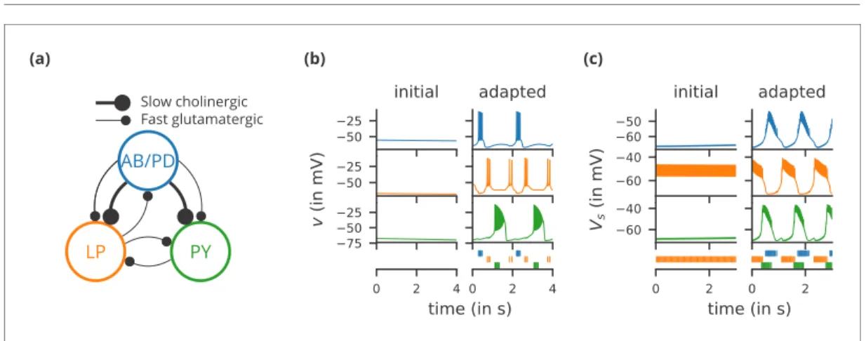
We start with a case study of a model of the pyloric network of the crustacean stomatogastric gan-glion (Figure 1a), adapted and simplified from earlier studies (Golowasch et al., 1999;Prinz et al., 2004; Prinz, 2006; O’Leary et al., 2014). This network has a small number of well-characterised neuron types – anterior burster (AB), pyloric dilator (PD), lateral pyloric (LP), and pyloric (PY) neurons – and is known to generate a stereotypical triphasic motor pattern (Figure 1b–c). Following previous studies, we lump AB and PD neurons into a single neuron type (AB/PD) and consider a circuit with one neuron of each type. The neurons in this circuit have rebound and bursting properties. We
(a) LP PY AB/PD Slow cholinergic Fast glutamatergic (b) (c)
Figure 1. Case study 1: A model of the pyloric network of the crustacean stomatogastric ganglion, inspired by several modelling papers on this subject (Golowasch et al., 1999;Prinz et al., 2004;Prinz, 2006;O’Leary et al., 2014). (a) Schematic of the modelled circuit (afterPrinz et al., 2004). The pacemaker kernel is modelled by a single neuron representing both anterior burster and pyloric dilator neurons (AB/PD, blue). There are two types of follower neurons, lateral pyloric (LP, orange), and pyloric (PY, green). Neurons are connected via slow cholinergic (thick lines) and fast glutamatergic (thin lines) synapses. (b) Activity of the simulated neurons. Membrane potential is plotted over time for the neurons in (a), using the same colour code. The bottom row shows their spiking activity in a raster plot, with spikes defined as excursions of the membrane potential over 20 mV. In the left column (‘initial’), activity is shown for 4 s after an initial settling time of 2.5 s. The right column (‘adapted’) shows the activity with fully adapted conductances (see text for details) after an additional time of 49 s. (c) Activity of the simulated neurons of a biologically detailed version of the circuit shown in (a), following (Golowasch et al., 1999). All conventions as in (b), except for showing 3 s of activity after a settling time of 0.5 s (‘initial’), and after an additional time of 24 s (‘adapted’). Also note that the biologically detailed model consists of two coupled compartments, but only the membrane potential of the somatic compartment (Vs) is shown here.
1 from brian2import *
2 defaultclock.dt = 0.01*ms;
3 Delta_T= 17.5*mV ; v_T = -40*mV ; tau = 2*ms ; tau_adapt= .02*second
4 tau_Ca = 150*ms ; tau_x = 2*second ; v_r = -68*mV ; tau_z= 5*second 5 a= 1/Delta_T**3 ; b = 3/Delta_T**2 ; c= 1.2*nA ; d= 2.5*nA/Delta_T**2
6 C= 60*pF ; S = 2*nA/Delta_T ; G = 28.5*nS
7 eqs ='''
8 dv/dt = (Delta_T*g*(-a*(v - v_T)**3 + b*(v - v_T)**2) + w - x - I_fast - I_slow)/C : volt 9 dw/dt = (c - d*(v - v_T)**2 - w)/tau : amp 10 dx/dt = (s*(v - v_r) - x)/tau_x : amp 11 s = S*(1 - tanh(z)) : siemens 12 g = G*(1 + tanh(z)) : siemens 13 dCa/dt = -Ca/tau_Ca : 1 14 dz/dt = tanh(Ca - Ca_target)/tau_z : 1 15 I_fast : amp 16 I_slow : amp 17 Ca_target : 1 (constant) 18 label : integer (constant) 19 '''
20 ABPD, LP, PY = 0,1,2
21 circuit= NeuronGroup(3, eqs, threshold='v>-20*mV', refractory='v>-20*mV', reset='Ca += 0.1',
22 method='rk2')
23 circuit.label = [ABPD, LP, PY] 24 circuit.v =v_r
25 circuit.w ='-5*nA*rand()' 26 circuit.z ='rand()*0.2 - 0.1'
27 circuit.Ca_target = [0.048,0.0384, 0.06] 28
29 s_fast = 0.2/mV; V_fast= -50*mV; E_syn = -75*mV 30 eqs_fast ='''
31 g_fast : siemens (constant)
32 I_fast_post = g_fast*(v_post - E_syn)/(1+exp(s_fast*(V_fast-v_pre))) : amp (summed) 33 '''
34 fast_synapses= Synapses(circuit, circuit, model=eqs_fast)
35 fast_synapses.connect('label_pre != label_post and not (label_pre == PY and label_post == ABPD)') 36 fast_synapses.g_fast['label_pre == ABPD and label_post == LP']= 0.015*uS
37 fast_synapses.g_fast['label_pre == ABPD and label_post == PY']= 0.005*uS 38 fast_synapses.g_fast['label_pre == LP and label_post == ABPD']= 0.01*uS 39 fast_synapses.g_fast['label_pre == LP and label_post == PY'] = 0.02*uS 40 fast_synapses.g_fast['label_pre == PY and label_post == LP'] = 0.005*uS 41
42 s_slow = 1/mV; V_slow = -55*mV; k_1 = 1/ms 43 eqs_slow ='''
44 k_2 : 1/second (constant) 45 g_slow : siemens (constant)
46 I_slow_post = g_slow*m_slow*(v_post-E_syn) : amp (summed)
47 dm_slow/dt = k_1*(1-m_slow)/(1+exp(s_slow*(V_slow-v_pre))) - k_2*m_slow : 1 (clock-driven) 48 '''
49 slow_synapses= Synapses(circuit, circuit, model=eqs_slow, method='exact') 50 slow_synapses.connect('label_pre == ABPD and label_post != ABPD')
51 slow_synapses.g_slow['label_post == LP']= 0.025*uS 52 slow_synapses.k_2['label_post == LP'] = 0.03/ms 53 slow_synapses.g_slow['label_post == PY']= 0.015*uS 54 slow_synapses.k_2['label_post == PY'] = 0.008/ms 55
56 run(59.5*second)
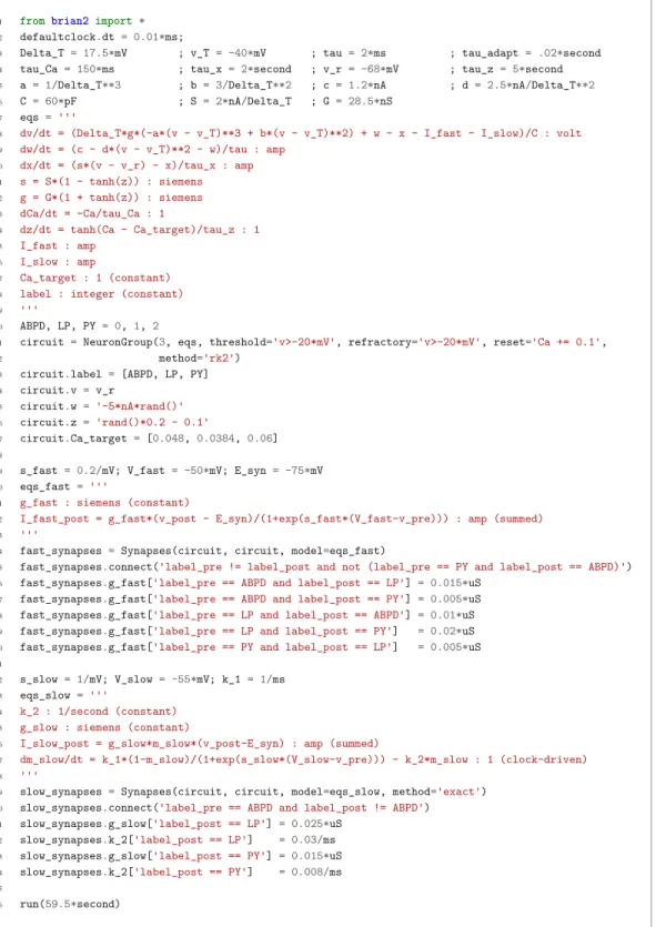
Figure 2. Case study 1: A model of the pyloric network of the crustacean stomatogastric ganglion. Simulation code for the model shown inFigure 1a, producing the circuit activity shown inFigure 1b.
DOI: https://doi.org/10.7554/eLife.47314.004
The following figure supplement is available for figure 2:
Figure supplement 1. Simulation code for the more biologically detailed model of the circuit shown inFigure 1a, producing the circuit activity shown inFigure 1c.
model this using a variant of the model proposed byHindmarsh and Rose (1984), a three-variable model exhibiting such properties. We make this choice only for simplicity: the biophysical equations originally used inGolowasch et al. (1999) can be used instead (seeFigure 2—figure supplement 1).
Although this model is based on widely used neuron models, it has the unusual feature that some of the conductances are regulated by activity as monitored by a calcium trace. One of the first design requirements of Brian, then, is that non-standard aspects of models such as this should be as easy to implement in code as they are to describe in terms of their mathematical equations. We briefly summarise how it applies to this model (see Appendix 1 andStimberg et al., 2014for more detail). The three-variable underlying neuron model is implemented by writing its differential equa-tions directly in standard mathematical form (Figure 2, l. 8–10). The calcium trace increases at each spike (l. 21; defined by a discrete event triggered after a spike, reset=’Ca + = 0.1’) and then decays (l. 13; again defined by a differential equation). A slow variable z tracks the difference of this calcium trace to a neuron-type-specific target value (l. 14) which then regulates the conductances s and g (l. 11–12).
Not only the neuron model but also their connections are non-standard. Neurons are connected together by nonlinear graded synapses of two different types, slow and fast (l. 29–54). These are unconventional synapses in that the synaptic current has a graded dependence on the pre-synaptic action potential and a continuous effect rather than only being triggered by pre-synaptic action potentials (Abbott and Marder, 1998). A key design requirement of Brian was to allow for the same expressivity for synaptic models as for neuron models, which led us to a number of features that allow for a particularly flexible specification of synapses in Brian. Firstly, we allow synapses to have dynamics defined by differential equations in precisely the same way as neurons. In addition to the usual role of triggering instantaneous changes in response to discrete neuronal events such as spikes, synapses can directly and continuously modify neuronal variables allowing for a very wide range of synapse types. To illustrate this, for the slow synapse, we have a synaptic variable (m_slow) that evolves according to a differential equation (l. 47) that depends on the pre-synaptic membrane potential (v_pre). The effect of this synapse is defined by setting the value of a post-synaptic neuron current (I_slow) in the definition of the synapse model (l. 46; referred to there as I_slow_post). The keyword (summed) in the equation specifies that the post-synaptic neuron variable is set using the summed value of the expression across all the synapses connected to it. Note that this mecha-nism also allows Brian to be used to specify abstract rate-based neuron models in addition to bio-physical graded synapse models.
The model is defined not only by its dynamics, but also the values of parameters and the connec-tivity pattern of synapses. The next design requirement of Brian was that these essential elements of specifying a model should be equally flexible and readable as the dynamics. In this case, we have added a label variable to the model that can take values ABPD, LP or PY (l. 18, 20, 23) and used this label to set up the initial values (l. 36–40, 51–54) and connectivity patterns (l. 35, 50). Human read-ability of scripts is a key aspect of Brian code, and important for reproducibility (which we will come back to in the Discussion). We highlight line 35 to illustrate this. We wish to have synapses between all neurons of different types but not of the same type, except that we do not wish to have synapses from PY neurons to AB/PD neurons. Having set up the labels, we can now express this connectivity pattern with the expression ’label_pre!=label_post and not (label_pre == PY and label_post == ABPD)’. This example illustrates one of the many possibilities offered by the equa-tion-oriented approach to concisely express connectivity patterns (for more details see Appendix 1 andStimberg et al., 2014).
Comparison to other approaches
In this case study, we have shown how a non-standard neural network, with graded synapses and adapting conductances, can be described in the Brian simulator. How could such a model be imple-mented with one of the other approaches described previously? We will briefly discuss this by focus-sing on implementations of the graded synapse model. One approach is to directly write an implementation of the model in a programming language like C++, without the use of any simula-tion software. While this requires significant technical skill, it allows for complete freedom in the defi-nition of the model itself. This was the approach taken for a study that ran 20 million parametrised
instances of the same pyloric network model (Gu¨nay and Prinz, 2010). The increased effort of writ-ing the simulation was offset by reuswrit-ing the same model an extremely large number of times. An excerpt of this code is shown inAppendix 3—figure 1c. Note that unless great care is taken, this approach may lead to a very specific implementation of the model that is not straightforward to adapt for other purposes. With such long source code (3510 lines in this case) it is also difficult to check that there are no errors in the code, or implicit assumptions that deviate from the description (as in, for exampleHathway and Goodman, 2018;Pauli et al., 2018).
Another approach for describing model components such as graded synapses is to use a descrip-tion language such as LEMS/NeuroML2. If the specific model has already been added as a ‘core type’, then it can be readily referenced in the description of the model (Appendix 3—figure 2a). If not, then the LEMS description can be used to describe it (Appendix 3—figure 2a). Such a descrip-tion is on a similar level of abstracdescrip-tion as the Brian descripdescrip-tion, but somewhat more verbose (although this may be reduced by using a library such as PyLEMS to create the description; Vella et al., 2014).
If the user chooses to use the NEURON simulator to simulate the model, then a new synaptic mechanism can be added using the NMODL language (Appendix 3—figure 2b). However, for the user this requires learning a new, idiosyncratic language, and detailed knowledge about simulator internals, for example the numerical solution of equations. Other simulators, such as NEST, are focussed on discrete spike-based interactions and currently do not come with models of graded syn-apses, and such models are not yet supported by its description language NESTML. Leveraging the infrastructure added for gap-junctions (Hahne et al., 2015) and rate models (Hahne et al., 2017), the NEST simulator could certainly integrate such models in principle but in practice this may not be feasible without direct support from the NEST team.
Case study 2: Ocular model
The second example is a closed-loop sensorimotor model of ocular movements (used for illustration and not intended to be a realistic description of the system), where the eye tracks an object (Figure 3a,b). Thus, in addition to neurons, the model also describes the activity of ocular muscles and the dynamics of the stimulus. Each of the two antagonistic muscles is modelled mechanically as an elastic spring with some friction, which moves the eye laterally.
The next design requirement of Brian was that it should be both possible and straightforward to define non-neuronal elements of a model, as these are just as essential to the model as a whole, and the importance of connecting with these elements is often neglected in neural simulators. We will come back to this requirement in various forms over the next few case studies, but here we empha-sise how the mechanisms for specifying arbitrary differential equations can be re-used for non-neuro-nal elements of a simulation.
The position of the eye follows a second-order differential equation, with resting position x0, the difference in resting positions of the two muscles (Figure 3c, l. 4–5). The stimulus is an object that moves in front of the eye according to a stochastic process (l. 7–8). Muscles are controlled by two motoneurons (l. 11–13), for which each spike triggers a muscular ‘twitch’. This corresponds to a tran-sient change in the resting position x0of the eye in either direction, which then decays back to zero (l. 6, 15).
Retinal neurons receive a visual input, modelled as a Gaussian function of the difference between the neuron’s preferred position and the actual position of the object, measured in retinal coordinates (l. 21). Thus, the input to the neurons depends on dynamical variables external to the neuron model. This is a further illustration of the design requirement above that we need to include non-neuronal elements in our model specifications. In this case, to achieve this we link the variables in the eye model with the variables in the retina model using the linked_var function (l. 4, 7, 23–24, 28–29).
Finally, we implement a simple feedback mechanism by having retinal neurons project onto the motoneuron controlling the contralateral muscle (l. 33), with a strength proportional to their eccen-tricity (l. 36): thus, if the object appears on the edge of the retina, the eye is strongly pulled towards the object; if the object appears in the centre, muscles are not activated. This simple mechanism allows the eye to follow the object (Figure 3b), and the code illustrates the previous design require-ment that the code should reflect the mathematical description of the model.
(a) xeye xobject retina motor neurons ocular muscles eye space (b) (c)
1 from brian2 import * 2
3 alpha = (1/(50*ms))**2; beta = 1/(50*ms); tau_muscle = 20*ms; tau_object = 500*ms 4 eqs_eye = '''dx/dt = velocity : 1
5 dvelocity/dt = alpha*(x0-x)-beta*velocity : 1/second 6 dx0/dt = -x0/tau_muscle : 1
7 dx_object/dt = (noise - x_object)/tau_object: 1
8 dnoise/dt = -noise/tau_object + tau_object**-0.5*xi : 1''' 9 eye = NeuronGroup(1, model=eqs_eye, method='euler')
10
11 taum = 20*ms
12 motoneurons= NeuronGroup(2, model='dv/dt = -v/taum : 1', threshold='v>1', reset='v=0', 13 refractory=5*ms, method='exact')
14
15 motosynapses = Synapses(motoneurons, eye, model='w : 1', on_pre='x0_post += w') 16 motosynapses.connect()# connects all motoneurons to the eye
17 motosynapses.w = [-0.5, 0.5] 18 19 N = 20; width = 2./N; gain = 4. 20 eqs_retina= '''dv/dt = (I-(1+gs)*v)/taum : 1 21 I = gain*exp(-((x_object-x_eye-x_neuron)/width)**2) : 1 22 x_neuron : 1 (constant)
23 x_object : 1 (linked) # position of the object 24 x_eye : 1 (linked) # position of the eye 25 gs : 1 # total synaptic conductance'''
26 retina = NeuronGroup(N, model=eqs_retina, threshold='v>1', reset='v=0', method='exact') 27 retina.v = 'rand()'
28 retina.x_eye = linked_var(eye, 'x')
29 retina.x_object = linked_var(eye, 'x_object') 30 retina.x_neuron = '-1.0 + 2.0*i/(N-1)' 31
32 sensorimotor_synapses = Synapses(retina, motoneurons, model='w : 1 (constant)',
33 on_pre='v_post += w')
34 sensorimotor_synapses.connect(j='int(x_neuron_pre > 0)') 35 # Strength scales with eccentricity:
36 sensorimotor_synapses.w = '20*abs(x_neuron_pre)/N_pre' 37
38 run(10*second)
Figure 3. Case study 2: Smooth pursuit eye movements. (a) Schematics of the model. An object (green) moves along a line and activates retinal neurons (bottom row; black) that are sensitive to the relative position of the object to the eye. Retinal neurons activate two motor neurons with weights depending on the eccentricity of their preferred position in space. Motor neurons activate the ocular muscles responsible for turning the eye. (b) Top: Simulated activity of the sensory neurons (black), and the left (blue) and right (orange) motor neurons. Bottom: Position of the eye (black) and the stimulus (green). (c) Simulation code.
Comparison to other approaches
The remarks we made earlier regarding the graded synapse in case study one mostly apply here as well. For LEMS/NeuroML2, both motor neurons and the environment could be modelled with a LEMS description. Similarly, a simulation with NEURON would require NMODL specifications of both models, using its POINTER mechanism (seeAppendix 3—figure 2) to link them together. Since NEST’s modelling language NESTML does not allow for the necessary continuous interaction between a single environment and multiple neurons, implementing this model would be a major effort and require writing code in C++ and detailed knowledge of NEST’s internal architecture.
Computational experiment level
The mathematical model descriptions discussed in the previous section provide only a partial description of what we might call a ‘computational experiment’. Let us consider the analogy to an electrophysiological experiment: for a full description, we would not only state the model animal, the cell type and the preparation that was investigated, but also the stimulation and analysis proto-col. In the same way, a full description of a computational experiment requires not only a description of the neuron and synapse models, but also information such as how input stimuli are generated, or what sequence of simulations is run. Some examples of computational experimental protocols would include: threshold finding (discussed in detail below) where the stimulus on the next trial depends on the outcome of the current trial; generalisations of this to potentially very complex closed-loop experiments designed to determine the optimal stimuli for a neuron (e.g.Edin et al., 2004); models including a complex simulated environment defined in an external package (e.g.Voegtlin, 2011); or models with plasticity based on an error signal that depends on the global behaviour of the network (e.g.Stroud et al., 2018;Zenke and Ganguli, 2018). Capturing all these potential protocols in a purely descriptive format (one that is not Turing complete) is impossible by definition, but it can be easily expressed in a programming language with control structures such as loops and conditionals. The Brian simulator allows the user to write complete computational experimental protocols that include both the model description and the simulation protocol in a single, readable Python script.
(a) step = 𝟤𝟧 𝗆𝖵 𝑣0= 𝟤𝟧 𝗆𝖵 run with 𝑣= 𝑣0 neuron spiked? decrease 𝑣0by step increase 𝑣0by step Replace step by step/2 10 iterations performed? stop yes no yes no (b)
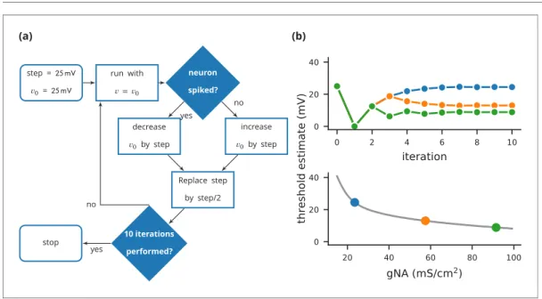
Figure 4. Case study 3: Using bisection to find a neuron’s voltage threshold. (a) Schematic of the bisection algorithm for finding a neuron’s voltage threshold. The algorithm is applied in parallel for different values of sodium density. (b) Top: Refinement of the voltage threshold estimate over iterations for three sodium densities (blue: 23.5 mS cm 2, orange: 57.5 mS cm 2, green: 91.5 mS cm 2); Bottom: Voltage threshold estimation as a function of sodium density.
Case study 3: Threshold finding
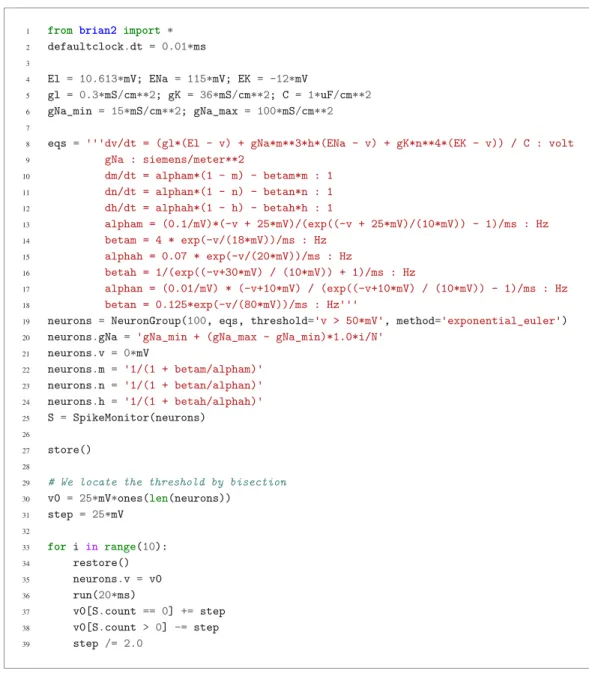
In this case study, we want to determine the voltage firing threshold of a neuron (Figure 4), mod-elled with three conductances, a passive leak conductance and voltage-dependent sodium and potassium conductances (Figure 5, l. 4–24).
To get an accurate estimate of the threshold, we use a bisection algorithm (Figure 4a): starting from an initial estimate and with an initial step width (Figure 5, l. 30–31), we set the neuron’s mem-brane potential to the estimate (l. 35) and simulate its dynamics for 20 ms (l. 36). If the neuron spikes, that is if the estimate was above the neuron’s threshold, we decrease our estimate (l. 38); if the neuron does not spike, we increase it (l. 37). We then halve the step width (l. 39) and perform the same process again until we have performed a certain number of iterations (l. 33) and converged to a precise estimate (Figure 4btop). Note that the order of operations is important here. When we
1 from brian2 import * 2 defaultclock.dt = 0.01*ms 3 4 El = 10.613*mV; ENa = 115*mV; EK = -12*mV 5 gl = 0.3*mS/cm**2; gK = 36*mS/cm**2; C = 1*uF/cm**2 6 gNa_min = 15*mS/cm**2; gNa_max = 100*mS/cm**2 7
8 eqs = '''dv/dt = (gl*(El - v) + gNa*m**3*h*(ENa - v) + gK*n**4*(EK - v)) / C : volt 9 gNa : siemens/meter**2 10 dm/dt = alpham*(1 - m) - betam*m : 1 11 dn/dt = alphan*(1 - n) - betan*n : 1 12 dh/dt = alphah*(1 - h) - betah*h : 1 13 alpham = (0.1/mV)*(-v + 25*mV)/(exp((-v + 25*mV)/(10*mV)) - 1)/ms : Hz 14 betam = 4 * exp(-v/(18*mV))/ms : Hz 15 alphah = 0.07 * exp(-v/(20*mV))/ms : Hz 16 betah = 1/(exp((-v+30*mV) / (10*mV)) + 1)/ms : Hz 17 alphan = (0.01/mV) * (-v+10*mV) / (exp((-v+10*mV) / (10*mV)) - 1)/ms : Hz 18 betan = 0.125*exp(-v/(80*mV))/ms : Hz'''
19 neurons = NeuronGroup(100, eqs, threshold='v > 50*mV', method='exponential_euler') 20 neurons.gNa = 'gNa_min + (gNa_max - gNa_min)*1.0*i/N'
21 neurons.v = 0*mV 22 neurons.m = '1/(1 + betam/alpham)' 23 neurons.n = '1/(1 + betan/alphan)' 24 neurons.h = '1/(1 + betah/alphah)' 25 S = SpikeMonitor(neurons) 26 27 store() 28
29 # We locate the threshold by bisection 30 v0 = 25*mV*ones(len(neurons))
31 step = 25*mV 32 33 for i in range(10): 34 restore() 35 neurons.v = v0 36 run(20*ms) 37 v0[S.count == 0] += step 38 v0[S.count > 0] -= step 39 step /= 2.0
Figure 5. Case study 3: Simulation code to find a neuron’s voltage threshold, implementing the bisection algorithm detailed inFigure 4a. The code simulates 100 unconnected neurons with sodium densities between 15 mS cm 2and 100 mS cm 2, following the model ofHodgkin and Huxley (1952). Results from these simulations are shown inFigure 4b.
modify the variable v in lines 37–38, we use the output of the simulation run on line 36, and this determines the parameters for the next iteration. A purely declarative definition could not represent this essential feature of the computational experiment.
For each iteration of this loop, we restore the network state (restore(); l. 34) to what it was at the beginning of the simulation (store(); l. 27). This store()/restore() mechanism is a key part of Brian’s design for allowing computational experiments to be easily and flexibly expressed in Python, as it gives a very effective way of representing common computational experimental proto-cols. Examples that can easily be implemented with this mechanism include a training/testing/valida-tion cycle in a synaptic plasticity setting; repeating simulatraining/testing/valida-tions with some aspect of the model changed but the rest held constant (e.g. parameter sweeps, responses to different stimuli); or simply repeatedly running an identical stochastic simulation to evaluate its statistical properties.
At the end of the script, by performing this estimation loop in parallel for many neurons, each having a different maximal sodium conductance, we arrive at an estimate of the dependence of the voltage threshold on the sodium conductance (Figure 4bbottom).
Comparison to other approaches
Such a simulation protocol could be implemented in other simulators as well, since they use a gen-eral programming language to control the simulation flow (e.g. SLI or Python for NEST; HOC or Python for NEURON) in similar ways to Brian. However, general simulation workflows are not part of description languages like NeuroML2/LEMS. While a LEMS model description can include a <Simu-lation> element, this is only meant to specify the duration and step size of one or several simula-tion runs, together with informasimula-tion about what variables should be recorded and/or displayed. General workflows, for example deciding whether to run another simulation based on the results of a previous simulation, are beyond its scope. These could be implemented in a separate script in a different programming language.
Implementation level
Case study 4: Real-time audio
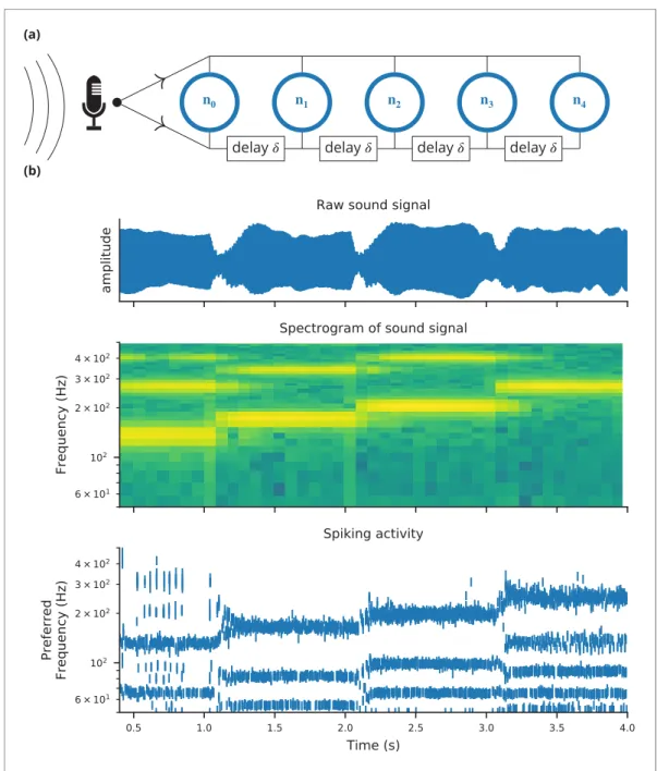
The case studies so far were described by equations and algorithms on a level that is independent of the programming language and hardware that will eventually perform the computation. However, in some cases this lower level cannot be ignored. To demonstrate this, we will consider the example presented inFigure 6. We want to record an audio signal with a microphone and feed this signal— in real-time—into a neural network performing a crude ‘pitch detection’ based on the autocorrela-tion of the signal (Licklider, 1962). This model first transforms the continuous stimulus into a sequence of spikes by feeding the stimulus into an integrate-and-fire model with an adaptive thresh-old (Figure 7, l. 36–41). It then detects periodicity in this spike train by feeding it into an array of coincidence detector neurons (Figure 6a; Figure 7, l. 44–47). Each of these neurons receives the input spike train via two pathways with different delays (l. 49–51). This arrangement allows the net-work to detect periodicity in the input stimulus; a periodic stimulus will most strongly excite the neu-ron where the difference in delays matches the stimulus’ period. Depending on the periodicity present in the stimulus, for example for tones of different pitch (Figure 6b middle), different sub-populations of neurons respond (Figure 6bbottom).
To perform such a study, our simulator has to meet two new requirements: firstly, the simulation has to run fast enough to be able to process the audio input in real-time. Secondly, we need a way to connect the running simulation to an audio signal via low-level code.
The challenge is to make the computational efficiency requirement compatible with the require-ment of flexibility. With version 1 of Brian, we made the choice to sacrifice computational efficiency, because we reasoned that frequently in computational modelling, considerably more time was spent developing the model and writing the code than was spent on running it (often weeks versus minutes or hours; cf.De Schutter, 1992). However, there are obviously cases where simulation time is a bottleneck. To increase computational efficiency without sacrificing flexibility, We decided to make code generation the fundamental mode of operation for Brian 2 (Stimberg et al., 2014). Code generation was used previously in Brian 1 (Goodman, 2010), but only in parts of the simula-tion. This technique is now being increasingly widely used in other simulators, see Blundell et al. (2018)for a review.
In brief, from the high level abstract description of the model, we generate independent blocks of code (in C++ or other languages). We run these blocks in sequence to carry out the simulation. Typically, we first carry out numerical integration in one code block, check for threshold crossings in a second block, propagate synaptic activity in a third block, and finally run post-spike reset code in a fourth block. To generate this code, we make use of a combination of various techniques from
(a)
𝐧
𝟎 𝐧𝟏 𝐧𝟐 𝐧𝟑 𝐧𝟒
delay 𝛿 delay 𝛿 delay 𝛿 delay 𝛿
(b)
Figure 6. Case study 4: Neural pitch processing with real-time input. (a) Model schematic: Audio input is converted into spikes and fed into a population of coincidence-detection neurons via two pathways, one instantaneous, that is without any delay (top), and one with incremental delays (bottom). Each neuron therefore receives the spikes resulting from the audio signal twice, with different temporal shifts between the two. The inverse of this shift determines the preferred frequency of the neuron. (b) Simulation results for a sample run of the simulation code inFigure 7. Top: Raw sound input (a rising sequence of tones – C, E, G, C – played on a synthesised flute). Middle: Spectrogram of the sound input. Bottom: Raster plot of the spiking response of receiving neurons (group neurons in the code), ordered by their preferred frequency.
symbolic mathematics and compilers that are available in third party Python libraries, as well as some domain-specific optimisations to further improve performance (see Appendix 1 for more details, orStimberg et al., 2014;Blundell et al., 2018). We can then run the complete simulation in one of two modes, as follows.
1 from brian2 import * 2 import os
3 set_device('cpp_standalone') 4
5 sample_rate = 48*kHz; buffer_size = 128; defaultclock.dt = 1/sample_rate 6 max_delay = 20*ms; tau_ear = 1*ms; tau_th = 5*ms
7 min_freq = 50*Hz; max_freq = 1000*Hz; num_neurons = 300; tau= 1*ms; sigma = .1 8
9 @implementation('cpp',''' 10 PaStream *_init_stream() { 11 PaStream* stream; 12 Pa_Initialize();
13 Pa_OpenDefaultStream(&stream, 1, 0, paFloat32, SAMPLE_RATE, BUFFER_SIZE, NULL, NULL); 14 Pa_StartStream(stream);
15 return stream; 16 }
17
18 float get_sample(const double t) {
19 static PaStream* stream = _init_stream(); 20 static float buffer[BUFFER_SIZE]; 21 static int next_sample = BUFFER_SIZE; 22
23 if (next_sample >= BUFFER_SIZE) 24 {
25 Pa_ReadStream(stream, buffer, BUFFER_SIZE); 26 next_sample = 0;
27 }
28 return buffer[next_sample++];
29 }''', libraries=['portaudio'], headers=['<portaudio.h>'], 30 define_macros=[('BUFFER_SIZE', buffer_size), 31 ('SAMPLE_RATE', sample_rate)]) 32 @check_units(t=second, result=1)
33 defget_sample(t):
34 raise NotImplementedError('Use a C++-based code generation target.')
35
36 eqs_ear = '''dx/dt = (sound - x)/tau_ear: 1 (unless refractory) 37 dth/dt = (0.1*x - th)/tau_th : 1
38 sound = clip(get_sample(t), 0, inf) : 1 (constant over dt)''' 39 receptors = NeuronGroup(1, eqs_ear, threshold='x>th',
40 reset='x=0; th = th*2.5 + 0.01', 41 refractory=2*ms, method='exact') 42 receptors.th = 1
43
44 eqs_neurons = '''dv/dt = -v/tau+sigma*(2./tau)**.5*xi : 1 45 freq : Hz (constant)'''
46 neurons = NeuronGroup(num_neurons, eqs_neurons, threshold='v>1', reset='v=0', method='euler') 47 neurons.freq = 'exp(log(min_freq/Hz)+(i*1.0/(num_neurons-1))*log(max_freq/min_freq))*Hz' 48
49 synapses = Synapses(receptors, neurons, on_pre='v += 0.5', multisynaptic_index='k') 50 synapses.connect(n=2) # one synapse without delay; one with delay
51 synapses.delay['k == 1'] = '1/freq_post' 52
53 run(10*second)
Figure 7. Case study 4: Simulation code for the model shown inFigure 6a. The sound input is acquired in real time from a microphone, using user-provided low-level code written in C that makes use of an Open Source library for audio input (Bencina and Burk, 1999).
In runtime mode, the overall simulation is controlled by Python code, which calls out to the com-piled code objects to do the heavy lifting. This method of running the simulation is the default, because despite some computational overhead associated with repeatedly switching from Python to another language, it allows for a great deal of flexibility in how the simulation is run: whenever Brian’s model description formalism is not expressive enough for a task at hand, the researcher can interleave the execution of generated code with a hand-written function that can potentially access and modify any aspect of the model. This facility is widely used in computational models using Brian. In standalone mode, additional low-level code is generated that controls the overall simulation, meaning that during the main run of the simulation it is not necessary to switch back to Python. This gives an improvement to performance, but at the cost of reduced flexibility since we cannot trans-late arbitrary Python code into low level code. The standalone mode can also be used to generate code to run on a platform where Python is not available or not practical (such as a GPU; Stimberg et al., 2018).
The choice of which mode to use is left to the user, and will depend on details of the simulation and how much additional flexibility is required. The performance that can be gained from using the standalone mode also depends strongly on the details of the model; we will come back to this point in the discussion.
The second issue we needed to address for this case study was how to connect the running simu-lation to an audio signal via low-level code. The general issue here is how to extend the functionality of Brian. While Brian’s syntax allows a researcher to define a wide range of models within its general framework, inevitably it will not be sufficient for all computational research projects. Taking this into account, Brian has been built with extensibility in mind. Importantly, it should be possible to extend Brian’s functionality and still include the full description of the model in the main Python script, that is without requiring the user to edit the source code of the simulator itself or to add and com-pile separate modules.
As discussed previously, the runtime mode offers researchers the possibility to combine their sim-ulation code with arbitrary Python code. However, in some cases, such as a model that requires real-time access to hardware (Figure 6), it may be necessary to add functionality at the target-language level itself. To this end, simulations can use a general extension mechanism: model code can refer not only to predefined mathematical functions, but also to functions defined in the target language by the user (Figure 7, l. 9–34). This can refer to code external to Brian, for example to third-party libraries (as is necessary in this case to get access to the microphone). In order to establish the link, Brian allows the user to specify additional libraries, header files or macro definitions (l. 29–31) that will be taken into account during the compilation of the code. With this mechanism the Brian simula-tor offers researchers the possibility to add functionality to their model at the lowest possible level, without abandoning the use of a convenient simulator and forcing them to write their model ‘from scratch’ in a low-level language. We think it is important to acknowledge that a simulator will never have every possible feature to cover all possible models, and we therefore provide researchers with the means to adapt the simulator’s behaviour to their needs at every level of the simulation.
Comparison to other approaches
The NEURON simulator can include user-written C code in VERBATIM blocks of an NMODL descrip-tion, but there is no documented mechanism to link to external libraries. Another approach to inter-face a simulation with external input or output is to do this on the script level. For example, a recent study (Dura-Bernal et al., 2017) linked a NEURON simulation of the motor cortex to a virtual muscu-loskeletal arm, by running a single simulation step at a time, and then exchanging values between the two systems. The NEST simulator provides a general mechanism to couple a simulation to another system (e.g. another simulator) via the MUSIC interface (Djurfeldt et al., 2010). This frame-work has been successfully used to connect the NEST simulators to robotic simulators (Weidel et al., 2016). The MUSIC framework does support both spike-based and continuous interactions, but NEST cannot currently apply continuous-valued inputs as used here. Finally, model description lan-guages such as NeuroML2/LEMS are not designed to capture this kind of interaction.
Discussion
Brian 2 was designed to overcome some of the major challenges we saw for neural simulators (including Brian 1). Notably: the flexibility/performance dichotomy, and the need to integrate com-plex computational experiments that go beyond their neuronal and network components. As a result of this work, Brian can address a wide range of modelling problems faced by neuroscientists, as well as giving more robust and reproducible results and therefore contributing to increasing reproducibil-ity in computational science. We now discuss these challenges in more detail.
Brian’s code generation framework allows for a solution to the dichotomy between flexibility and performance. Brian 2 improves on Brian 1 both in terms of flexibility (particularly the new, very gen-eral synapse model; for more details see Appendix 5) and performance, where it performs similarly to simulators written in low-level languages which do not have the same flexibility ( Tikidji-Hamburyan et al., 2017; also see section Performance below). Flexibility is essential to be useful for fundamental research in neuroscience, where basic concepts and models are still being actively investigated and have not settled to the point where they can be standardised. Performance is increasingly important, for example as researchers begin to model larger scale experimental data such as that provided by the Neuropixels probe (Jun et al., 2017), or when doing comprehensive parameter sweeps to establish robustness of models (O’Leary et al., 2015).
It is possible to write plugins for Brian to generate code for other platforms without modifying the core code, and there are several ongoing projects to do so. These include Brian2GeNN (Stimberg et al., 2018) which uses the GPU-enhanced Neural Network simulator (GeNN; Yavuz et al., 2016) to accelerate simulations in some cases by tens to hundreds of times, and Brian2CUDA (https://github.com/brian-team/brian2cuda). The modular structure of the code gener-ation framework was designed for this in order to be ready for future trends in both high-perfor-mance computing and computational neuroscience research. Increasingly, high-perforhigh-perfor-mance scientific computing relies on the use of heterogeneous computing architectures such as GPUs, FPGAs, and even more specialised hardware (Fidjeland et al., 2009; Richert et al., 2011; Brette and Goodman, 2012;Moore et al., 2012;Furber et al., 2014;Cheung et al., 2015), as well as techniques such as approximate computing (Mittal, 2016). In addition to basic research, spiking neural networks may increasingly be used in applications thanks to their low power consumption (Merolla et al., 2014), and the standalone mode of Brian is designed to facilitate the process of con-verting research code into production code.
A neural computational model is more than just its components (neurons, synapses, etc.) and net-work structure. In designing Brian, we put a strong emphasis on the complete computational experi-ment, including specification of the stimulus, interaction with non-neuronal components, etc. This is important both to minimise the time and expertise required to develop computational models, but also to reduce the chance of errors (see below). Part of our approach here was to ensure that fea-tures in Brian are as general and flexible as possible. For example, the equations system intended for defining neuron models can easily be repurposed for defining non-neuronal elements of a computational experiment (case study 2,Figure 3). However, ultimately we recognise that any way of specifying all elements of a computational experiment would be at least as complex as a fully fea-tured programming language. We therefore simply allow users to define these aspects in Python, the same language used for defining the neural components, as this is already highly capable and readable. We made great efforts to ensure that the detailed work in designing and implementing new features should not interfere with the goal that the user script should be a readable description of the complete computational experiment, as we consider this to be an essential element of what makes a computational model valuable.
Brian’s approach to defining models leads to particularly concise code (Tikidji-Hamburyan et al., 2017), as well as code whose syntax matches closely descriptions of models in papers. This is impor-tant not only because it saves scientists time if they have to write less code, but also because such code is easier to verify and reproduce. It is difficult for anyone, the authors of a model included, to verify that thousands of lines of model simulation code match the description they have given of it. An additional advantage of the clean syntax is that Brian is an excellent tool for teaching, for exam-ple in the computational neuroscience textbook ofGerstner et al. (2013). Expanding on this point, a major issue in computational science generally, and computational neuroscience in particular, is the reproducibility of computational models (LeVeque et al., 2012; Eglen et al., 2017;
Podlaski et al., 2017;Manninen et al., 2018). A frequent complaint of students and researchers at all levels, is that when they try to implement published models using their own code, they get differ-ent results. A fascinating and detailed description of one such attempt is given inPauli et al. (2018). These sorts of problems led to the creation of the ReScience journal, dedicated to publishing repli-cations of previous models or describing when those replication attempts failed (Rougier et al., 2017). A number of issues contribute to this problem, and we designed Brian with these in mind. So, for example, users are required to write equations that are dimensionally consistent, a common source of problems. In addition, by requiring users to write equations explicitly rather than using pre-defined neuron types such as ‘integrate-and-fire’ and ‘Hodgkin-Huxley’, as in other simulators, we reduce the chance that the implementation expected by the user is different to the one provided by the simulator. We discuss this point further below, but we should note the opposing view that standardisation and common implementation are advantages has also been put forward (Davison et al., 2008; Gleeson et al., 2010;Raikov et al., 2011). Perhaps more importantly, by making user-written code simpler and more readable, we increase the chance that the implementa-tion faithfully represents the descripimplementa-tion of a model. Allowing for more flexibility and targeting the complete computational experiment increases the chances that the entire simulation script can be compactly represented in a single file or programming language, further reducing the chances of such errors.
Comparison to other approaches
We have described some of the key design choices we made for version 2 of the Brian simulator. These represent a particular balance between the conflicting demands of flexibility, ease-of-use, fea-tures and performance, and we now compare the results of these choices to other available options for simulations.
There are two main differences of approach between Brian and other simulators. Firstly, we require model definitions to be explicit. Users are required to give the full set of equations and parameters that define the model, rather than using ‘standard’ model names and default parameters (cf.Brette, 2012). This approach requires a slightly higher initial investment of effort from the user, but ensures that users know precisely what their model is doing and reduces the risk of a difference between the implementation of the model and the description of it in a paper (see discussion above). One limitation of this approach is that it makes it more difficult to design tools to program-matically inspect a model, for example to identify and shut down all inhibitory currents (although note that this issue remains for languages such as NeuroML and NineML that are primarily based on standard models as they include the ability to define arbitrary equations).
The second main difference is that we consider the complete computational experiment to be fundamental, and so everything is tightly integrated to the extent that an entire model can be speci-fied in a single, readable file, including equations, protocols, data analysis, etc. In Neuron and NEST, model definitions are separate from the computational experiment script, and indeed written in an entirely different language (see below). This adds complexity and increases the chance of errors. In NeuroML and NineML, there is no way of specifying arbitrary computational experiments. One counter-argument to this approach is that clearly separating model definitions may reduce the effort in re-using models or programmatically comparing them (as inPodlaski et al., 2017).
A consequence of the requirement to make model definitions explicit, and an important feature for doing novel research, is that the simulator must support arbitrary user-specified equations. This is available in Neuron via the NMODL description format (Hines and Carnevale, 2000), and in a lim-ited form in NEST using NESTML (Plotnikov et al., 2016). NeuroML and NineML now both include the option for specifying arbitrary equations, although the level of simulator support for these aspects of the standards is unclear. While some level of support for arbitrary model equations is now fairly widespread in simulators, Brian was the first to make this a fundamental, core concept that is applied universally. Some simulators that have since followed this approach include DynaSim (Sherfey et al., 2018), which is based on MATLAB, and ANNarchy (Vitay et al., 2015). Other new simulators have taken an alternative approach, such as Xolotl (Gorur-Shandilya et al., 2018) which is based on building hierarchical representations of neurons from a library of basic components. One aspect of the equation-based approach that is missing from other simulators is the specification of additional defining network features, such as synaptic connectivity patterns, in an equally flexible, equation-oriented way. Neuron is focused on single neuron modelling rather than networks, and
only supports directly setting the connectivity synapse-by-synapse. NEST, PyNN (Davison et al., 2008), NeuroML, and NineML support this too, and also include some predefined general connectiv-ity patterns such as one-to-one and all-to-all. NEST further includes a system for specifying connec-tivity via a ‘connection set algebra’ (Djurfeldt, 2012) allowing for combinations of a few core types of connectivity. However, none have yet followed Brian in allowing the user to specify connectivity patterns via equations, as is commonly done in research papers.
Performance
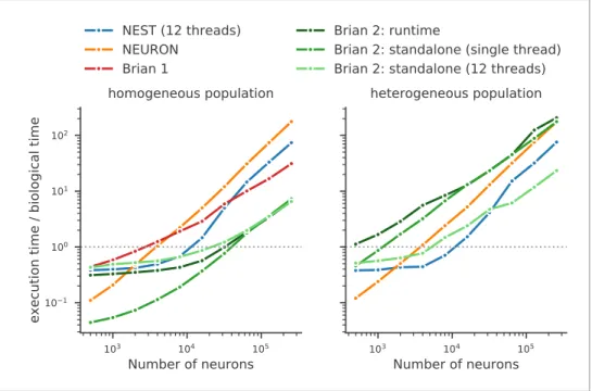
Running compiled code for arbitrary equations means that code generation must be used. This requirement leads to a problem: a simulator that makes use of a fixed set of models can provide hand-optimised implementations of them, whereas a fully flexible simulator must rely on automated techniques. By contrast, an advantage of automated techniques is that they can generate optimisa-tions for specialisaoptimisa-tions of models. For example, using the CUBA benchmark (Vogels and Abbott, 2005;Brette et al., 2007) in which all neurons have identical time constants, Brian 2 is dramatically faster than Brian 1, NEURON and NEST (Figure 8, left). This happens because Brian 2 can generate a specialised optimisation of the code since the model definition states that time constants are the same. If instead we modify the benchmark to feature heterogeneous time constants (Figure 8, right), then Brian 2 has to do much more work since it can no longer use these optimisations, while the run times for NEST and NEURON do not change.
We can make two additional observations based on this benchmark. Firstly, the benefits of paral-lelisation via multi-threading depend heavily on the model being simulated. For a large homoge-neous population, the single threaded and multi-threaded standalone runs of Brian 2 take approximately the same time, and the single threaded run is actually faster at smaller network sizes. For the heterogeneous population, the opposite result holds: multi-threaded is always faster at all network sizes.
The second observation is that the advantage of running a Brian 2 simulation in standalone mode is most significant for smaller networks, at least for the single threaded case (for the moment, multi-threaded code is only available for standalone mode).
It should be noted, however, that despite the fact that Brian 2 is the fastest simulator at large net-work sizes for this benchmark, this does not mean that Brian 2 is faster than other simulators such as NEURON or NEST in general. The NEURON simulator can be used to simulate the point neuron models used in this benchmark, but with its strong focus on the simulation of biologically detailed, multi-compartment neuron models, it is not well adapted to this task. NEST, on the other hand, has been optimised to simulate very large networks, with many synapses impinging on each neuron. Most importantly, Brian’s performance here strongly benefits from its focus on running simulations on individual machines where all simulation elements are kept in a single, shared memory space. In contrast, NEST and NEURON use more sophisticated communication between model elements which may cost performance in benchmarks like the one shown here, but can scale up to bigger ulations spread out over multiple machines. For a fairly recent and more detailed comparison of sim-ulators, seeTikidji-Hamburyan et al. (2017), although note that they did not test the standalone mode of Brian 2.
Limitations of brian
The main limitation of Brian compared to other simulators is the lack of support for running large networks over multiple machines, and scaling up to specialised, high-performance clusters as well as supercomputers. While this puts a limit on the maximum feasible size of simulations, the majority of neuroscientists do not have direct access to such equipment, and few computational neuroscience studies require such large scale simulations (tens of millions of neurons). More common is to run smaller networks but multiple times over a large range of different parameters. This ‘embarrassingly parallel’ case can be easily and straightforwardly carried out with Brian at any scale, from individual machines to cloud computing platforms or the non-specialised clusters routinely available as part of university computing services. An example for such a parameter exploration is shown in Appen-dix 4—figure 2. This simulation strongly benefits from parallelisation even on a single machine, with the simulation time reduced by about a factor of about 45 when run on a GPU.
Finally, let us note that this manuscript has focused exclusively on single-compartment point neu-ron models, where an entire neuneu-ron is represented without any spatial properties or compartmentali-sation into dendrites, soma, and axon. Such models have been extensively used for the study of network properties, but are not sufficiently detailed for studying other questions, for example den-dritic integration. For such studies, researchers typically investigate multi-compartment models, that is neurons modelled as a set of interconnected compartments. Currents across the membrane in each compartment are modelled in the same way as for point neurons, but there are additional axial currents with neighbouring compartments. Such models are the primary focus of simulators such as NEURON and GENESIS, but only have very limited support in simulators such as NEST.
Figure 8. Benchmark of the simulation time for the CUBA network (Vogels and Abbott, 2005;Brette et al., 2007), a sparsely connected network of leaky-integrate and fire network with synapses modelled as exponentially decaying currents. Synaptic connections are random, with each neuron receiving on average 80 synaptic inputs and weights set to ensure ongoing asynchronous activity in the network. The simulations use exact integration, but spike spike times are aligned to the simulation grid of 0.1 ms. Simulations are shown for a homogeneous
population (left), where the membrane time constant, as well as the excitatory and inhibitory time constant, are the same for all neurons. In the heterogeneous population (right), these constants are different for each neuron, randomly set between 90% and 110% of the constant values used in the homogeneous population. Simulations were performed with NEST 2.16 (blue,Linssen et al., 2018, RRID:SCR_002963), NEURON 7.6 (orange; RRID:SCR_ 005393), Brian 1.4.4 (red), and Brian 2.2.2.1 (shades of green,Stimberg et al., 2019b, RRID:SCR_002998). Benchmarks were run under Python 2.7.16 on an Intel Core i9-7920X machine with 12 processor cores. For NEST and one of the Brian 2 simulations (light green), simulations made use of all processor cores by using 12 threads via the OpenMP framework. Brian 2 ‘runtime’ simulations execute C++ code via the weave library, while ‘standalone’ code executes an independent binary file compiled from C++ code (see Appendix 1 for details). Simulation times do not include the one-off times to prepare the simulation and generate synaptic connections as these will become a vanishing fraction of the total time for runs with longer simulated times. Simulations were run for a biological time of 10 s for small networks (8000 neurons or fewer) and for 1 s for large networks. The times plotted here are the best out of three repetitions. Note that Brian 1.4.4 does not support exact integration for a heterogeneous population and has therefore not been included for that benchmark.
DOI: https://doi.org/10.7554/eLife.47314.011 The following source data is available for figure 8:
Source data 1. Benchmark results for the homogeneous network. DOI: https://doi.org/10.7554/eLife.47314.012
Source data 2. Benchmark results for the heterogeneous network. DOI: https://doi.org/10.7554/eLife.47314.013
While Brian is used mostly for point neurons, it does offer support for multi-compartmental models, using the same equation-based approach (see Appendix 4—figure 1). This feature is not yet as mature as those of specialised simulators such as NEURON and GENESIS, and is an important area for future development in Brian.
Development and availability
Brian is released under the free and open CeCILL 2 license. Development takes place in a public code repository athttps://github.com/brian-team/brian2(Brian contributors, 2019). All examples in this article have been simulated with Brian 2 version 2.2.2.1 (Stimberg et al., 2019b). Brian has a permanent core team of three developers (the authors of this paper), and regularly receives substan-tial contributions from a number of students, postdocs and users (see Acknowledgements). Code is continuously and automatically checked against a comprehensive test suite run on all platforms, with almost complete coverage. Extensive documentation, including installation instructions, is hosted at http://brian2.readthedocs.org. Brian is available for Python 2 and 3, and for the operating systems Windows, OS X and Linux; our download statistics show that all these versions are in active use. More information can be found athttp://briansimulator.org/.
Acknowledgements
We thank the following contributors for having made contributions, big or small, to the Brian 2 code or documentation: Moritz Augustin, Victor Benichoux, Werner Beroux, Edward Betts, Daniel Bliss, Jacopo Bono, Paul Brodersen, Romain Caze´, Meng Dong, Guillaume Dumas, Ben Evans, Charlee Fletterman, Dominik Krzemin´ski, Kapil Kumar, Thomas McColgan, Matthieu Recugnat, Dylan Richard, Cyrille Rossant, Jan-Hendrik Schleimer, Alex Seeholzer, Martino Sorbaro, Daan Sprenkels, Teo Stocco, Mihir Vaidya, Adrien F Vincent, Konrad Wartke, Pierre Yger, Friedemann Zenke. Three of these contributors (CF, DK, KK) contributed while participating in Google’s Summer of Code program.
Additional information
Funding
Funder Grant reference number Author Agence Nationale de la
Re-cherche
Axode ANR-14-CE13-0003 Romain Brette
Royal Society RG170298 Dan FM Goodman
The funders had no role in study design, data collection and interpretation, or the decision to submit the work for publication.
Author contributions
Marcel Stimberg, Conceptualization, Software, Investigation, Visualization, Methodology, Writing— original draft, Writing—review and editing; Romain Brette, Conceptualization, Software, Supervision, Funding acquisition, Investigation, Methodology, Writing—original draft, Writing—review and editing; Dan FM Goodman, Conceptualization, Software, Supervision, Investigation, Methodology, Writing—original draft, Writing—review and editing
Author ORCIDs
Marcel Stimberg https://orcid.org/0000-0002-2648-4790 Romain Brette https://orcid.org/0000-0003-0110-1623 Dan FM Goodman http://orcid.org/0000-0003-1007-6474 Decision letter and Author response
Decision letterhttps://doi.org/10.7554/eLife.47314.027 Author responsehttps://doi.org/10.7554/eLife.47314.028