electron density profiles provided by COSMIC-2
and ground-based ionosondes
G. Wautelet (1), B. Hubert (1), J.-C. Gérard (1), T. Immel (2), H. Frey (2), S. Mende (2),
F. Kamalabadi (3), U. Kamaci (3), A. Stephan (4)
(1) Laboratory for Planetary and Atmospheric Physics, University of Liège, Belgium, (2) Space Sciences
Laboratory, UC Berkeley, CA, United States, (3) University of Illinois, Urbana Champaign, IL, United
States, (4) U.S. Naval Research Laboratory, Washington D.C., United States
We compare O+ density profiles provided by ICON FUV and EUV instruments with electron density profiles measured contemporaneously by COSMIC-2 and ionosondes.
Co-located and simultaneous observations are compared on statistical grounds, and the differences between the several methods are investigated.
Particular attention is given to the most important variables, such as the altitude and the density of the F-peak, NmF2 and hmF2.
The time interval considered in this study nearly covers the whole ICON public data availability period, which started on November 16, 2019.
The total number of comparisons is nearly 60.000 cases for FUV/C2, more than 12.000 cases for EUV/C2, and more than 500 cases for FUV or EUV/ionosonde comparison.
The latter lower number of cases is due to the necessary manual screening and scaling of ionogram sequences to ensure reliable ionosonde profiles, while COSMIC-2 data are carefully selected using an automatic quality control algorithm.
ICON flies at an altitude of about 590 km on a nearly-circular 27° inclination orbit.
ICON-FUV: nighttime O density profiles
Nighttime measurement of OI-135.6 nm emission corresponding to the radiative recombination of O Six vertical profiles (stripes) every 12s
Limb scans
Data Product L2.5, file version 3
ICON-EUV: daytime O density profiles
Daytime measurement of two ionized oxygen emissions at 83.4 and 61.7 nm One vertical profile every 12s
Limb scans
Data Product L2.6, file version 2
Ionosonde: electron density profiles
Vertical incidence soundings performed in radio frequencies between 1 and 30 MHz
Direct measurement of the plasma frequency fof2. An inversion is needed to retrieve the true reflection height hmF2
14 fixed ground stations, mainly in the northern hemisphere at mid-latitudes, have been used in this study. Only one station is located in the low-latitude ionosphere. This observational bias has to be taken into account when discussing ionosonde results
Each ionogram sequence is manually scaled by the authors thanks to the SAO-X software developed by University of Massachusetts, Lowell.
COSMIC-2 (C2): electron density profiles
Radio occultation of GNSS satellites using GNSS receivers onboard Low-Earth Orbit (LEO) spacecraft The six LEO satellites are on low-inclination orbit so that C2 profiles also observe low and mid latitudes GNSS-TEC (Total Electron Content) is an integrated quantity that has to be inverted to get the electron density profile
C2 mission was launched in 2019 and provides more than 3.000 ionospheric profiles per day "IonPrf" product (provisional space-weather dataset)
+
+
Data availability
FUV: Dec. 1, 2019 (DOY 335) to Jul. 4, 2020 (DOY 186) EUV: Dec. 1, 2019 (DOY 335) to Apr. 17, 2020 (DOY 108) Ionosonde: campaign of 16 days in January and February 2020 COSMIC-2: from Sep. 30, 2019 ongoing
Finding the conjunctions
FUV location: tangent point position at the density peak EUV location: tangent point at 300 km altitude ionosonde location: station location
COSMIC-2 location: tangent point position at the density peak maximum distance between locations = 500 km
maximum time difference between measurements = 15 min
Data selection
FUV: selection of quality flag == 1
FUV: Solar Zenith Angle (SZA) > 110° (ensure nighttime conditions up to 400 km altitude)
FUV: rejection of observations affected by conjugate photo-electrons → rejection of data with SZA at magneto conjugated point < 110°
EUV: rejection of χ2 values > 0.5E+11 e/m²
ionosonde: manual scaling of ionogram sequences and rejection of unreliable ionograms
COSMIC-2: quality control based on Chapman adjustment and rejection of "bad profiles" based on "observations vs fit" differences
1. COSMIC-2 difference maps
5° x 5° binning of ΔNmF2 and ΔhmF2 and averaging within each bin for FUV-COSMIC-2 comparison.
Figure 1. 5°x5° bins of averaged ΔNmF2 (top) and ΔhmF2 (bottom) for C2-FUV comparison. Data gap over South America corresponds to the South Atlantic Anomaly (SAA). Contour lines correspond to geomagnetic inclination, in degrees.
Analysis
ΔNmF2 and ΔhmF2 ar mostly positive at all locations
ΔNmF2 are mostly homogeneously distributed on the map, despite the existence of some clusters (e.g. Carribean, Hawaii and East Pacific sectors) which should be further investigated
ΔhmF2 are larger at mid-latitudes, especially in the northern hemisphere
2. Summary statistics
Figure 2a. Histogram of ΔNmF2 for FUV-ionosonde comparison
Figure 2c. Histogram of ΔhmF2 for FUV-ionosonde comparison
Figure 2d. Histogram of ΔhmF2 for FUV-C2 comparison
Analysis
Except for Figure 2a, the quasi-Gaussian shape of the histograms validate the descriptive statistics in Table 1 (mean and std. dev.)
absolute values for ΔhmF2
FUV NmF2 is slightly larger than that of C2 and ionosonde, with a mean value of 9.6E+10 e/m³ FUV hmF2 is larger than that of C2 and ionosonde, with mean values of 15 km and 38 km respectively Relative differences for NmF2 are explained by a very low background ionosphere due to solar minimum conditions.
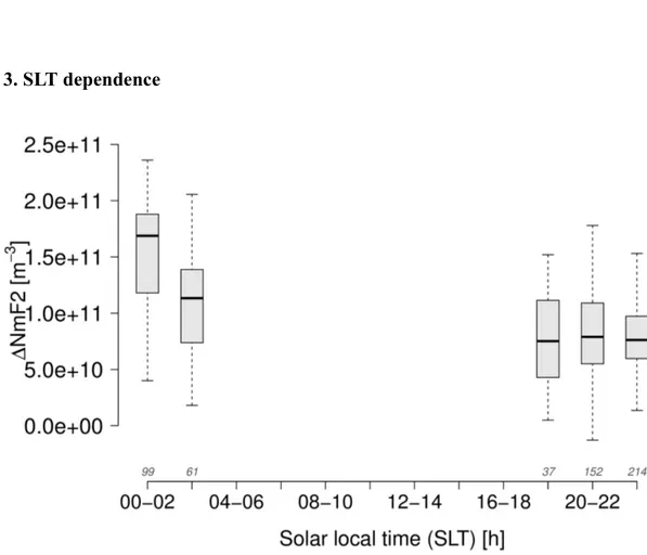
3. SLT dependence
Figure 3a. Boxplots of ΔNmF2 for FUV-ionosonde comparison for six SLT intervals. Boxes represent the quartiles, the median is the thick black line inside the box while the wiskers are located at 1.5 times the interquartile range. The small numbers in italic below the boxplots correspond to the sample size. Outliers are removed from the panel for the sake of clarity.
Figure 3b. Same as for Figure 3a but for FUV-C2 comparison.
Figure 3d. Same as for Figure 3c but for FUV-C2 comparison.
Analysis
Solar Local Time has a non negligible influence on the discrepancies between FUV and the other data sources. The smallest differences in both NmF2 and hmF2 are observed during the deep night, several hours after sunset (from 22 to 02-04 LT).
There is a disagreement in ΔNmF2 for the 00-02 LT slice between C2 and ionosonde datasets. It may be due to an isolated case in the ionogram database: ionosonde sample is < 100 while that related to the C2 dataset is 20 times larger.
The hmF2 differences with respect to C2 seem to converge to the value of about 10-15 km during the very deep night, while mean differences up to 80 km can be observed before sunrise (04-06 LT slice). This effect is not visible in the ionosonde dataset, maybe because of the small number of coincidences for some SLT slices. More generally, hmF2 comparisons with C2 are more reliable due to their very large sample size and the ubiquity of the conjunctions.
1. COSMIC-2 difference maps
5° x 5° binning of ΔNmF2 and ΔhmF2 and averaging within each bin for EUV-COSMIC-2 comparison.
Figure 4. 5°x5° bins of averaged ΔNmF2 (top) and ΔhmF2 (bottom) for C2-EUV comparison. Data gap over South America corresponds to the South Atlantic Anomaly (SAA). Contour lines correspond to geomagnetic inclination, in degrees
.
Analysis
ΔNmF2 values are generally negative (blue) at the global scale. However, values close to zero (greenish pixels) and positive values (yellow pixels) are observed above 30° dip inclination in the northern hemisphere. There is a cluster of positive ΔNmF2 values (yellow pixels) in the Pacific sector, especially around Hawaii, between 30° and 45° dip inclination
ΔhmF2 are mostly positive at all longitudes and no obvious latitude or longitude dependence can be deduced from Figure 4.
Table 2. Mean and standard deviation of ΔNmF2 and ΔhmF2 for EUV-C2 and EUV-ionosonde comparisons
Figure 5b. Histogram of ΔNmF2 for EUV-C2 comparison
Figure 5d. Histogram of ΔhmF2 for EUV-C2 comparison
Analysis
Unlike for the FUV analysis, the shape of all histograms cannot be assimilated to a Gaussian curve. We should then be careful while interpreting mean and std. dev. results for these cases, especially when considering ΔhmF2 between EUV and ionsonde (Figure 5c).
Ionosonde and COSMIC-2 results lead to similar conclusions for NmF2 in terms of relative numbers (about -50% in average), but not in absolute value which varies by a factor of 2. This is explained by the the reduced size of the ionosonde dataset, characterized by low NmF2 values in Jan - Feb. 2020. Remind that most of ionsondes are located at mid-latitudes, shifting the average NmF2 towards lower values.
HmF2 results are also very similar between C2 and ionosonde, with 5 km difference only between the two comparison datasets on average. However, as mentioned above, using a mean value for the ionosonde dataset is not statistically rigourous given the bimodal distribution of Figure 5c. More ionograms are needed to confirm this results.
Figure 6a. Boxplots of ΔNmF2 for EUV-ionosonde comparison for six SLT intervals. Boxes represent the quartiles, the median is the thick black line inside the box while the wiskers are located at 1.5 times the interquartile range. The small numbers in italic below the boxplots correspond to the sample size. Outliers are removed from the panel for the sake of clarity.
6b). These observations are not compatible with that related to the ionosonde dataset and it cannot be concluded to a relation between ΔNmF2 and SLT.
For the ionosonde dataset, the hmF2 difference is the largest around noon and tends towards zero near the terminator (Figure 6c). The C2 dataset suggests that there is a slight linear trend of ΔNmF2 with local time (Figure 6d). Like for NmF2, these two contradictory observations prevent drawing an obvious and unique relationship betweenSLT and ΔhmF2.
DISCUSSION: A GEOMETRIC APPPROACH
There is a large variability about the mean and median values as observed in histograms and boxplots.
In the case of line-of-sight integrated observations such as those from C2 and ICON, the observing geometry is of some importance. The regions crossed by both lines of sight should therefore preferably be similar, in order to produce comparable observations, i.e. both lines-of-sight should be as parallel as possible.
→ geometric filter: selection of lines of sight for which the azimut difference between ICON and C2 is < 30°
New summary statistics:
Table 3. New FUV and EUV vs COSMIC-2 summary statistics considering azimut filtering: Δazimut < 30°
Comparison of these results with that of Tables 1 and 2
FUV: ΔNmF2 sees its mean and std. dev. significantly decrease in absolute value but not in a relative way. FUV: ΔhmF2 is significantly larger when considering the azimuth filtering.
EUV: Despite a slight decrase of the mean values for ΔNmF2, the other parameters are roughly identical In conclusion: the azimut filtering does not seem to significantly decrease the differences beween ICON and C2, contrary to our expectations. More work is needed to better understand the causes of such discrepancies.
SUMMARY AND FUTURE WORK
This work is the first large-scale comparison of ICON FUV and EUV O+ density profiles with external data sources
COSMIC-2 and ionosonde provide similar trends but absolute and relative values of the differences can differ FUV provides slightly larger NmF2 values than external data, the difference being increased during the early morning hours
ABSTRACT
In October 2019, NASA-ICON was launched to observe the low-latitude ionosphere using in-situ and remote sensing instruments, from a LEO circular orbit at about 595 km altitude. The six satellites of the radio-occultation program COSMIC-2 were also successfully launched and currently provide up to 3000 electron density profiles on a daily basis since October 1, 2019. Besides, the network of ground-based ionosondes is constantly growing and allows retrieving very accurate measurements of the electron density profile up to the peak altitude. These three sources of scientific observation of the Earth ionosphere therefore provide a very complementary set of data.
We compare O density profiles provided during nighttime by the FUV instrument and during daytime by the ICON-EUV instrument against electron density profiles measured by COSMIC-2 and ionosondes. Co-located and simultaneous observations are compared on statistical grounds, and the differences between the several methods are investigated. Particular attention is given to the most important variables, such as the altitude and the density of the F-peak, hmF2 and NmF2. The time interval considered in this study covers the whole ICON data availability period, which started on November 16, 2019. Manual screening and scaling of ionograms is performed to ensure reliable ionosonde data, while COSMIC-2 data are carefully selected using an automatic quality control algorithm.
A particular attention has been brought to the geometry of the observation, because the line-of-sight integration of both airglow and radio-occultation measurements assimilates horizontal and vertical gradients. As a consequence, the local density profiles obtained by inversion of the ICON and COSMIC-2 observation cannot be exactly assimilated to vertical
measurements, such as vertical incidence soundings from ionosondes. This slightly limits the reach of the interpretation of the comparison between data of different origin. However, using similar observing geometries, the comparison of ICON and COSMIC-2 data does nevertheless provide very reliable and valuable comparisons.
Wautelet et al., First ICON O density profiles comparison to ground and space-based measurements, Journal of Geophysical Research: Space Physics, in prep