New One Shot Engine Validation Based on Aerodynamic Characterization and Preliminary Combustion Tests

HAL Id: hal-02874822

https://hal.archives-ouvertes.fr/hal-02874822

Submitted on 19 Jun 2020

HAL is a multi-disciplinary open access archive for the deposit and dissemination of sci-entific research documents, whether they are pub-lished or not. The documents may come from teaching and research institutions in France or abroad, or from public or private research centers.

L’archive ouverte pluridisciplinaire HAL, est destinée au dépôt et à la diffusion de documents scientifiques de niveau recherche, publiés ou non, émanant des établissements d’enseignement et de recherche français ou étrangers, des laboratoires publics ou privés.

New One Shot Engine Validation Based on Aerodynamic

Characterization and Preliminary Combustion Tests

M. Di Lorenzo, Pierre Brequigny, Christine Mounaïm-Rousselle, Fabrice

Foucher

To cite this version:

M. Di Lorenzo, Pierre Brequigny, Christine Mounaïm-Rousselle, Fabrice Foucher. New One Shot Engine Validation Based on Aerodynamic Characterization and Preliminary Combustion Tests. Flow, Turbulence and Combustion, Springer Verlag (Germany), In press, �10.1007/s10494-020-00185-3�. �hal-02874822�

NEW ONE SHOT ENGINE VALIDATION

BASED ON AERODYNAMIC

CHARACTERIZATION AND PRELIMINARY

COMBUSTION TESTS

M. Di Lorenzo 1, P. Brequigny 1, F. Foucher 1, C. Mounaim-Rousselle 1

1

Univ. Orléans, INSA-CVL, PRISME, EA 4229, F45072, Orléans, France

marco.di-lorenzo@etu.univ-orleans.fr

Abstract

Among the technological solutions proposed to reduce air pollutants and greenhouse gas emissions, the so-called “downsizing” operating mode for Internal Combustion Engines is considered one of the most promising. By boosting the intake air pressure, this operating mode achieves higher efficiency, thus reducing pollutant emissions. Modelling the combustion process in these drastic conditions (high pressure, high temperature and high dilution rate) remains challenging, however, as classical models of premixed turbulent combustion prove insufficiently robust The present work presents, characterizes and validates a dedicated apparatus based on the innovative NOSE (New One Shot Engine) to investigate turbulent premixed flames under these drastic conditions. The great flexibility of NOSE can generate different internal flow aerodynamic conditions as well as temperature and pressure values, up to a turbulent intensity of 3.3 m/s at 21 bar and 585 K, so at a Ka number ~10, with a characteristic integral length of 2 mm. The first milestones of the present work focus on the aerodynamic characterization of NOSE with different ad-hoc studied configurations. The validation of the setup is supported by some examples of the combustion tests performed.

Keywords: Rapid Compression Machine, Karlovitz number, High-pressure Combustion, Highly Diluted Flames, Turbulent Flames

1. Introduction

Environmental protection, energy consumption and control of pollutant emissions are important issues that urgently need to be tackled worldwide. Strong efforts are taking place in different research fields to assist in solving these global issues. As the transportation sector still largely uses fossil fuels, it contributes a significant percentage of global greenhouse gas emissions. In 2016 this percentage was 20%

for EU countries and, of this, light duty vehicles were the largest source of GHG. Despite the increasing development and implementation of alternative energy sources and systems, internal combustion engines (ICEs) still represent the

reference technological solution in the automotive sector. Faced with increasingly strict standards, the current primary target in automotive research is to increase efficiency while reducing and controlling pollutant emissions. One of the major routes towards a high efficiency Spark-Ignition (SI) engine is downsizing, which consists in increasing the engine load through displacement reduction and

turbocharging. As this leads to an increase in initial temperature and pressure, a high level of dilution has to be used to avoid abnormal combustion. As the stability of premixed turbulent combustion is strongly affected by dilution, increasing the tolerance of SI engines to high dilution remains a major technical challenge. The prediction of engine behavior in these working mode conditions remains insufficiently accurate. Most turbulent premixed combustion models are based on the flamelet regime assumption [1]. However, recent work by Mounaïm-Rousselle et al. [2] pointed out a possible breach of this regime in Spark-Ignition engines for the operating conditions of downsized engines with high rates of exhaust gas recirculation (EGR) [3], [4]. According to the flamelet regime, the flame is considered as asymptotically thin and locally laminar even if turbulence can wrinkle the flame surface [5], [6]. To provide a more accurate and reliable predictive model for future SI engine design, it is necessary to overcome the lack of experimental data that are currently gathered in conditions that are quite far from real operating conditions. Currently, it is hard to measure in actual engines because on top of the turbulent process they suffer from cycle-to-cycle variations which make the analysis even more difficult since they are linked to several interacting complex phenomenon, such as mixture preparation, heat losses (different if optical or metallic engines are used), spark-ignition, etc. Hence a lot of studies are typically carried out in spherical vessel since they offer the

following advantages:

 Accurate control of the mixture composition, including EGR.

 Minimization of temperature stratification occurrence.

 Knowledge of internal main parameters and of turbulence properties.

However, usually spherical vessels are limited in their ability to reach high initial thermodynamic conditions. Moreover, the generation of high turbulence intensity with low integral length scales remains a tough issue [8]–[10]. Even if a rapid compression set-up with optical access can overcome these limits, reproducing real engine-like conditions, it cannot offer the aforementioned diagnostic advantages and suffers from cycle to cycle variations which prevent from isolating the turbulence and the variations related to the mechanics. Hence the idea of a new experimental setup offering both high thermodynamic conditions and advantages of spherical vessel makes sense. The New One Shot Engine [7], whose features are presented in Section 2, represents an innovative solution to simulate engine-like conditions in the combustion chamber. This first study with this new experimental setup in order to validate the hypothesis of quasi-isotropic and homogeneous turbulence.

The experimental investigation of NOSE consists, first, of a repeatability

evaluation to assess the test-to-test reproducibility of the ambient conditions and the stability of the designed trajectory. Then, for each experimental condition, PIV (Particle Image Velocimetry) is used to evaluate the internal flow field and its evolution, especially during the ‘constant plateau’ where pressure and

temperature targets are reached. Twenty tests were performed for each set-up configuration. Combustion tests are useful to optimize the spark ignition phasing as it needs to burn within the ‘plateau’ but also to avoid the shift of the flame upward or downward according to the temporal evolution of the flow. In the case of highly turbulent flames, a large number of tests are usually necessary to gather enough meaningful data, to characterize the turbulent nature of the flame

propagation. Lastly, each experimental point needs to be tested in reactive conditions. This was performed using the double-view Schlieren technique to image the flames.

1.1. Fundamental Theory

The structure of premixed flames depends on the interaction between the flame front and the turbulent eddies. As a function of this interaction process, different combustion regimes were identified as in the well-known Peters-Borghi diagram [1], [11], [12], [13], where the Karlovitz number ), the Damkohler number ( and the Reynolds number ( ) are the main fundamental parameters. By

naming the turbulent intensity, corresponding to the equivalent turbulent intensity of the turbulent kinetic energy , the chemical scale, the Taylor scale and the Kolmogorov scale are defined as:

with the laminar flame thermo-diffusive thickness, the unstretched laminar burning velocity, the integral length scale, the kinematic viscosity and the dissipation rate of the turbulence kinetic energy. Then the characteristic

nondimensional numbers can be estimated:

For the sake of completeness, the expression of the rate of dissipation of the turbulence kinetic energy, , and the expression of the Kolmogorov length scale,

, are the following:

and, thus, the explicit form of the Karlovitz number is:

Eq. (3) and (4) clarify the dependence on turbulence and laminar properties of the flame. This expression of the Karlovitz number is usually solved using the thermo-diffusive flame thickness. Using other more restrictive definitions of the flame thickness (such as that of Blint [14]) yields higher Karlovitz numbers due to the increase in the flame thickness estimation. For the sake of consistency, in the following, the diffusive flame thickness will be used to plot points on a Peters-Borghi diagram. Each point on this logarithmic diagram depends on the interaction between the turbulence and the flame front. In particular, the ratios and are taken into account, and the hypothesis of Homogeneous Isotropic Turbulence (HIT) is assumed.

1.2. Characteristics of the Turbulence

Homogeneous Isotropic Turbulence (HIT) is an idealized condition of a turbulent flow. It enables the impact of turbulence on a system to be studied using a

simplified mathematical approach without neglecting any basic physical process [15]. Homogeneity is defined as the property of the statistical quantities to be invariant with respect to the translation of the reference system, while isotropy ensures independence from rotation and reflection of the coordinate axes. As it is an idealized condition, HIT does not exist in real systems. Moreover, it is

normally even difficult to reproduce similar conditions in an experimental setup. In order to obtain a real flow close to the HIT condition, with a good

approximation, several setup concepts have been proposed and used. The most common strategy is to let a steady flow pass through a grid or a mesh [16], [17]. The 2D flow fields parallel to the grid result in a good approximation of HIT conditions, but an intrinsic anisotropy exists due to the turbulence spatial decay after the grid. The strategy adopted in the present work consists in using a grid to modify the initial conditions of the normal recirculation phenomenon inside the chamber, due to the wall effects. In other words, the grid was not designed to directly generate a specific turbulence. On the contrary, the desired turbulent structures appear later, as result of the grid perturbation on the flow before the effect of wall confinement and recirculation. The aim is to obtain a 3D turbulence that is close to the HIT condition.

2. Experimental Setup

The working principle of NOSE consists in using an ideally adiabatic compression process to accurately reproduce high temperature and pressure conditions. The apparatus is fully schematized in Figure 1. As the name suggests, the machine does not operate cyclically. Starting from relatively low initial temperature and pressure, it is possible to recreate, and maintain for a sufficient interval of time, extremely high pressure and temperature at the end of the compression phase. A purposely-developed design is necessary to this end, together with a sophisticated control system, in order to mitigate the effects of the dynamicity of the apparatus. This setup was fully described in [7]. The

conditions. A dedicated chamber was designed with an internal spherical shape (40 mm radius) and four cylindrical quartz windows (18 mm radius and 25 mm thickness). The ignition is driven thanks to two tungsten electrodes and four resistive heaters can be used to warm the chamber up to 473 K. A smooth connection or a solid grid can be used to modify the internal aerodynamic of the compressed gaseous mixture. If required, the compression ratio exploitable range can be further decreased by adding a purpose-designed extension that drastically increases the initial and final volumes. Considering the ad-hoc crafted combustion chamber and a stroke of 182.15 mm, the standard setup has an initial volume Vi =

3729.72 cm3, and a final volume Vf = 381.52 cm3. We will refer to this setup as

the Small Volume (SV) configuration with a resulting CR of 9.78. With the extension, the initial volume is 6747.72 cm3, and the final volume 3399.52 cm3. We will refer to this setup as Large Volume (LV), with a CR of 1.99. Figure 2 shows a scheme of the two configurations, while Figure 3 presents the combustion chamber and details of the turbulence grid and the removable thermocouple. Further details on the grid design and impact on the flow will be given in the following Section 3.1.

Figure 2. Scheme of the two NOSE configurations: Large Volume (LV) on the left and Small Volume (SV) on the right.

The piston is driven by a brushless DC motor (PHASE Automation U31340) coupled with a high-performance electric driver motor (PHASE Automation AxM300-400), following the trajectory designed by the operator. The driven force must counteract the pressure increase and the internal friction of the oil-lubricated cylinder-piston system. For this reason a highly accurate closed-loop velocity feedback function was developed for NOSE, allowing a real-time control on piston velocity during the compression process. A trajectory example is given in Figure 4. The main target is usually to slow down the piston near the TDC in order to reach that point slowly, maintaining the obtained thermodynamic conditions for few milliseconds and reducing noise and vibrations of the system. The two velocity traces in Figure 4 correspond to the rotational speed used by the controller to shape the trajectory on one side and the measured one on the other side. These traces are directly related to the control system that includes the way in which trajectories are designed, the electric motor capability, the PID controller parameters and the response of the system (that depends on internal friction, inertia and compression ratio).

Figure 3. Details of the combustion chamber, pressure transducer and thermocouple (top); details of the grid designed for turbulence generation (bottom).

Figure 4. Example of trajectory (SV configuration with standard trajectory).

The minimum velocity is between 50 and 100 rpm, the duration of the ‘plateau’ (that is the range in which conditions inside the chamber are almost constant) strictly depends on the initial parameters and on the trajectory and can range from 5-10 to 25-30 ms. Maximum initial temperature is 473 K for the combustion chamber and 373 K for the cylinder/piston system. Before each run the piston is positioned at the BDC and a vacuum is created. The initial gas mixture

composition is obtained using four BROOKS® model 5860S gas flow meters, to supply N2, O2, CO2, CH4, etc., and two Bronkhorst mini CORI-FLOW (30 g/h)

liquid flow meters, to inject water and liquid fuels. Liquid components are carried by the gas flow inside a heated capillary tube, ensuring vaporization. A manual valve feeds a supplementary seeder line, if PIV tests need to be performed. Three other valves control purge, exhaust and vacuum pump lines. The feedback of three temperature sensors is used to monitor the temperature of the cylinder, of the chamber and of the internal gases. Maximum initial pressure is 10 bar. A high-pressure sensor is used to follow the high-pressure evolution inside the chamber during the engine shot (up to 100 bar). Gas temperature evolution inside the chamber can be tracked using a 13 µm K-type (CHROMEGA™/ALOMEGA™) thermocouple that can be displaced along the chamber. It is composed of a protective movable ceramic casing, with two ducts in which the two metal wires are accommodated. The joint is exposed to the flow. Pressure and temperature evolution, crank angle,

velocity feedback and electric motor response are recorded as a function of time through a National Instruments Compact RIO at 250 kHz. Ad-hoc configured Lab-View software is used to control the system, change the piston velocity trajectories, monitor the main parameters and phase the trigger signals. After each test, the gases are expelled and dry air at 7 bar is used to clean the residuals.

2.1. Optical setups

The PIV setup requires a High Speed Phantom v1610 camera, a high frequency and high power laser Quantronix Dual Hawk HP (9.4 mJ/pulse, 532 nm

wavelength and 120 ns pulse duration), a seeder and a set of lens. The scheme of this setup is reported in Figure 5. A cylindrical lens with a focal length of 50 mm is first used to expand the laser beam in the vertical direction. The subsequent spherical lens, with a focal length of 500 mm, changes the beam divergence slightly in the vertical direction, causing the convergence to the focal point (at the combustion chamber center) in the horizontal direction. The result is a 1 mm thick laser sheet across the combustion chamber cross-section. The high-speed camera is positioned perpendicularly to this laser plane in order to record the light scattered by the seeding particles.

Figure 5. Scheme of the PIV set-up.

The double-frame high-speed PIV analysis is performed with a short dt of , a resolution of 768x768 px2 and a mm/pixel ratio of 18.6 µm/px. The camera and

the laser are controlled by the dedicated software DAVIS (LaVision). Post-processing is first performed on DAVIS, computing the vector fields. Then the statistical analysis is performed in MATLAB.

Double-View Schlieren (DVS) imaging is used to simultaneously obtain two different views of the flame propagation recorded in just one High Speed Phantom v1610 camera; details are reported in [18] and a scheme of the setup is given in Figure 6. Two LED lamps, with a pinhole of 1 mm, are used as light sources and a set of mirrors, both planar and convex, ensures that the light beam is, respectively, well-oriented and parallel. The light is first directed to a parabolic mirror, with a focal length of 500 mm, that is the same distance from the light source, obtaining a parallel beam. After the combustion chamber, another parabolic mirror, equal to the first, is used to converge the light to the cutoff point. Through two other plano-convex lenses the light beam path is optimized to correctly impact the camera objective with the optimal size. For the preliminary tests the resolution was 1200x800 px2, the magnification ratio was 91.03 µm/px, and the frame rate was 5000 fps.

3. Results

During the development and optimization phase of NOSE, three main

configurations were identified: one low temperature and low pressure (LTLP) condition (using the LV configuration), and two high temperature and high pressure (HTHP) conditions (using the SV configuration). The two HTHP differ in the resulting turbulence intensity. In one case the piston starts at the BDC (180° CAD) and normally performs one revolution before returning to the initial

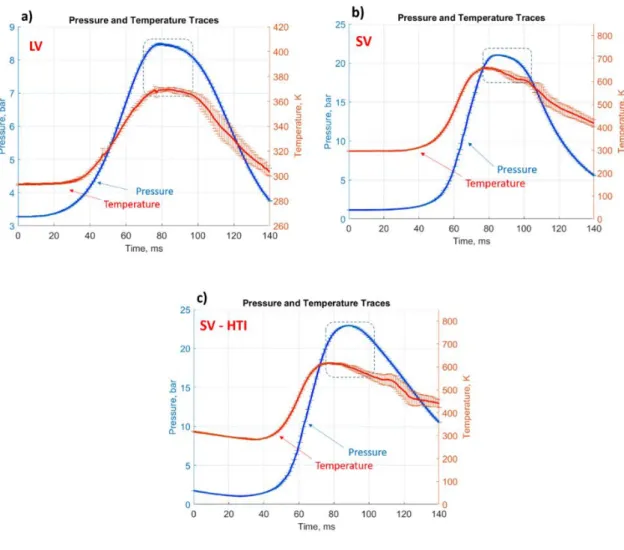
position. In the other case, a new trajectory was designed to increase the turbulent kinetic energy (TKE) without changing CR (and thus the plateau thermodynamic parameters). Before starting, the piston is slowly backward to 80° CAD so that it is possible to take advantage of the initial non-zero velocity of the piston. In this manner it is possible to better counteract the system internal resistance by accelerating more before sharply slowing down at TDC. This high turbulent intensity configuration will be called SV-HTI hereafter. Figure 7 shows the repeatability tests performed for these three configurations. The error bars are generally quite small except for the temperature curve starting from the beginning of the expansion phase. This is assumed to be the effect of the thermocouple design. The pressure increase during the compression phase compresses the gas inside the ceramic tube. Then, air is blown out by the pressure decrease at the beginning of the expansion phase, directly impacting the thermocouple. This partial lack of accuracy can be considered unimportant, however, since it always occurs after the plateau.

Figure 7. Operating conditions and repeatability tests.

3.1. Aerodynamic Characterization

The grid used for the turbulence generation presents 5 holes, one of which is centered and without inclination. The axes of the other 4 holes are inclined by 27° externally directed with respect to the central axis. Figure 8 evidences the effect of the grid on the flow. Two extreme cases are reported: the first one, on the left, is the LV configuration without the grid. The flow field displays the aerodynamics near the end of the compression phase: the velocity field is almost uniform along the x direction. Velocity vectors are well-oriented in the same direction and only a difference in magnitude is observed along the y direction. Moreover, the average absolute velocity in the center of the chamber is relatively low. This result is due to the additional inertial effect caused by the additional volume of the LV setup. In fact, without the grid, the very low compression rate and large inertial volume are not sufficient to self-generate turbulence other than at the very end of the

plateau. The second case, on the right, is a SV configuration with the grid. At the

is clearly visible. The other jets are outside the laser sheet and it is therefore possible to detect only their indirect effects on the flow field. These include the recirculation of the side jets impacting the upper part of the chamber (with a certain inclination) and coming back to the center with lower velocities in the opposite direction with respect to the central jet.

Figure 8. Effect of the grid on the flow: a) velocity flow field without the grid; b) jets formation due to the grid effect on the flow.

PIV analysis and subsequent turbulence statistical post-processing required high spatial resolution to increase the precision of the evaluation of the integral lengths. The window used for turbulence statistical analysis is 14.29x14.29 mm2 centered with respect to the center of the chamber. Figure 8 shows this reduced window as a red square. The recording frequency is 10 kHz so, assuming a plateau of 20 ms, 201 velocity fields per test are available. For each configuration 20 tests were performed. The turbulence is not continuously forced and it cannot be considered globally stationary. In order to have an idea of the turbulence evolution during the

plateau, an ensemble average approach is used. One can define the generic

velocity component as follows:

Both the instantaneous velocity and the fluctuation of the i-th run depend on time, while the mean is computed with respect to the ensemble of all the tests. The turbulent intensity can then be computed as the root mean square of the

fluctuation. In a real motor, it is more practical to substitute the variable t by the CAD (θ). Moreover, the actual mean also depends on θ, due to the cycle-to-cycle intrinsic variation of the bulk velocity ( ). Thus, from

cycle-to-cycle fluctuation has to be taken into account. Even though NOSE is basically a non-conventional engine, the mixture admission, the inside geometry and the turbulence generation drastically differ from those of a real engine. Although NOSE cycles are independent of each other, the detection of fluctuation components may be affected by the mechanical features of the system such as mechanical loose, lubricant power of oil, and the working principle. The contribution of this additional fluctuation, a priori, is not negligible, since a limited number of tests are available for the statistical analysis. Performing a preliminary ensemble average and evaluating the generic fluctuations and

, it is possible to have an idea of the flow aerodynamic evolution inside the

chamber. Figure 9 shows the evolution of both and components for the three configurations, during the whole plateau (considering the end of the compression phase and the beginning of the expansion phase). The (0,0) label refers to a single central point of the velocity field; 20x20 is a spatial mean that considers only a limited centered area, of 400 nodes, with respect to the whole matrix; and the tot mean considers all the points of the field. It is worth pointing out that there is considerable agreement between the restricted spatial mean (20x20) and the total spatial mean and that these generic fluctuations globally decay.

Figure 9. Evolution of the u’ and v’ components as a function of time. (a-b) LV; (c-d) SV; (e-f) SV-HTI.

At this step, as said, it is still not possible to identify and as the fluctuations associated to the turbulence. However, it is possible to identify a specific time interval in which the phenomenon could be considered close to stationarity conditions. Respectively, for the three configurations: LV: 82 – 88 ms; SV: 87 – 93 ms; SV-HTI: 90 – 96 ms. This time interval of 6 ms (i.e., 61 velocity fields) is usually sufficient for the observation of flame propagation. In this range it was observed that the maximum variation is limited to 1 m/s for

in the LV configuration, and lower than 1 m/s for the other cases.

Moreover, exploiting the precision and flexibility of spark-ignition timing, combustion can be performed in these defined ranges. It is then necessary to verify that the cyclic fluctuation is negligible and that the quasi-stationarity hypothesis is consistent. One possible approach consists in evaluating

convergence of the fluctuations using a progressive average. This procedure is applied for the ensemble of all the tests, at fixed time instants. Figure 10, Figure 11 and Figure 12 show the results for the three configurations and four selected time instants. For n ranging from 2 to N (number of tests), the ensemble average is performed iteratively for the n test. This means that at each further step one more test is considered. The procedure is repeated for all the time instants (i.e., every velocity field). The idea is to observe whether convergence of the fluctuation value exists. The LV configuration exhibits good convergence, even if it can be seen that the v’ component is generally greater than the u’, in particular at earlier times. This is less evident on the standard SV configuration. On the contrary, u’ and v’ are in agreement on SV-HTI, even if the convergence is slightly more difficult to obtain at earlier instants, probably due to the fluctuations that are still high at the beginning of the selected time interval (see Figure 9). Globally, the tests seem consistent with one another.

Figure 10. LV: progressive average for increasing tests. u' on the left and v’ on the right.

Figure 12. SV-HTI: progressive average for increasing tests. u' on the left and v’ on the right.

The next step in the analysis consists in performing the progressive average procedure for the single tests and increasing the time. Figure 13, Figure 14 and Figure 15 show the results for three selected tests. This second step in the analysis evidences good convergences for the standard SV configuration, except for an excessively decreasing curve (u’, test 12). For SV-HTI and LV a slight difference for the u’ and v’ attained is observed. Moreover, an increasing evolution of v’ is observed that is probably due to the beginning of the expansion that arises at later time instants. Globally, an acceptable convergence is observed. Thus, it is

possible to approximate the limited selected time interval as quasi-stationary. Considering the 20 tests, the quality of the statistical analysis can be improved by using 61x20 points, that is, 1220 velocity fields. It can be assumed that these fields are independent of time and cycle.

Figure 13. LV: progressive average for increasing time. u' on the left and v’ on the right.

Figure 15. SV-HTI: progressive average for increasing time. u' on the left and v’ on the right.

To investigate the homogeneity and isotropic hypothesis, turbulent intensity components must be evaluated and compared, as well as their longitudinal and transversal integral lengths. Considering the 1220 velocity fields, these quantities are computed using classical definitions. First, the correlation coefficients are obtained by the auto-correlation analysis of the single velocity field. The integral lengths ( correspond to the area under the curves obtained through the correlation coefficients, as a function of space. The turbulent intensity is calculated using the root mean squared value of the two velocity components:

According to Taylor [19] and Howart and Karman [20], the HIT condition implies that the ratio between longitudinal and transversal integral lengths must be ideally equal to 2. In addition, one has to verify that The fundamental turbulent parameters are reported in Table 1, as well as the just discussed

fundamental ratios. The first consideration concerns the resulting values of and longitudinal integral lengths and . The values attained with all three configurations are potentially interesting for combustion tests. For the LV configuration the turbulent intensity vertical component appears to be dominant with respect to the horizontal one. A minor but acceptable discrepancy also exists between the longitudinal and the transversal integral length ratios. The standard

SV presents an acceptable difference between vertical and horizontal turbulent intensity components, but it exhibits an appreciable which is opposed to

. Lastly, the SV-HTI offers an almost perfect agreement between

vertical and horizontal turbulent intensity components but suffers from a slight discrepancy in the ratios and .

Table 1. Turbulence properties for the three configurations. Integral lengths expressed in mm.

q’ m s LV 2.31 0.55 2.09 1.17 1.29 2.61 1.77 2.02 SV 2.70 0.75 2.38 1.14 1.24 1.73 2.07 1.40 SV-HTI 3.29 0.98 2.22 1.43 1.41 1.92 1.55 1.37 3.2. Combustion Tests

The first combustion test aimed to validate the aerodynamic characterization by showing a turbulent, well-centered, flame. DVS tests were initially performed using methane and 0% of EGR. A case at an equivalence ratio of 0.9 and in the LV configuration (with grid) is reported in Figure 16 (top). In Figure 16 (bottom), the same mixture is burned in the SV - HTI configuration (with grid). This figure evidences two important features: the flame may be centered with respect to the spherical chamber and, qualitatively, a difference is observed between the turbulent flame structure of the LV configuration and that of the SV

configuration. Further combustion tests were performed using a commercial gasoline surrogate fuel (called TRF-E), fully characterized in [21]. Table 2 summarizes the different experimental conditions reproduced on the three NOSE configurations and difference with respect to a reference condition performed on a constant volume spherical vessel [21]. An example of the resulting flames

propagation is given in Figure 17, where the three configurations are directly compared with the reference test performed on the spherical vessel [21]. It can be seen that for some cases, some flame fragments or pockets can be

distinguished, as highlighted in Figure 17 (red circles). The continuous insurgence of these phenomena during the flame propagation leads to a kind of erosion of the flame hindering its propagation. Moreover, during some ‘extreme’ conditions, the flames are strongly wrinkled and corrugated by the turbulence with a significant

shift of its barycenter from the central position of the combustion chamber, as displayed in Figure 17.

Figure 16. Example of DVS images: air/methane flame at φ = 0.9: LV + grid (top); SV + grid (bottom).

Figure 17. Examples of flames for the three NOSE configurations, using TRF-E as fuel, with respect to low turbulent spherical vessel combustion.

Table 2. Investigated experimental conditions on NOSE, for the three turbulent configurations, m/s and evaluation of the fundamental parameters for turbulent flame analysis

Sphere ref. 450 K - 5 bar ER 1.1 – EGR 20% LT = 2.35 mm - q’ = 2.31 m/s 8.45 77.23 13.36 2.79 18.13 9.14 652.33 _20.25 LV LT = 2.35 mm q’ = 2.31 m/s T 373 K P 8 bar 10% 1 11.54 99.00 14.12 3.94 28.70 8.58 1142.37 1.1 10.77 106.15 15.11 3.43 25.03 9.86 1143.08 20% 1.1 16.09 70.76 10.60 7.67 53.29 4.40 1138.21 8.36 1.2 16.88 67.41 10.10 8.45 58.71 3.99 1137.95 1.3 19.86 57.47 8.74 11.67 79.87 2.89 1141.39 SV-HTI LT = 2.07 mm q’ = 3.29 m/s T 585 K P 21 bar 10% 1.1 8.41 244.39 46.74 1.56 9.49 29.05 2056.16 1.2 8.93 231.85 43.64 1.75 10.80 25.95 2071.52 1.3 11.01 188.89 36.22 2.66 16.03 17.16 2079.21 20% 1.2 13.41 153.70 30.44 3.96 23.24 11.46 2061.78 _5.40 1.3 16.61 124.06 24.50 6.08 35.75 7.47 2060.76 25% 1.2 16.76 122.32 24.56 6.20 35.99 7.30 2050.08 1.3 20.81 98.61 19.83 9.56 55.35 4.74 2052.12 SV-Std LT = 2.07 mm q’ = 2.70 m/s T 605 K P 21 bar 10% 0.9 8.98 176.41 37.86 2.02 11.02 19.66 1583.34 1 7.09 225.28 43.96 1.26 7.49 31.78 1596.81 1.1 6.50 246.53 47.00 1.06 6.43 37.92 1602.82 1.2 6.91 232.94 44.70 1.19 7.18 33.73 1608.85 1.3 8.51 189.71 37.07 1.80 10.67 22.29 1614.82 20% 1 10.53 150.99 30.94 2.78 15.83 14.33 1590.55 6.53 1.1 9.71 163.79 33.52 2.36 13.47 16.87 1590.73 1.2 10.37 153.88 30.70 2.69 15.70 14.84 1595.63 1.3 12.84 124.61 25.08 4.12 23.81 9.70 1600.50 25% 1.1 12.10 131.20 27.59 3.67 20.38 10.84 1587.60 1.2 12.96 122.68 25.46 4.21 23.66 9.47 1589.44

The different flame structures are due to the very small Kolmogorov length scales of the flames performed with NOSE. As shown in Table 2, drastically

decreases in SV configurations with respect to the LV one, yielding the change in flame structure. This is further highlighted by the structure of the spherical vessel flame, characterized by a of 20.25.Those high Karlovitz number can lead to a change of combustion regime closer to the flamelet limit of Poinsot et al. or to the Thin reaction zone as described by the Peters-Borghi diagram Figure 18. NOSE is then able to provide experimental data where the flamelet hypothesis for CFD modeling will be at stake.

Figure 18 plots the experimental points reported in Table 2 on a Peters-Borghi diagram. For this evaluation, a stoichiometric mixture with 25% of dilution was considered. The Karlovitz number range is very promising in order to reproduce combustion-turbulence interaction as in boosted SI engines.

4. Conclusions

This study has presented the characterization of an innovative experimental setup in order to investigate conditions to study the fundamental properties of turbulent premixed flames under very severe conditions, such as high pressure and

temperature, with high dilution rates. Indeed, to optimize new advanced ICEs by modelling tools, the investigation of premixed flames under such harsh conditions will be crucial. First, the internal flow aerodynamics were characterized,

especially the fundamental properties of the turbulent flow as it has a major

impact on combustion development. In particular, quasi-stationary, quasi-isotropic and homogeneous assumptions must be investigated. Three possible

configurations are possible with different pressure and temperature and turbulent intensity ranges. The most critical aspects concern the homogeneity and quasi-isotropic hypothesis, while stationarity and independence on cycle variation may be assumed. The dominance of the vertical turbulent intensity component is evident for one configuration, while reduced or non-existent for the other ones. Interesting values of integral lengths and turbulent intensity are offered by the three configurations. Table 2 summarizes an evaluation of the Karlovitz number that can be reached using the thermodynamic and turbulent conditions of each configuration. The experimental points were also plotted on a Peters-Borghi diagram (Figure 18) under reference conditions (stoichiometric mixture with 25% of dilution). The Karlovitz number range is very promising in order to reproduce combustion-turbulence interaction as in boosted SI engines. Finally, preliminary combustion tests were performed as reported in the previous section and proved that the flame is well-centered and affected differently as a function of the generation of turbulence.

Compliance with Ethical Standards:

This study was funded by ANR (Agence Nationale de la Recherche), project ‘MACDIL’ (Moteur Allumage Commandé à fort taux de DILution, ANR-15-CE22-0014).

References

[1] N. Peters, “Laminar flamelet concepts in turbulent combustion,” Symp. Combust., vol. 21, no. 1, pp. 1231–1250, 1988, doi: 10.1016/S0082-0784(88)80355-2.

[2] C. Mounaïm-Rousselle, L. Landry, F. Halter, and F. Foucher, “Experimental

characteristics of turbulent premixed flame in a boosted Spark-Ignition engine,” Proc. Combust. Inst., vol. 34, no. 2, pp. 2941–2949, 2013, doi: 10.1016/j.proci.2012.09.008. [3] S. Richard, O. Colin, O. Vermorel, A. Benkenida, C. Angelberger, and D. Veynante,

“Towards large eddy simulation of combustion in spark ignition engines,” Proc. Combust. Inst., vol. 31 II, pp. 3059–3066, 2007, doi: 10.1016/j.proci.2006.07.086.

[4] O. Vermorel, S. Richard, O. Colin, C. Angelberger, A. Benkenida, and D. Veynante, “Towards the understanding of cyclic variability in a spark ignited engine using multi-cycle LES,” Combust. Flame, vol. 156, no. 8, pp. 1525–1541, 2009, doi:

10.1016/j.combustflame.2009.04.007.

[5] P. Boudier, S. Henriot, T. Poinsot, and T. Baritaud, “A model for turbulent flame ignition and propagation in spark ignition engines,” Proc. Combust. Inst., vol. 24, no. 1, pp. 503– 510, 1992, doi: 10.1016/S0082-0784(06)80064-0.

[6] O. Colin and A. Benkenida, “3D Modelling of Mixing, Ignition and Combustion

Phenomena in Highly Startified Gasoline Engines,” Ecfm, vol. 58, no. 1, pp. 47–62, 2003, doi: 10.2516/ogst:2003004.

[7] O. Nilaphai, “Vaporization and Combustion Processes of Alcohols and Acetone-Butanol-Ethanol (ABE) blended in n-Dodecane for High Pressure-High Temperature Conditions: Application to Compression Ignition Engine,” 2018.

[8] R. G. Abdel-Gayed, K. J. Al-Khishali, and D. Bradley, “Turbulent Burning Velocities and Flame Straining in Explosions,” Proc. R. Soc. A Math. Phys. Eng. Sci., vol. 391, no. 1801, pp. 393–414, 1984, doi: 10.1098/rspa.1984.0019.

[9] D. Bradley, M. Lawes, and M. S. Mansour, “Correlation of turbulent burning velocities of ethanol-air, measured in a fan-stirred bomb up to 1.2MPa,” Combust. Flame, vol. 158, no. 1, pp. 123–138, 2011, doi: 10.1016/j.combustflame.2010.08.001.

[10] B. Galmiche, N. Mazellier, F. Halter, and F. Foucher, “Turbulence characterization of a high-pressure high-temperature fan-stirred combustion vessel using LDV, PIV and TR-PIV measurements,” Exp. Fluids, vol. 55, no. 1, 2014, doi: 10.1007/s00348-013-1636-x. [11] R. W. Borghi, On the structure and morphology of turbulent premixed flames. In Recent

Advances in the Aerospace Science (ed. C. Casci). 1985.

[12] F. A. Williams, “Turbulent combustion,” in The mathematics of combustion, SIAM, 1985, pp. 97–131.

[13] R. A. Kenneth K. Kuo, “Foundamentals of Turbulent and Multiphase of Turbulent Combustion,” 2012.

[14] R. J. Blint, “The Relationship of the Laminar Flame Width to Flame Speed AU - BLINT, RICHARD J.,” Combust. Sci. Technol., vol. 49, no. 1–2, pp. 79–92, Sep. 1986, doi: 10.1080/00102208608923903.

[15] A. Tsinober, “An Informal Introduction to Turbulence,” in Fluid Mechanics and its Applications, vol. 63, 2004, p. 332.

[16] P.-Å. Krogstad and P. A. Davidson, Near-field investigation of turbulence produced by multi-scale grids, vol. 24. 2012.

[17] T. Kurian and J. H. M. Fransson, “Grid-generated turbulence revisited,” Fluid Dyn. Res., vol. 41, no. 2, 2009, doi: 10.1088/0169-5983/41/2/021403.

[18] C. Endouard, “Etude expérimentale de la dynamique des flammes de prémélange isooctane/air en expansion laminaire et turbulente fortement diluées,” 2016.

[19] G. I. Taylor, “Statistical Theory of Turbulence,” Proc. R. Soc. A Math. Phys. Eng. Sci., vol. 151, no. 873, pp. 421–444, 1935, doi: 10.1098/rspa.1972.0162.

[20] T. de Karman and L. Howarth, “On the Statistical Theory of Isotropic Turbulence,” Proc. R. Soc. A Math. Phys. Eng. Sci., vol. 164, no. 917, pp. 192–215, 1938, doi:

10.1098/rspa.1972.0162.

[21] M. Di Lorenzo, P. Brequigny, F. Foucher, and C. Mounaïm-Rousselle, “Validation of TRF-E as gasoline surrogate through an experimental laminar burning speed

investigation,” Fuel, vol. 253, no. January, pp. 1578–1588, 2019, doi: 10.1016/j.fuel.2019.05.081.