Development of a Co-Evolution Assistant to Limit
Database Decay
by
Rebecca E. Weinberger
Submitted to the Department of Electrical Engineering and Computer
Science
in partial fulfillment of the requirements for the degree of
Master of Engineering in Electrical Engineering and Computer Science
at the
MASSACHUSETTS INSTITUTE OF TECHNOLOGY
May 2020
c
○ Massachusetts Institute of Technology 2020. All rights reserved.
Author . . . .
Department of Electrical Engineering and Computer Science
May 18, 2020
Certified by . . . .
Michael R. Stonebraker
Professor
Thesis Supervisor
Accepted by . . . .
Katrina LaCurts
Chair, Master of Engineering Thesis Committee
Development of a Co-Evolution Assistant to Limit Database
Decay
by
Rebecca E. Weinberger
Submitted to the Department of Electrical Engineering and Computer Science on May 18, 2020, in partial fulfillment of the
requirements for the degree of
Master of Engineering in Electrical Engineering and Computer Science
Abstract
There is currently a lack of informational tools to guide changes to database schemas in large-scale inormation systems. In practice, schema changes are made with rela-tively little regard for how they will impact the corresponding application code. Over time, this has been shown to cause an overall degradation of the quality of both the application code and the data stored in the database. We propose the Co-Evolution Assistant, a tool made specifically to fill this need for more impact visibility when making such structural changes in the database. Given a proposed schema change, we show how the Co-Evolution Assistant is able to provide a comprehensive analysis of the impact of that change, allowing system maintainers to make the best-informed decision. We then validate the performance of the tool on a real-world industrial codebase.
Thesis Supervisor: Michael R. Stonebraker Title: Professor
Acknowledgments
First and foremost, I’d like to thank my thesis supervisor, Prof. Mike Stonebraker, without whose knowledge and guidance the project would not have been possible. I’d like to also thank Dr. Michael Brodie, whose enthusiasm for and past work on this project led me to begin working on it as an undergrad. Thank you both for offering me the opportunity to conduct this research in your group.
Thank you to Prof. Martin Rinard and Jordan Eikenberry as well, whose dis-cussions with me about tracing data through programs laid the foundation for the eventual algorithm used in this project.
Thank you to Ricardo Mayerhofer from B2W Digital, for always being more than willing to help me with my questions about Checkout.
Finally, I want to thank my parents and brother, whose love and support has always been a rock for me. Love you!
Contents
1 Introduction 15
1.1 Data Decay . . . 16
1.2 Co-Evolution . . . 17
1.3 Previous Work . . . 19
2 The Co-Evolution Assistant 21 2.1 Usage . . . 21 2.1.1 IS Criteria . . . 22 2.2 Quantifying Impact . . . 23 2.2.1 Terminology . . . 23 2.2.2 Map Table . . . 23 2.2.3 Scoring Impact . . . 25
2.2.4 Impact per SCO . . . 27
2.2.5 Summary . . . 28
3 Implementation 31 3.1 Architecture Overview . . . 31
3.2 The Analytical Engine . . . 31
3.2.1 IS Code Constraints . . . 32
3.2.2 Creating the Map Table . . . 33
3.2.3 Static vs. Dynamic Analysis . . . 34
3.2.4 Engine State . . . 34
3.3 Tracing Application Variables . . . 37
3.3.1 A Simple First Approach . . . 38
3.3.2 Weakness of Simple Approach . . . 39
3.4 Variable Tracing Algorithm . . . 41
3.4.1 Source code pre-processing . . . 42
3.4.2 Building relationships . . . 44 3.4.3 Traversal . . . 47 3.5 The Interface . . . 49 3.5.1 User input . . . 49 3.5.2 Result interface . . . 50 4 Discussion 55 4.1 B2W Checkout . . . 55 4.1.1 Characteristics . . . 55 4.1.2 Applicability of Co-Evolution . . . 56 4.2 Results . . . 56 4.2.1 Dropping Tables . . . 56
4.2.2 Walking through an Example Schema Change . . . 57
List of Figures
1-1 The distributed nature of IS management . . . 17
1-2 Comparison of decay when using co-evolution, application-first, and data-first strategies . . . 18
2-1 A simplified view of how the map table relates the database to the application . . . 24
3-1 Architecture overview of the Co-Evolution Assistant . . . 32
3-2 A simple example of application variable tracing . . . 38
3-3 Examples highlighting failure points of the simple approach . . . 39
3-4 API of the Function abstraction . . . 43
3-5 Examples of upwards propagation via function calls . . . 45
3-6 Examples of downwards propagation via function calls . . . 46
3-7 Pseudocode of the traversal algorithm . . . 48
3-8 Sample result table for a proposed schema change . . . 50
3-9 Example tree-based view of a variable’s paths through the code . . . 51
4-1 Tree-based view of contract’s paths through the code . . . 60
List of Tables
2.1 Excerpt from an example map table . . . 24 2.2 Mapping of each supported SCO to its relevant impact computations 29
3.1 Rows included in an example map maintenance computation on logistic_contract 36 4.1 Relevant map table entries for B2W_CKT_FR_DAYS . . . 60
Listings
3.1 Example Schema . . . 36 4.1 B2W_CKT_FR_DAYS schema . . . 57 4.2 B2W_CKT_FR_DAYS query . . . 58 4.3 Execution and result manipulation of B2W_CKT_FR_DAYS query . . . . 59
Chapter 1
Introduction
Large-scale information systems (ISs) are multi-modular applications capable of han-dling and storing large quantities of data. In general, the systems can be broken into two overarching halves: the application side, where the actual logic of the application is established; and the database side, where data is organized and stored. When the system is up and running, these two sides are continually communicating back and forth: the database sends the application data on which it will operate, and the application in turn tells the database which data must be stored or updated.
The design of ISs is constantly in flux, on both the application and database sides. Maintainers of these systems are frequently prompted to make significant structural changes to the system in response to events such as changing business conditions or a need for significant restructuring of data [6]. As a simple example, the addition of a new type of customer information might prompt the addition of a new column to the customer table of the database. Concretely, the update to the system might look like a schema change to update or overhaul parts of the database, or a consolidation of logic in the application source code. The need for such changes cannot necessarily be anticipated, and so it is inevitable that, throughout their time working on the system, IS maintainers will need to handle them as they come up. It has been estimated that these significant changes happen approximately once per fiscal quarter, but in practice, they can occur more frequently than that [5].
1.1
Data Decay
When tasked with implementing one of these changes to the system, maintainers must make specific choices about how the needed adjustments will be made. The biggest of such choices is which of the two halves of the system to prioritize: the application code or the database schema. Focusing mainly on preserving the semantic integrity of the database’s schema design and modifying application code to work around it is a strategy known as data-first. Conversely, attempting to minimize work needed in the application code by being less careful about changes made to the database schema is a strategy called application-first [7]. Typically, IS maintainers must choose to employ either the data-first or the application-first method when implementing a change.
Each method is not without downside. Intuitively, prioritizing data with the data-first method can have negative effects on the application, and vice versa with the application-first method. These negative effects are known as decay [6]. Application decay can manifest itself as poorly-structured, unhygienic code, written as the result of an effort to make the code work with a particular database schema as quickly as possible. Its complement, database decay, is a degradation of the integrity of data stored in a database. Third normal form (3NF) is generally the gold standard to which database schemas are held - schemas that used to achieve, but now fail to achieve, 3NF can therefore be said to exhibit decay.
IS maintainers rarely make their decisions with a full and careful consideration of these risks in mind. In the interest of time and efficacy, the path of least resistance is often taken when instituting new changes. In practice, this frequently amounts to the application-first method. The reason for this is the distributed nature of most large-scale ISs [6]: because of the sheer size of the system, it is broken up into smaller modules, which are then distributed across teams in the organization (Figure 1-1).
Each team is responsible for one or more particular pieces of the application, and the system is thus managed in a distributed fashion. However, all modules of the application are still backed by the same production database. The combination of a
Figure 1-1: The distributed nature of IS management
distributed application and a single underlying database makes disruptive changes to the database schema very risky. It’s difficult to entirely predict which modules will be affected across the entire system, and costly in terms of both time and money to perform retroactive global maintenance once the change has been made. The threat of these unpredictable consequences is enough to incentivize keeping the application code as intact as possible - i.e. application-first. However, as previously discussed, over time, this inevitably results in a degradation of the database’s integrity, as schemas are tweaked further and further away from 3NF to fit the application’s needs [7].
1.2
Co-Evolution
With the health of the overall IS in mind, our claim is that neither the application-first nor the data-application-first methodology is sufficient on its own. In order to implement the most optimal set of changes to the IS each time, a more robust strategy is needed - a strategy that would simultaneously attempt to minimize both application and database decay, rather than one or the other. This method is known as co-evolution (Figure 1-2) . Previous work [5][7] has demonstrated the validity of the co-evolution method when applied to real industry IS changes. With this method, a more holistic view of the entire IS is taken, rather than narrowing the scope to just the application or just the database. This way, maintainers can make the best-informed decisions for
Figure 1-2: Comparison of decay when using co-evolution, application-first, and data-first strategies
the health of the system. Instead of separately examining application and data decay implications, a combination metric of the two can be evaluated and minimized. As shown in Figure 1-2, ultimately, this allows the system to stay far away from a great deal of application decay (strictly vertical motion) or data decay (strictly horizontal motion). Co-evolution results in a step-like motion between the two axes.
The merit of the co-evolution method has been empirically shown [5][7]. However, those studies were largely conducted manually, by inspecting code and schema changes by hand. Practically, this is far from ideal - when advocating for the co-evolution method to be put into real world use, requiring manual application analysis would be infeasible. It’s time-consuming, and requires expertise and care. Such analysis is difficult, because the application and database sides are very separate entities. While they communicate directly with each other when the application is running, it’s difficult to intuitively and thoroughly deduce all the ways in which a proposed schema change might affect the code and semantics of the application, and vice versa. Effects can be subtle and easily missed.
1.3
Previous Work
Most of the previous work existing on this topic has been focused on proving the value of the co-evolution methodology. In the past, manual analysis of ISs has demonstrated the need for better-guided schema evolution processes [2]. Generally, retroactive inspection of IS version history exposes many instances of decay creation, on both the database or application sides. It is understood that the traditional way of developing these systems is suboptimal [1][5]. Co-evolution is a viable way forward to avoid such an accumulation of decay in systems, but there is still a lack of existing tooling in place to help database maintainers actually implement the methodology in practice. Previous research works focusing on a solution for this evolution problem have proposed a tool in line with the principles of the Co-Evolution Assistant of this paper [5]. However, no paper yet describes an implementation to the level of detail that we present here. While past work has consistently and thoroughly demonstrated the need for such a tool, the Co-Evolution Assistant is the first implementation that tackles the end-to-end problem of schema evolution.
Chapter 2
The Co-Evolution Assistant
As discussed in Chapter 1, using the co-evolution methodology requires time-intensive, manual work, an investment that many developers cannot make. Ideally, this work would be automated away by a tool, enabling developers to co-evolve their systems without spending inordinate amounts of time making decisions about schema changes. There is currently a lack of existing tooling for supporting co-evolution in practical use. Such a tool would be responsible for bridging the gap between the application and database sides, by providing insight to a maintainer about the impacts of vari-ous potential changes (more specifically, schema changes) to the system. Such a tool would greatly mitigate the manual cost associated with using the co-evolution model, and would therefore make co-evolution a more viable standard to which maintainers can adhere.
2.1
Usage
As a maintainer, the value of the Co-Evolution Assistant lies in providing guidance on the most optimal set of schema changes to an IS database. For each proposed schema change, the tool will provide an analysis of the magnitude of potential decay, in terms of lines of code affected. It is up to the user to create and provide these potential schema changes.
workflow that one might follow while using the tool. First, in response to a chang-ing business condition or new industry constraint, a change must be made to the IS database. There may be several different ways to accomplish the same goal (i.e. several different schema changes that are semantically equivalent), but it is unclear which schema change is “best”, or causes the least overall decay. The maintainer feeds each potential schema change to the assistant tool, which then outputs a comprehen-sive digest of the impact of each schema change on the existing application code. The output contains quantifiable metrics of how much decay or maintenance each change will cause, making it much easier for a maintainer to efficiently pick the best schema change.
With the resulting analysis of the impact of various changes, the developer will be well equipped to choose the schema change that best fits their specific use case. Often, this will amount to choosing the schema change resulting in the least amount of maintenance to be done on the code base. At the very least, the analysis will provide a detailed look at the areas of the codebase that will be affected by the change. The extent to which a variable extends its influence is not always immediately obvious, so having the full picture laid out in a digestible format can be helpful.
2.1.1
IS Criteria
While the Co-Evolution Assistant should be as generally applicable to large-scale ISs as possible, there are some basic criteria that must be met in order for the IS to be a candidate for use with the assistant tool. The basic criteria are as follows:
∙ The IS should be a system consisting of two distinct pieces: the application and the database. The means of communication between the two sides is not restricted.
∙ The database must be relational, and support the SQL Data Definition Lan-guage (DDL) commands.
2.2
Quantifying Impact
In order to select the "best" schema change by analyzing a large IS, the way in which schema change impact is quantified must be standardized. This section describes a general method for assessing the impact of various schema changes, which was specifically designed to be general, in order to be applicable to any IS meeting the criteria put forth in 2.1.1.
2.2.1
Terminology
∙ Application: the source code behind the IS, which interacts directly with the database
∙ Schema Change Operator (SCO): the SQL Data Definition Language (DDL) commands (e.g. CREATE, DROP, ALTER), which alter a database’s schema ∙ Schema Change: a modification to a database’s schema, consisting of one or
more SCOs
∙ Map Table: static mapping, manually constructed, linking database variables to the application variables into which they are mapped
∙ Maintenance: the impact of a schema change, i.e. the quantity of work that needs to be done to support the schema change
2.2.2
Map Table
Before any analysis of the codebase, the assistant tool requires some knowledge of the IS with which it is working. More specifically, without any idea of where the database data is used in the application, the tool will have no way of tracing the variables involved in a particular schema change from the database to the relevant application code. To rectify this issue, a map table (Figure 2-1) is constructed and given to the assistant as part of its input. The map table is simply a static mapping from database variables to their corresponding application variables. For example, in
Figure 2-1: A simplified view of how the map table relates the database to the application
begin_hash end_hash Class App Variable Table Schema Variable 0 d2569... 8f57d... Carrier.java logisticContract national_freight logistic_contract 1 d2569... 8f57d... Carrier.java accessorialCost national_freight accessorial_cost 2 a5abf... 86831... Carrier.java contract national_freight logistic_contract
. . .
Table 2.1: Excerpt from an example map table
Figure 2-1, the database contains a simple Customer table, which has a corresponding Customer class on the application side. The columns of the Customer database table are directly mapped into the instance variables of the Customer application class (i.e. the id column maps to the id instance variable, etc). The map table shows this relationship, and is constructed manually by inspecting the SQL queries that are used to map database data into the application code. Using the map table, the Co-Evolution Assistant can quickly and directly find which application variables are affected by any given query.
An example excerpt from a map table is show in 2.1, with example data taken from an IS on which the Co-Evolution Assistant was tested. In addition to the nec-essary columns App Variable and Table / Schema Variable, which link variables to-gether in each map table entry, we store some contextual metadata (i.e. begin_hash,
end_hash, and Class). Class refers to the application class in which the app variable is found. begin_hash and end_hash specify the validity of the entry over the lifetime of the IS, which is discussed further below.
Versioning
Typically, ISs are versioned systems, and keep track of iterative changes using a version control system such as Git. Each version of the IS therefore is assigned its own unique identifier (i.e. hash), which is furthermore associated with the date on which the version was committed. It is expected that map table entries may only be applicable to a subset of versions of the IS. Therefore, for each entry, we store begin_hash and end_hash, which specify the range of versions of the IS for which the entry is valid.
In Table 2.1, we can see an example of a mapping changing over the lifetime of the IS. At index 0, we have an entry linking app variable logisticContract in class Carrier.java to schema variable logistic_contract in table national_freight, which is valid over a specific range of hashes. Then, at index 2, we have the same schema variable mapped into an app variable of a different name, contract, in the same class Carrier.java. This entry is valid over a different range of hashes, and it could therefore be inferred that app variable logisticContract was renamed to contract at a later date.
2.2.3
Scoring Impact
With the map table constructed, the Co-Evolution Assistant has the information it needs in order to carry out its analysis. Next, we discuss the specific metrics on which a given schema change is evaluated, and how those metrics are calculated. There are four main categories of scoring impact, or maintenance: map, schema, query, and application. Map, schema, and query maintenance are straightforward, and don’t require much additional logic. Application maintenance, however, is the most complex, and requires care when computing.
Map Maintenance
Map maintenance refers only to the map table, and indicates how many rows of the table will need to be modified (i.e. how many variables must be re-mapped).
Schema Maintenance
Schema maintenance refers to how much work must be done to update existing schema definitions in the application. This corresponds directly with the inputted proposed schema change, and thus is very straightforward.
Query Maintenance
Similarly to schema maintenance, query maintenance quantifies how many queries must be inspected or updated based on the new schema. This is equivalent to finding all queries that contain database variables modified by the schema change. For ex-ample, if the proposed schema change is to drop column A in some table, the query maintenance metric would equal the number of queries in the application that make use of that column A.
Application Maintenenace
Finally, application maintenance attempts to quantify the impact of the schema change on the application’s source code. The basic idea is to find, as accurately as possible, which lines of application code are affected by the value of any variable modified by the schema change. It should be noted that application maintenance is only computable for database variables that are mapped into application variables via the map table.
Calculating application maintenance is substantially more difficult than the other three metrics, for a couple of reasons.
∙ Firstly, the scope of the impact doesn’t have hard limitations. Depending on how the application is written, the value of a class variable that is populated from database data could potentially be propagated to any other module of
the IS. Tracing the paths that the variable takes through the code can be very tricky to do correctly.
∙ Secondly, ideally, this application maintenance would be calculated statically, without having to compile, run, or instrument the IS application code in order for it to be analyzed. This is a consideration made with the future of the Co-Evolution Assistant tool in mind: eventually, it would be nice for the tool to be usable on any general IS, but requiring the tool to dynamically run or instrument application code would introduce significant obstacles of general compatibility. Computing application maintenance is therefore a complex process, and is discussed in detail in Chapter 3.
2.2.4
Impact per SCO
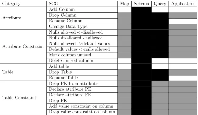
With the four categories of maintenance defined (Map, Schema, Query, Application), the next step is to define which of these categories is applicable to each potential SCO. Each SCO by definition modifies the database schema, so the Schema category is automatically included in each maintenance calculation. Additionally, each SCO will require a subset of the other three categories to be included in the calculation, because each SCO varies in its impact on the components of the IS.
Table 2.2 shows the exact mapping of each SCO to the categories of maintenance that must be evaluated for it. A black box indicates that the category must always be evaluated for the SCO, whereas a gray box indicates that the category must be evaluated only if the variables on which the SCO operates are mapped in the map table. To demonstrate explicitly how and why the mappings in Table 2.2 work, we go through a few examples of schema changes.
Example: Adding Columns
Adding new columns to the database schema is the simplest example of a schema change. Such a change introduces brand new columns rather than modifying or deleting existing ones, and it is therefore impossible for the columns to be present
in any existing query, application code, or the map table. As a result, the only maintenance to be calculated is the schema category.
Example: Dropping Columns
Compared to adding columns, dropping columns is a much more disruptive change. Deleting a column in the database will affect all queries that access it, as well as any application variable into which the column is mapped. Therefore, dropping a column requires all four categories to be computed.
Example: Renaming Columns
Renaming a column in the database naturally affects the queries that access it, as well as the map table, since the mapping must be updated to reflect the new name. However, the application code itself shouldn’t be affected - the application variables may stay untouched as long as the queries are appropriately updated to map the new column name into them.
Example: Dropping Tables
Calculating the maintenance of dropping a table is equivalent to the sum of the main-tenance of dropping each individual column of the table. Therefore, the categories needed are the same as that of dropping columns, i.e. all four categories.
2.2.5
Summary
With the SCO mapping established, the process of quantifying the maintenance cost of a particular schema change is now well defined, albeit at a high level. The ap-proaches outlined in this chapter are put into practical use in Chapter 3, where the implementation of the Co-Evolution Assistant tool is discussed in detail. As discussed in this chapter, the majority of the difficulty of the implementation lies in the com-plexities of application maintenance computation. Devising an algorithm to correctly compute application maintenance is a main focus of the implementation.
Category SCO Map Schema Query Application Add Column
Drop Column Rename Column Attribute
Change Data Type
Nulls allowed ->disallowed Nulls disallowed ->allowed Nulls allowed ->default values Default values ->nulls allowed Mark column unused
Attribute Constraint
Delete unused column Add table
Drop Table Table
Rename Table
Drop PK from attribute Declare attribute PK Declare attribute FK Drop FK
Add value constraint on column Table Constraint
Drop value constraint on column
Chapter 3
Implementation
In Chapter 2, we laid out the high-level proposal of the Co-Evolution Assistant: a tool for IS maintainers that provides an analytical breakdown of the impact of any proposed schema change. In this chapter, we discuss the implementation details of how we created a tool to carry out such an analysis.
3.1
Architecture Overview
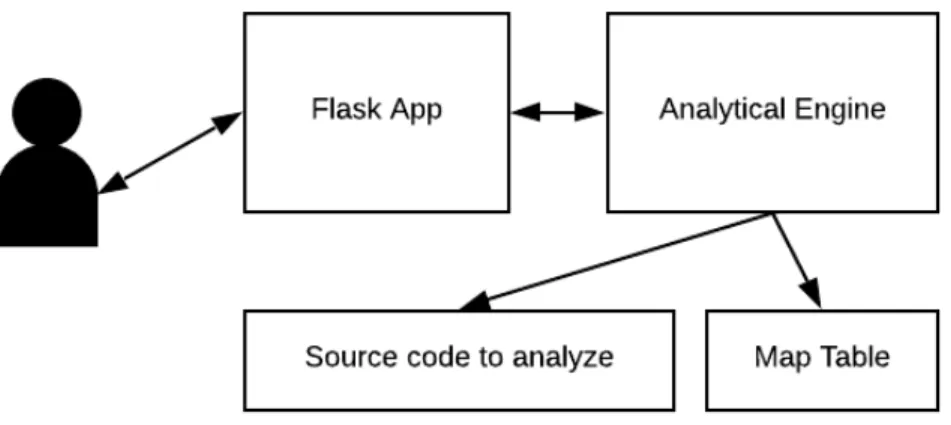
Figure 3-1 shows the basic architecture of the Co-Evolution Assistant. It is imple-mented as a lightweight web app, built on the Flask framework. At a high level, users interact with the app, sending schema change requests through to the back end. The app talks to the analytical engine, written in Python, which then is responsible for the heavy computation of the analysis. To carry this analysis out, the engine must have access to both the full source code as well as the map table.
3.2
The Analytical Engine
The bulk of the Co-Evolution Assistant’s heavy lifting lies in the analytical engine, whose job is to analyze a given IS codebase. To this end, the engine was designed accommodate any general system. However, in practice, it is necessary to make some constraints to the system, as designing a tool that works perfectly with any arbitrary
Figure 3-1: Architecture overview of the Co-Evolution Assistant
IS would be virtually impossible (and out of the scope of this project).
3.2.1
IS Code Constraints
Here we lay out the restrictions that we impose on application code of the IS to be analyzed. These restrictions are separate from the criteria described in section 2.1.1: while those are general structural criteria for the type of IS to which the Co-Evolution Assistant is applicable, the following are specific guidelines pertaining only to the application code on which the IS is built.
1. The most restrictive criterion is that the IS must be written in Java. This was a consideration made from the start of the project, with the potential of supporting more languages in the future. Targeting a single programming language was required, due to the way the analysis of the codebase is carried out with static analysis (discussed in detail in 3.4).
2. The schema structure and database queries must be defined in their own sep-arate files. The analysis code to quantify impact will need to be directed to specific files, in order to calculate correct metrics pertaining only to these cat-egories.
3.2.2
Creating the Map Table
As discussed in 2.2.2, the map table’s job is to link database variables to their coun-terpart variable in the application code. This mapping is critical to determining the impact of a schema change, as it enables immediate identification of which application variables are affected by a certain SCO.
In our implementation, the map table is created manually, as a comma-separated value (CSV) file. This requires examination of each query used by the application code. For each one, a row in the map table must be made, linking the database column being accessed to the application variable that it populates. As seen in the example in Table 2.1, some metadata is also included about the mapping - in particular, the versions over which the mapping is applicable, as well as the application class in which it appears. Thus, if the user wishes to analyze multiple versions of the codebase, the map table must be updated to include information relevant to each one.
In this version of the Co-Evolution Assistant we create the map table manually, though it is theoretically possible to programmatically generate the table instead. To do so requires parsing of the connector code that links application variables to their database counterparts, for each stored version of the source code repository. This can be done by examining each query present in the code, and furthermore inspecting the ways in which the results of the query are mapped into application variables. We leave this possibility open for future versions of the Co-Evolution Assistant. However, for the present version, we do not yet support automatic map table creation, for reasons mainly related to generalizability. While it may be straightforward to implement an automatic map table generator for a specific IS’s query patterns, it is much more difficult to build a generator that works for any IS. There is no set way in which the queries are constructed, executed, and the results applied to the application, so an all-purpose solution would have to be robust to every possibility. Being generally applicable is a main goal of the Co-Evolution Assistant, and so for this version of the Co-Evolution Assistant, we choose to create map tables manually.
3.2.3
Static vs. Dynamic Analysis
As discussed in Chapter 2, the computation of all maintenance categories except ap-plication is straightforward. However, for apap-plication maintenance, a substantially more complex computation is required. It was briefly mentioned in Section 2.2.3 that a static analysis approach is preferred to a dynamic one when calculating this par-ticular metric. The reason is that of general compatibility: having the Co-Evolution Assistant be usable on any codebase, with little setup, is one of the main goals of the project. Dynamic analysis impedes the general compatibility of the tool, since it inherently requires some setup work that is specific to the IS on which it is operating. There do exist dynamic analysis tools via which some version of the analysis we want could be done, such as Soot or ANTLR, for Java [3][4]. However, such analysis tools are generally meant to be run dynamically on top of compiled and/or instrumented code. This can severely impact the Co-Evolution Assistant’s goal of working quickly on any IS. While each IS to be analyzed will be required to share certain similar properties, they will differ in many other respects, such as overall structure, code layout and semantics, and compilation process. As a result, it would be virtually impossible to design a tool capable of dynamically instrumenting code while at the same time remaining applicable to a general system. For this reason, for calculating application maintenance, we choose to employ a static analysis solution instead of a dynamic one.
3.2.4
Engine State
The state maintained by the engine is largely static, and initialized on creation. It consists of four main categories:
1. File locations: the file paths of the code to be analyzed. This includes loca-tions of the application code, the schema and query declaration files, and the map table file.
2. Versioning information: The unique identifier of the version of the IS to be analyzed. Typically a Git commit hash.
3. Map table: While the map table is stored persistently on disk as a file, in the interest of efficiency during analysis, the engine reads the file into an in-memory data structure, albeit at the cost of memory space. The map table is generally of a reasonable size to be held in memory.
4. SCO mappings: The engine maintains the mapping shown in Table 2.2 in order to properly compute the impact of schema changes requested by the user.
3.2.5
Strategies for Computing Maintenance
The main task of the engine is to compute maintenance estimates for the schema changes that it is given. A high level overview of the process is outlined in section 2.2; here, we go over the lower-level implementation details. In summary, the proposed schema change is broken down into its constituent SCOs, which are individually computed and summed together to make the total estimate. Each SCO’s impact is computed based on the applicable categories, according to Table 2.2. A summary of the implementation strategy for each category is described below.
Map Maintenance
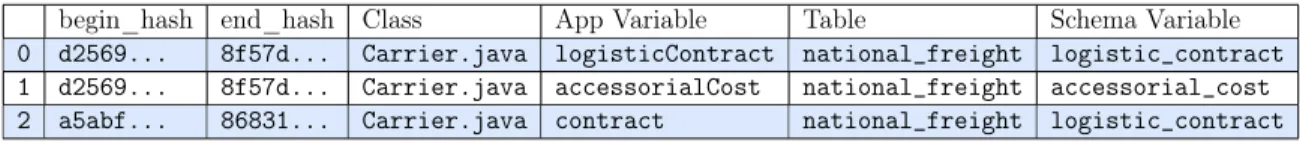
Map maintenance is straightforward to compute. Intuitively, the impact of modifying a specific variable is simply the number of entries that pertain to that variable, if it is mapped in the table. Specifically, given a schema change acting on some schema variable 𝑠, all map table entries linking 𝑠 to an application variable must be counted. Since the map table is stored on disk as a CSV file, all such affected entries can be found with a simple linear scan of the rows. As an example, Table 3.1 (same as the example excerpt of a map table in Table 2.1) shows the rows that would be included in a map maintenance calculation on the schema variable logistic_contract. In this case, since logistic_contract is mapped by two rows, the map maintenance result would be 2.
begin_hash end_hash Class App Variable Table Schema Variable 0 d2569... 8f57d... Carrier.java logisticContract national_freight logistic_contract 1 d2569... 8f57d... Carrier.java accessorialCost national_freight accessorial_cost 2 a5abf... 86831... Carrier.java contract national_freight logistic_contract
Table 3.1: Rows included in an example map maintenance computation on logistic_contract
Schema and Query Maintenance
Computing schema and query maintenance is also straightforward to compute. By definition, a change to a schema variable 𝑠 requires modifying the schema declaration files. Similarly, any query operating on 𝑠 will be impacted, and must also be modified. Since the engine state stores the file locations of both the schema and query files on creation, the maintenance can be computed in a similar way to the map table: scan the respective file, and count the instances of 𝑠, the affected variable.
As an example of schema maintenance, consider the schema is shown in Listing 3.1. A proposed SCO to drop a column, e.g. LOGISTIC_CONTRACT, would equate to removing line 9 in the schema. Given the name of the column to drop, finding its corresponding line in the schema definition requires just a simple linear scan of the schema. 1 C R E A T E T A B L E " S A L E S _ A C O M _ A D M I N "." N A T I O N A L _ F R E I G H T " ( 2 " I N I T I A L _ W E I G H T " N U M B E R NULL, 3 " F I N A L _ W E I G H T " N U M B E R NULL, 4 " P R I C E " N U M B E R NULL, 5 " M U L T I P L I E R _ T Y P E " V A R C H A R 2( 2 0 ) NULL, 6 " P O S T A L _ C O D E _ S T A R T " N U M B E R NULL, 7 " P O S T A L _ C O D E _ E N D " N U M B E R NULL, 8 " C A R R I E R _ C N P J " V A R C H A R 2( 2 0 ) NULL, 9 " L O G I S T I C _ C O N T R A C T " V A R C H A R 2( 2 0 ) NULL, 10 " D A Y S " N U M B E R NULL, 11 " A C C E S S O R I A L _ C O S T " N U M B E R NULL, 12 " S U F R A M A " C H A R(1) NULL, 13 " W A R E H O U S E _ I D " N U M B E R N U L L 14 )
Application Maintenance
Application maintenance is by far the most complex computation to execute, and constitutes the bulk of the engine’s heavy lifting. Section 2.2.3 outlines the challenges of the computation. The effect of modifying a schema variable 𝑠 that maps into an application variable 𝑎 depends heavily on how 𝑎 is used in the application code. For example, 𝑎’s value could be propagated to other variables, classes, or modules; used to guide the code’s control flow; etc. The analytical engine’s job is to trace the path of 𝑎 through the codebase, starting at the point at which it is populated from the database. Once these paths are found, 𝑎’s impact can be quantified by the number and length of its paths of influence. The difficulty of this computation lies in finding the variable’s paths, and the algorithm used is described in detail in the following section.
3.3
Tracing Application Variables
Tracing the paths taken by application variables through the code is a complex task. In our case, statically analyzing a codebase involves writing code to inspect the con-tents of the codebase’s source code files. Specifically, since we are executing the analysis to compute application maintenance, our analysis will scan the source code to quantify the impact of a particular application variable. This amounts to tracing the variable to all the places in the code that are in some way affected by its value.
Intuitively, the problem of tracing a certain variable 𝑎’s effect throughout a pro-gram boils down to a simple concept: follow 𝑎 to all the lines of code in which it is used. For each of those lines, 𝑎 may be used to influence the values of new variables, via assignment or otherwise. Those new variables will further influence other parts of the code, propagating the influence of 𝑎 further. This basic idea will guide the creation of an algorithm to correctly analyze the influence of a given variable.
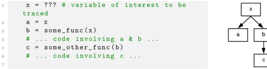
1 x = ??? # v a r i a b l e of i n t e r e s t to be t r a c e d 2 a = x 3 b = s o m e _ f u n c ( x ) 4 # ... c o d e i n v o l v i n g a & b ... 5 c = s o m e _ o t h e r _ f u n c ( b ) 6 # ... c o d e i n v o l v i n g c ... 7
Figure 3-2: A simple example of application variable tracing
3.3.1
A Simple First Approach
With the basic idea in mind, we can take a first stab at an algorithm to find the effect of a specific variable 𝑎 through the code. We will maintain a set 𝑆 of variables that must be traced, which initially contains only 𝑎. As we find more variables influenced by 𝑎, they will be added to the set, and traced as well. For each variable 𝑠 in the set, first, as mentioned previously, find all instances of 𝑠 being used in the code. If it is on the right hand side of an assignment statement, trace whichever new variable 𝑏 is on the left hand side as well, since 𝑠’s value has now been propagated to 𝑏. The same tracing process must then be repeated on each new variable added to this set of variables that have been affected.
Figure 3-2 illustrates a simple example of a program in which the value of a variable x influences the subsequent values of variables a, b, and c. We step through the program line by line to follow x’s path. On line 2, a is simply assigned to the value of x, indicating that we must now keep track of a as well as x. Then, in line 3, the result of a function call with x as an argument is assigned to the variable b, adding b to our set of variables of which to keep track. Finally, in line 5, b is passed to a function call that results in c. This flow of propagation can be represented as a tree, with x as the source. Since a and b’s values are assigned as direct functions of x, they are x’s immediate children. Similarly, c is the child of b, since its value is a direct function of b. When tracing a variable’s effect in the code, at a high level, the goal of the process is to find all such paths from the root to leaf, and expose them to the user.
1 c l a s s E x a m p l e () :
2 def _ _ i n i t _ _ ( self , var ) :
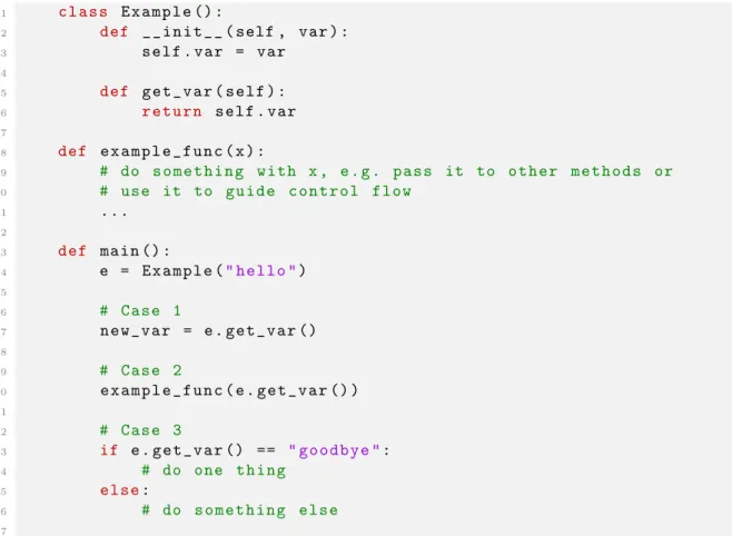
3 s e l f . var = var 4 5 def g e t _ v a r ( s e l f ) : 6 r e t u r n s e lf . var 7 8 def e x a m p l e _ f u n c ( x ) : 9 # do s o m e t h i n g w i t h x , e . g . p a ss it to o t h e r m e t h o d s or 10 # use it to g u i d e c o n t r o l f l o w 11 ... 12 13 def m a i n () : 14 e = E x a m p l e (" h e l l o ") 15 16 # C a s e 1 17 n e w _ v a r = e . g e t _ v a r () 18 19 # C a s e 2 20 e x a m p l e _ f u n c ( e . g e t _ v a r () ) 21 22 # C a s e 3 23 if e . g e t _ v a r () == " g o o d b y e ": 24 # do one t h i n g 25 e l s e: 26 # do s o m e t h i n g e l s e 27
Figure 3-3: Examples highlighting failure points of the simple approach
3.3.2
Weakness of Simple Approach
Tracing based solely on assignment statements is an extremely bare-bones approach that has the correct high-level idea, but disregards the nuances of the way data flows through programs, and would inevitably yield incomplete results if implemented as-is. To illustrate a few cases of variable propagation that the algorithm would not pick up on, consider the code shown in Figure 3-3. Let’s say that the variable of interest is the instance variable var of the Example class, which has a method get_var to expose var. The driver code in main creates a new instance of the Example class, passing it the string "hello" to store as var. The following are some examples of cases in which the value of var is used to influence the program, without any assignment statements.
Case 1
On line 17, we have a very basic case of variable propagation that would pass un-noticed by the simple assignment-based approach. We assign new_var to the value returned by Example.get_var, which is in this case the exact variable we are tracing. As such, we should be interested in tracing new_var in order to see to where it prop-agates the value of var. Line 17 is an assignment statement, but since the access to var is hidden behind a function call (Example.get_var) rather than directly access-ing the variable, this propagation would not be recognized by the simple algorithm. As a result, any subsequent usage of new_var would, incorrectly, not be reported.
Case 2
On line 20, example_func is called, and is passed as an argument the result of get_var. example_func presumably uses the argument that it is passed in a mean-ingful way, which is precisely the kind of usage that we are interested in when tracing var. However, since line 17 did not involve any assignment, the simple approach is un-able to detect that var’s value is being passed to (and used in) example_func. Thus, the assignment-based approach breaks down in instances where variables’ values are propagated via function calls.
Case 3
On line 23-26, we have an example of var being used to guide the program’s control flow. The conditional statement chooses a block of code to execute based on the value of e.get_var(), i.e. var. This is certainly a case of code behavior being influenced by var, but since it involves no assignments, it would not be detected by the simple approach as a case of propagation. This is yet another case in which the assignment-based approach is insufficient for discovering the full influence of a variable.
Learnings
The previous three cases illustrate the difficulties that lie in writing a program that accurately calculates application maintenance. It is clear that the simple approach falls short of discovering the full influence that a given variable has on the codebase. In particular, we identify the cases that a correct algorithm must handle:
∙ Propagation via return statement: In Case 1, var is returned from get_var. As a function that directly exposes var, any instance of get_var being called should then be treated equivalently to var itself. In general, when a function returns a variable that is being traced, any calls to that function should be treated like a traced variable.
∙ Propagation via function call: In Case 2, var is passed as an argument to a function. The way that var is used within that function is therefore of interest, and should be inspected for further propagation. A correct algorithm must therefore be able to detect when a variable being traced is passed as an argument to function calls. Furthermore, it must step inside that function, and continue to trace the argument.
∙ Influence on program control flow: In Case 3, the value of var was used to guide the logical flow of the program. The tracing algorithm should be able to recognize and point out these cases of influence.
3.4
Variable Tracing Algorithm
As we saw in the previous section, there are numerous shortcomings of the simple, assignment-based approach for tracing variables through the code. We then laid out several requirements that a proper algorithm must fulfill in order to return complete, correct results. In this section, we describe in detail the full algorithm that was written to compute application maintenance while adhering to the aforementioned constraints.
Algorithm Phases
The algorithm is broken into three main phases:
1. Pre-processing: First, a representation of the codebase is constructed in-memory. This pre-processing step converts each bare source code file into a more workable object-oriented representation, on which operations can be con-veniently performed.
2. Building relationships: Next, data structures representing relationships be-tween function calls made by the program are built up. As we saw in Sec-tion 3.3.2, funcSec-tion calls are an important mechanism for propagating variables through the code. In these structures, we store information that directly con-nects each function to functions that call it, or callers. This information is then used in the third phase of the algorithm.
3. Traversal: Once the proper state has been set up, the actual traversal of the code base for the paths of influence for a given variable must be executed. This phase yields the final result, which is a number representing the total calculated application maintenance.
These phases are described in detail in the following sections.
3.4.1
Source code pre-processing
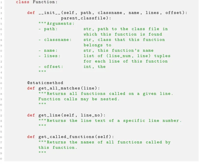
In the second phase, we need to relate each function to its caller functions. Before doing so, it is useful to have an in-memory object representation of each function, in order to quickly access metadata about it (e.g. name, class, number of lines). Thus, in this pre-processing phase, we create a map of function name to its corresponding Function object. A simplified API of the Function class is shown in Figure 3-4.
The most important method of the class is Function.get_called_functions. This method returns the names of all the functions called from within a particular function. As such, it is used heavily in the second phase of the algorithm, when the relationships between functions are built up.
1 c l a s s F u n c t i o n : 2
3 def _ _ i n i t _ _ ( self , path , c l a s s n a m e , name , lines , o f f s e t ) :
4 p a r e n t _ c l a s s f i l e ) : 5 """ A r g u m e n t s : 6 - p a t h : str , p a t h to the c l a s s f i l e in 7 w h i c h t h i s f u n c t i o n is f o u n d 8 - c l a s s n a m e : str , c l a s s t h a t t h i s f u n c t i o n 9 b e l o n g s to 10 - n a m e : str , t h i s f u n c t i o n ’ s n a m e 11 - l i n e s : l i s t of ( l i n e _ n um , l i n e ) t u p l e s 12 for e a c h l i n e of t h i s f u n c t i o n 13 - o f f s e t : int , the 14 """ 15 16 @ s t a t i c m e t h o d 17 def g e t _ a l l _ m a t c h e s ( l i n e ) : 18 """ R e t u r n s all f u n c t i o n s c a l l e d on a g i v e n l i n e . 19 F u n c t i o n c a l l s may be n e s t e d . 20 """ 21 22 def g e t _ l i n e ( self , l i n e _ n o ) : 23 """ R e t u r n s the l i n e t e x t of a s p e c i f i c l i n e n u m b e r . 24 """ 25 26 def g e t _ c a l l e d _ f u n c t i o n s ( s e l f ) : 27 """ R e t u r n s the n a m e s of all f u n c t i o n s c a l l e d by 28 t h i s f u n c t i o n . 29 """ 30
In order to create a Function object for each function in the code, each source code file is individually parsed. Since the code is written in Java, the lines pertaining to each method of each class can be extracted by performing a linear scan while keeping count of { and } characters, which delimit the beginning and end of each method. Then, the lines are used to create a new Function object, which is then stored in a map from function_name : Function. This map is an integral part of the second phase, in which function relationships are built up.
3.4.2
Building relationships
In the next stage of the algorithm, we examine the ways in which function calls prop-agate data through the program. We previously saw in Section 3.3.2 how functions can be used to expose the variable being traced to a caller function (Case 1), or al-ternatively, take in the variable being traced as an argument. In general, all types of function calls encountered when scanning a program can be generalized into one of two cases: upwards or downwards propagation. Intuitively, the "direction" asso-ciated with each type of propagation refers to whether the data being propagated is being returned "upwards" to the caller, or being passed "downwards" to a function call. It is necessary to distinguish between types ("directions") of function calls in order to properly trace data flowing through the program.
Upwards Propagation
For a particular variable of interest v, a function call that propagates v upwards simply returns a variable whose value depends in some way on v. In its simplest form, this is just a function that returns v itself. More complex examples are endless, but include objects instantiated with v as a parameter, data structures containing v, etc.
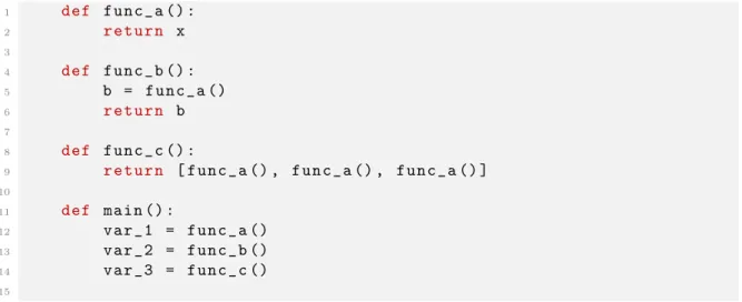
A few examples of upwards propagation are shown in Figure 3-5, with var_1, var_2, and var_3 as products of the propagation. The variable being traced in these examples is some global variable x. The simplest example is func_a, which just
1 def f u n c _ a () : 2 r e t u r n x 3 4 def f u n c _ b () : 5 b = f u n c _ a () 6 r e t u r n b 7 8 def f u n c _ c () : 9 r e t u r n [ f u n c _ a () , f u n c _ a () , f u n c _ a () ] 10 11 def m a i n () : 12 v a r _ 1 = f u n c _ a () 13 v a r _ 2 = f u n c _ b () 14 v a r _ 3 = f u n c _ c () 15
Figure 3-5: Examples of upwards propagation via function calls
returns x itself. func_b is just a wrapper around func_a, and ultimately returns the same value x. Lastly, func_c returns a list, with values populated from func_a. Since all three functions return values that either are x or directly depend on the value of x, it can be said that all three propagate their return values upwards to the caller function (main).
Downwards Propagation
Conversely, for a particular variable of interest v, a function call that propagates v downwards will do the opposite of upwards propagation: it will take v as an argument, and use it to guide downstream logic or variables. In short, no value dependent on x will be propagated back to the caller to be used.
In Figure 3-6, we can see a typical example of downwards propagation. In the driver code, in main, var_1 is propagated downwards as an argument to Example.add_var, which returns nothing. Rather than returning some value, Example.add_var uses its argument to influence or modify data further down the chain of calls. Specifically, in the figure, it appends the argument var to its internal list.
1 c l a s s E x a m p l e () :
2 def _ _ i n i t _ _ ( s e lf ) :
3 s e l f . v a l u e s = []
4
5 def a d d _ v a r ( self , arg ) :
6 s e l f . v a l u e s . a p p e n d ( arg ) 7 8 def f u n c _ a () : 9 r e t u r n x 10 11 def m a i n () : 12 e = E x a m p l e () 13 v a r _ 1 = f u n c _ a () 14 e . a d d _ v a r ( v a r _ 1 ) 15
Figure 3-6: Examples of downwards propagation via function calls
Categorizing Function Calls
With the two categories of function propagation in mind, we are now equipped to categorize the function calls present in the program. Thus, we scan each function found in the first phase of the algorithm for function calls within its body. To do so, we simply use the method Function.get_called_functions. When called on a function f, this method returns to us a list of all the functions called from within the body of f. The functions are returned as a list of tuples of the form (called_function_name, upwards), where upwards is a boolean, representing the direction of propagation of that particular function call.
The mapping we build during this step is of the form function_name : { set of all functions that call this function}. By mapping each function to the functions that invoke it, in the traversal step, we will easily be able to walk propa-gation paths backwards from a source. To build this mapping, we iterate over each function F. For every function f called from within F, F is the caller, and f is the callee. Thus, F is added to the set of functions attached to key f.
3.4.3
Traversal
The final phase of the algorithm is the traversal of propagation paths. Having built up the necessary data structures in the first two phases, the traversal is relatively simple. Given a target variable v, we will treat it as our starting point, and find all the code paths stemming from this source.
Finding source functions
The data structures we built up in the first two stages of the algorithm represent the relationships between function calls in the program. However, in practice, we will be given a certain variable to trace, not a source function. Thus, before traversing any of the data structures, we must first determine the source function(s) that expose the variable of interest. Once those source functions are determined, we will traverse backwards from each one.
The value of the variable to be traced, v, is always mapped in from the database. Commonly, v is an instance variable on a class, and is exclusively exposed to the rest of the code via a getter method, which simply returns a safely accessible version of the variable. In this case, that getter method would be the single source function for v. In other cases, v may be exposed from multiple source functions. Either way, the traversal always begins from a specific set of one or more source functions. Finding such source functions is a matter of finding functions that directly reference and/or expose v, which can be accomplished via individually scanning each function for its variable usage.
Tracing paths
Once the source functions are identified, tracing is executed for each one. In this way, all possible paths that the variable takes through the code will be found. Pseudocode of the recursive traversal algorithm is shown in Figure 3-7. At a high level, given a start function, we branch outwards to follow each subsequent function call that propagates the return value to other places in the code.
1 def t r a v e r s e ( s t a r t _ f u n c , s t a r t _ l i n e _ n u m ) : 2 p a t h s = {} 3 4 if s t a r t not c a l l e d by any f u n c t i o n : 5 p a t h s [( s t a r t _ f u n c , s t a r t _ l i n e _ n u m ] = {} 6 r e t u r n p a t h s 7 8 l i n k s = all f u n c t i o n s t h a t c a l l s t a r t _ f u n c 9 10 for e a c h c h i l d l i n k L in l i n k s : 11 c h i l d _ k e y = ( L . name , L . l i n e _ n u m ) 12 upwards , p r o p a g a t o r = L . upwards , L . p r o p a g a t o r 13 14 if u p w a r d s : 15 c h i l d _ p a t h s = t r a v e r s e (* c h i l d _ k e y ) 16 p a t h s [ c h i l d _ k e y ] = c h i l d _ p a t h s 17 e l s e : 18 f i n a l _ l i n e _ n u m = p r o p a g a t o r _ f n . f i r s t _ l i n e _ n u m 19 f i n a l _ l i n k = ( p r o p a g a t o r , f i n a l _ l i n e _ n u m ) 20 p r o p a g a t e d _ p a t h s = { f i n a l _ l i n k : {} } 21 p a t h s [ c h i l d _ k e y ] = p r o p a g a t e d _ p a t h s 22 23 r e t u r n p a t h s 24
Figure 3-7: Pseudocode of the traversal algorithm
The algorithm is recursive, and the result is a nested series of maps representing the paths that the variable takes through the code. At each step, we branch out one step from the start function passed in. Since we have constructed a mapping of each function to the functions that call (i.e. propagate) it, we can find the propagator functions instantly (line 8). Next, for each propagator function f, there are two cases for the direction of propagation: upwards or downwards.
∙ Upwards (lines 14-16): In the case that the f propagates the variable upwards, the same process is recursively applied on this propagator function. As long as the propagation is in the "upwards" direction, the algorithm will continue to recursively step backwards in this manner, up the chain of function calls. We add the result of the recursive call to the map.
∙ Downwards (lines 18-21): If f propagates downwards, there should be no recursive call, because the propagation flows into the called function, rather
than back up a chain of function calls. So, we step into the function call and inspect all usages of the variable to be traced. To indicate this, we add one final link to the map, consisting of f’s information.
The final result of a call to the traversal function is a series of nested maps, with each subsequent layer of nesting representing one step on the variable’s path. This path representation is in a convenient format to be transformed into a digestible display for the user.
3.5
The Interface
Ultimately, the goal of the Co-Evolution Assistant is to be a developer tool. With this in mind, it is ideal to provide an easy-to-interpret interface to users. The alternative would be to have users run the bare code, and interpret the results manually. This invites problems of general compatibility, and additionally requires the developer to understand a substantial portion of the code in order to both run it and correctly parse the results.
To avoid such overhead for developers, we created a lightweight web application, which wraps the code for the analytical engine (Section 3.2). It provides a simple interface for users to enter parameters of any proposed schema change, and reports back the maintenance estimates for each of the four categories mentioned in 2.2.3.
3.5.1
User input
The input parameters available to the user are as follows:
∙ Source code paths: specify where the source code to be analyzed is located. ∙ Map table path: the location of the map table CSV file.
∙ Repository version: the Git commit hash of the version of the repository to be analyzed.
Figure 3-8: Sample result table for a proposed schema change
3.5.2
Result interface
The result of submitting a schema change is presented to the user in a digest, broken down into the four maintenance categories: schema, query, application, and map. An example result table, obtained from running the Co-Evolution Assistant on a real system, is shown in Figure 3-8. There is an additional column present, simple_add, which is responsible for adding a small, constant amount of maintenance to the es-timate in the case of creation of a new table or column. In this example, neither of those cases are applicable. Additionally, the table groups each SCO by the database table upon which it acts.
Two schema change operators were entered to produce this table: one DROP_TABLE operation on table NATIONAL_FREIGHT, and one DROP_COLUMN operation on table B2W_CKT_FR_DAYS. In the figure, the results table is fully expanded, to show the details for each SCO. For schema, query, and map maintenance, the reported infor-mation is straightforward: a file name, and a link to jump to each affected line in the code. For application maintenance, however, the result is not so simple. As we saw
Figure 3-9: Example tree-based view of a variable’s paths through the code
in Section 3.4, the result of tracing a variable through the code to compute its appli-cation maintenance results in one or more paths, which represent the variable’s steps through function calls. To display this efficiently, we designed a secondary interface to display these paths.
Application Maintenance Summary
The overall result table links into the secondary application maintenance summary page. This page displays every path that the variable takes through the code, in both a combined tree-like format and an individual format. An sample nested tree view is shown in Figure 3-9, for the variable logisticContract. The root of the paths is the outermost function call, which in this case is getLogisticContract. This makes
sense, as all paths should stem from the function that exposes logisticContract in the first place. One layer in to the tree, we can see that the tree branches five ways -indicating that logisticContract is accessed via getLogisticContract five times throughout the code. In the second branch, as shown in the figure, by expanding the code snippet, we can see that the path ends at the function setLogisticContract.
Chapter 4
Discussion
In the first three chapters, we laid out the motivation for and implementation details of the Co-Evolution Assistant. In this chapter, we put it to use on a real-world use case. To do so, we use the Co-Evolution Assistant to analyze proposed schema changes on B2W’s Checkout, a large industrial e-commerce platform.
4.1
B2W Checkout
The application to which we apply the Co-Evolution Asssistant, Checkout, is a large, multi-modular system built by B2W, the largest South American online retailer [5]. It is a platform for handling the end-to-end customer experience as they shop online.
4.1.1
Characteristics
The Checkout codebase is large, and is comprised of more than 60 individual modules. These include Order, Customer, Freight (order delivery), Inventory, Promotion, Installment, Payment, Cart, and Account. Of these modules, the modules Order, Customer, and Freight were the most important, and were iterated upon most heav-ily by the engineers over the lifetime of Checkout.
The Checkout application is written in Java, and uses the Java Database Connec-tivity (JDBC) Connector to connect to more than 40 Oracle database tables. Freight
used the most database tables of any individual module by far, at 13. Since it is the most complex and therefore best illustrate the full functionality of the Co-Evolution Assistant, we use it for the examples in this chapter.
4.1.2
Applicability of Co-Evolution
B2W’s Checkout was an ideal candidate on which to validate the Co-Evolution As-sistant, due to its fully-fledged development history and varied evolution patterns (in addition to meeting the criteria outlined in 2.1.1 and 3.2.1). Over the course of its 74-month development period [5], it underwent significant structural overhaul, due in some cases to precisely the types of schema changes that the Co-Evolution Assistant is designed to help with.
4.2
Results
Here, we present the results of applying the Co-Evolution Assistant to the Freight module of Checkout. While it is not possible to anticipate all future schema changes to a system, we can still explore and analyze realistic schema changes to the codebase. By doing so, we highlight how the Co-Evolution Assistant works in a practical setting.
4.2.1
Dropping Tables
In practice, the need for restructuring data in response to a changing business con-dition is common. In one particular case, data in a single table must split out into multiple tables. In terms of SCOs, this amounts to a drop table operation, accom-panied by adding one or more tables, into which the data will be shifted. While we cannot anticipate the schema structure of new tables, we can analyze the impact caused by dropping the original table.
In general, these drop table SCOs are the most disruptive to the system, as they affect variables in bulk, and require careful handling on the application side to keep it safely intact. Referring to Table 2.2, we can see that a drop table operation requires
all four maintenance categories to be calculated. In terms of implementation, com-puting the maintenance for dropping a table is effectively the same as comcom-puting the maintenance for dropping each of the table’s constituent columns, and summing the results for each one. This is precisely what the Co-Evolution Assistant does: given a table to drop, it finds the maintenance associated with dropping each column in the table, and reports back the sum total maintenance.
4.2.2
Walking through an Example Schema Change
In this example, we walk through the theoretical process of dropping one of the Freight module’s main tables, B2W_CKT_FR_DAYS. We examine each maintenance metric individually, and validate that the Co-Evolution Assistant satisfactorily and thoroughly evaluates the impact of dropping the table.
Schema Maintenance 1 C R E A T E T A B L E " S A L E S _ B 2 W _ W L _ A P P "." B 2 W _ C K T _ F R _ D A Y S " ( 2 R E G I O N _ C O D E V A R C H A R 2( 2 0 ) , 3 I N I T I A L _ W E I G H T NUMBER, 4 F I N A L _ W E I G H T NUMBER, 5 W A R E H O U S E _ I D NUMBER, 6 C O N T R A C T _ T Y P E V A R C H A R 2(5) , 7 P R O M O T I O N _ T Y P E V A R C H A R 2( 2 0 ) , 8 P E R I O D C H A R(1) , 9 L O G I S T I C _ C O N T R A C T V A R C H A R 2(2 0 ) , 10 D A Y S NUMBER, 11 P R I C E NUMBER, 12 S P E C I A L _ D E L I V E R Y C H A R(1 B Y T E ) , 13 H R _ C O R T E N U M B E R(2) 14 )
Listing 4.1: B2W_CKT_FR_DAYS schema
The schema of B2W_CKT_FR_DAYS is reproduced in Listing 4.1. Dropping the table requires deleting the entire schema. As discussed before, the Co-Evolution Assistant
will compute schema maintenance for each column individually, then combine the results to represent the effect of dropping the entire table. In this case, the tool will simply search for each column name in the schema individually, and report each one back. In this way, the entire schema will be taken into account.
Query Maintenance
Similarly, for query maintenance, the basic idea is to search for each table variable in all query definitions. By doing so, each query affected by the table will be highlighted. In the case of B2W_CKT_FR_DAYS, there is one main query that pulls in data from the database to the application side, represented (in a truncated form) in Listing 4.2. In particular, it pulls the columns warehouse_id, days, price, logistic_contract, and special_delivery into the application.
1 S E L E C T D I S T I N C T D . c o n t r a c t _ t y p e AS C O N T R A C T _ T Y P E , 2 D . w a r e h o u s e _ i d AS W A R E H O U S E , 3 P . v l _ f r e i g h t AS S A L E _ P R I C E , 4 D . d a y s AS DAYS , 5 D . p r i c e AS PRICE , 6 D . l o g i s t i c _ c o n t r a c t AS L O G I S T I C _ C O N T R A C T , 7 D . s p e c i a l _ d e l i v e r y as S P E C I A L 8 F R O M B 2 W _ C K T _ F R _ D A Y S D 9 I N N E R J O I N B 2 W _ C K T _ F R _ R E G I O N R ON ... 10 L E F T J O I N B 2 W _ C K T _ F R _ P R I C E P ON ... 11 AND D . c o n t r a c t _ t y p e = P . c o n t r a c t _ t y p e 12 AND D . w a r e h o u s e _ i d = P . w a r e h o u s e _ i d 13 AND ? B E T W E E N P . i n i t i a l _ w e i g h t and P . f i n a l _ w e i g h t 14 W H E R E ? B E T W E E N R . p o s t a l _ c o d e _ s t a r t AND R . p o s t a l _ c o d e _ e n d 15 AND ? B E T W E E N D . i n i t i a l _ w e i g h t AND D . f i n a l _ w e i g h t 16 AND ... 17 O R D E R BY PRICE , D A Y S