HAL Id: hal-00704791
https://hal.archives-ouvertes.fr/hal-00704791
Submitted on 6 Jun 2012HAL is a multi-disciplinary open access
archive for the deposit and dissemination of sci-entific research documents, whether they are
pub-L’archive ouverte pluridisciplinaire HAL, est destinée au dépôt et à la diffusion de documents scientifiques de niveau recherche, publiés ou non,
radiated seismic intensity.
B. Taisne, Florent Brenguier, N.M. Shapiro, Valérie Ferrazzini
To cite this version:
B. Taisne, Florent Brenguier, N.M. Shapiro, Valérie Ferrazzini. Imaging the dynamics of magma propagation using radiated seismic intensity.. Geophysical Research Letters, American Geophysical Union, 2011, VOL. 38, pp.5 PP. �10.1029/2010GL046068�. �hal-00704791�
Imaging the dynamics of magma propagation using
1
radiated seismic intensity
2
B. Taisne,1 F. Brenguier,1,2 N.M. Shapiro,1 and V. Ferrazzini2,3
1Department of Seismology, Institut de
Physique du Globe de Paris, Sorbonne Paris Cit´e, CNRS (UMR7154), 1 rue Jussieu, 75238 Paris, cedex 5, France.
2Observatoire Volcanologique du Piton de
la Fournaise, Institut de Physique du Globe de Paris, Sorbonne Paris Cit´e, CNRS (UMR7154), 14RN3 - Km 27, 97418 La Plaine des Cafres, La R´eunion, France.
3G´eologie des syst`emes volcaniques,
Institut de Physique du Globe de Paris, Sorbonne Paris Cit´e, CNRS (UMR7154), 1 rue Jussieu, 75238 Paris, cedex 5, France.
At shallow depth beneath Earth’s surface, magma propagates through strongly 3
heterogeneous volcanic material. Inversion of buoyancy and/or solidification 4
have strong impacts on the dynamics of propagation without any change of 5
magma supply. In this paper, we study the spatial and time evolution of magma 6
intrusions using induced seismicity. We propose a new method based on es-7
timates of radiated seismic intensities recorded at different stations during 8
seismic swarms at Piton de la Fournaise volcano. By applying this method 9
to the January 2010 Piton de la Fournaise volcano eruption, we image com-10
plex dike propagation dynamics which strongly differ from a model of con-11
stant velocity dike propagation. We provide a new and fully automatic method 12
to image in real time the dynamics of dike propagation and to infer the po-13
sition of eruptive fissures. 14
1. Introduction
Eruption precursory activity associated to volcanic unrest is currently recorded at many 15
volcanological observatories around the world and mainly consists of seismicity and ground 16
deformation monitoring. During magma propagation to the near-surface, the vicinity of 17
the associated dike or sill is subjected to a large stress field perturbation [Rubin and 18
Gillard, 1998], that will concentrate most of the induced seismicity (seismic swarms). 19
Monitoring these seismic swarms is thus a potentially powerful technique to track magma 20
movements but is not used to its full potential for several reasons. During seismic swarms, 21
seismic events are difficult to separate, so that one may not use the efficient localization 22
methods that have been devised for single earthquakes. Only those events that are well 23
identified can be treated with current methods and a large part of the seismic signal is left 24
unused. Consequently, the interpretation of the data in term of the dynamics of magma 25
migration is difficult. Previously, few examples of migration of seismicity associated with 26
magma movement have been imaged by geophyscial means [Aoki et al., 1999; Hayashi and 27
Morita, 2003; Battaglia et al., 2005]. However, precise analysis of seismicity (localization, 28
magnitude) requires post-processing and is therefore difficult to perform in real time. 29
Here, we propose a simple but robust method to track magma movements using the 30
ratio at different seismic stations of the seismic intensities radiated by the surroundings of 31
the dike’s tip. We apply this method to the January 2010 eruption of Piton de la Fournaise 32
volcano (La R´eunion island). As a result, we observe a complex dike propagation dynamic 33
which strongly differs from a model of constant velocity dike propagation. We thus provide 34
a fully automatic and simple method to image in near-real time the dynamics of dike 35
propagation and to infer the position of eruptive fissures. 36
2. Method
Traditionally, seismic events are located using P or S wave travel time delays measured at different receivers. This approach finds its limits when it becomes difficult to measure accurate arrival times such as for example, during seismic swarms or in cases of low signal to noise ratio micro-seismicity. Here, we propose a method to automatically estimate the position at depth of a seismic source by using the differences in seismic amplitudes recorded at difference sensors. This approach relies on the attenuation of seismic waves along the source-receiver travel path. In order to avoid the detection of single P or S wave arrivals, we use an estimate of the average recorded seismic intensity over a time window much longer than the seismic wave travel time delays at different sensors (see section 3 for details). Following Battaglia and Aki [2003], we use a simple attenuation law that takes into account geometrical and intrensic but not scattering attenuation (equation 1).
Ii = Ao e−Bri rn i , (1) with, B = πf Qβ , (2)
where Ii is the seismic intensity recorded at receiver i, ri is the distance from the source,
37
Io is the source radiated seismic intensity, f is frequency, β is shear wave velocity and Q is
38
the quality factor for attenuation. The index n = 1 for body waves and n = 0.5 for surface 39
waves. For simplification we consider an isotropic medium with constant B. Because we 40
don’t know which type of wave (body or surface) dominates the intensity estimates, we 41
make no approximation about the value of n. In the next section we will investigate the 42
effect of n and Q. 43
To avoid the estimate of the seismic intensity at the source (Io), we choose to analyse the
ratios of seismic intensities between all sensors (equation 3) rather than the true seismic intensities at different sensors.
Ii Ij t = r t j rt i !n exph−B(rit− r t j) i . (3)
Assuming a migration such that rt+δt
i = rti + δi and rt+δtj = rjt+ δj, with δi and δj that
can be defined either positively or negatively depending on the relative direction of the source to the station:
Ii Ij t+δt = r t j + δj rt i+ δi !n exph−B(rti + δi− rjt− δj) i , (4)
by first order linearisation we obtain : Ii Ij t+δt = Ai Aj t" 1 + δj n rt j + B ! − δi n rt i + B !# . (5)
Equation 5 shows that only the migration of seismicity will affect the intensity ratio and 44
not the change of radiated seismic intensity at the source which does not appear in the 45
final equation. The only exception is if the motion occurs within the plane perpendicular 46
to the middle of the line defined by the two stations. In this particular case the intensity 47
ratio will remain unchanged. For the present purpose, and using the fact that we use 48
different stations, we will consider any temporal changes as a result of the migration of 49
the seismic source and therefore to the migration of the magma. 50
3. Example of data processing
As an application of the proposed method, we focus on Piton de la Fournaise (PdF) 51
volcano located on La R´eunion island in the Indian ocean (Figure 1). It is a basaltic shield 52
volcano which erupted more than 30 times between 2000 and 2010. Since 2009-2010, 15 53
broad-band seismic stations have been installed on the volcano as part of the UnderVolc 54
project, in addition to the existing seismic array. We analyse data from the 2010 January 55
euruption. The selected eruption presents a seismic swarm that can be divided into two 56
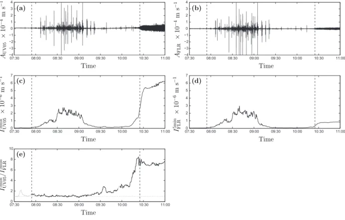
phases (figure 2 a and b). During the first phase, which lasted for about an hour, a high 57
level of seismicity was recorded followed by a relatively quiet phase that directly precede 58
the onset of the eruption (seismic tremor). 59
As a first stage of data processing we correct the signal from the sensor and acquisition 60
sensitivity to retrieve accurate values of ground motion velocity. Seismic signal amplitudes 61
have also been corrected from site effects using the coda amplification factor method 62
[Battaglia and Aki, 2003]. 63
Seismicity induced by magma migration presents a relatively high frequency content 64
compared to the permanent back-ground noise. For this study we will only consider a 65
frequency range between 5Hz and 15Hz. 66
We calculate the envelope of the signal, E, using the norm between the filtered data, 67
x, and their Hilbert transform, H: 68
To eliminate spikes or glitches we decimate the data by keeping the median of 1000 con-69
secutive points, corresponding to 10 seconds. This leads to the seismic intensity estimate, 70
I, that we will use from now. 71
The last step of the analysis is a median filter applied on I using a sliding window of 72
given duration ∆t. 73
The nomenclature used is :
ISta ,∆t (7)
with Sta corresponding to the name of the station. Figure 2 c and d represents the results 74
of this data processing for ∆t = 5min. 75
To highlight relative changes of intensity between different stations we plot the ratio 76
I∆t
Sta1/I
∆t
Sta2 (one example is shown figure 2 e).
77
4. Results
Ratios for different pairs of stations are shown figure 3 a. It is important to note that 78
since this method relies on the seismo-acoustic emmissions from the dike’s tip, we only 79
show results corresponding to periods when signal intensities I∆t
Sta are at least twice the
80
background seismic noise intensity level. 81
We also compare observations of intensity ratios to synthetic itensity ratios at station 82
UV05 and FLR (figure 3 b and c) using a theoretical vertical pathway beneath the eruptive 83
vent and a constant propagation velocity from sea level (0 meters a.s.l at 07:54 AM) to 84
the surface (2500 m at 10:25 AM). The intensity ratios are calculated using equation 3 85
for different value for the quality factor (Q) and both volumetric and surface attenuation 86
(respectively n = 1 and n = 0.5). An interesting point is the behaviour of the theoretical 87
curve that presents an apparent acceleration since the migration is set to be at constant 88
speed. 89
Interestingly the beginning of the seismic swarm (07:54 to 09:00 AM) shows a high level 90
of seismicity with intensity ratios close to unity and with no significant variations which 91
can be interpreted as a slow migration of the magma. In the later part of the seismic 92
swarm (09:00 AM to 10:25 AM) seismic activity strongly decreases and intensity ratios 93
show strong variations. This can be interpreted as a fast migration of the magma in the 94
shallow part of the edifice. This migration presents some heterogeneity with a phase of 95
arrest around 10:00 AM. 96
Simple modelling does not explain the temporal change of the intensity ratio and shows 97
that simple migration is not likely to occur in natural systems. Nevertheless, the intensity 98
ratio during the tremor can be explained using n = 1 and Q ∼ 200, which does not seem 99
a reasonable value for the quality factor, or using n = 0.5 and Q ∼ 50, which implies 100
that the computed seismic intensities are dominated by surface waves. This Q value is in 101
agreement with previous studies [Battaglia and Aki, 2003; Battaglia et al., 2005]. 102
Regarding the ratio presented figure 3 a, the change at 10:09 AM could be due to 103
a change in the direction of the propagation from vertical to horizontal toward station 104
UV05. This highlights the need to develop an inverse problem to extract the position of 105
the propagating front from all the possible intensity ratios. 106
5. Inverse problem
In order to image magma propagation at depth, we seek the best position within a grid 107
that best explains the intensity ratios from all possible pairs of stations. We process a 108
simple inverse problem in which we compute all the theoretical intensity ratios on each 109
point of the grid defined as follows: Easting from 362 km to 370 km every 100m, Northing 110
from 7647 km to 7653 km every 100 m and depth from -0.5 km to 2.5 km above see level 111
every 50 m. The limitation in depth comes from the localisation of individual events at 112
the beginning of the seismic swarm. Parameters used for the attenuation law are n = 0.5 113
and Q = 50. 114
The 3-dimensional misfit used is the following : 115 χ = v u u u u u t X i X j>i I∆t Stai I∆t Staj calculated − I∆t Stai I∆t Staj measured 2 . (8)
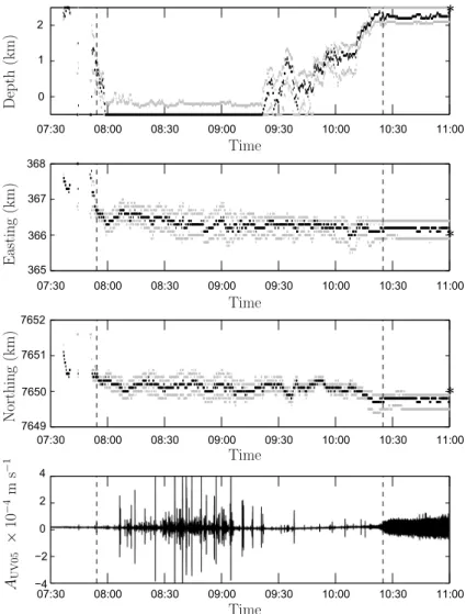
The results are shown figure 4. During the period of high seismic activity, locations 116
are saturated at see level which is consistent with commonly observed seismicity on PdF 117
volcano and the location of single events at the beginning of seismic swarms. As already 118
observed in figure 3, the inversion results show a phase of arrest around 10:00 AM. 119
6. Discussions and Conclusions
The proposed analysis will find a limitation when the source of the seismicity is far 120
from all the stations. In that case, the relative difference in the source-receiver paths are 121
negligible and all the possible intensity ratios will be close to one. This also implies, for 122
future inversion of the migration using intensity ratios, that the error on the position will 123
be a function of the position itself: the greater the source-receiver distance, the greater 124
the error will be. 125
In term of the dynamics of magma propagation, the results clearly show that the upward 126
migration started between 9:00 AM and 9:30 AM. Combining intensity ratios (figure 3) 127
and the results of the inversion (figure 4) we can infer that the migration initiates at 9:00 128
AM with clear migration toward the surface at 9:25 AM which corresponds to about one 129
hour after the beginning of the seimic swarm. At smaller scale the upward propagation 130
does not occur at constant velocity but presents phases of rapid propagation and phases 131
of arrest or with a strong decrease of velocity. 132
This simple analysis can be easily applied to the real time monitoring of magma migra-133
tion and gives an opportunity to extract information on the dynamics of magma propa-134
gation. 135
Acknowledgments. The data used for the analysis were collected by the Institut 136
de Physique du Globe de Paris, Observatoire Volcanologique du Piton de la Fournaise 137
(IPGP/OVPF) and the Laboratoire de G`eophysique Interne et Tectonophysique (LGIT) 138
within the framework of ANR 08 RISK 011/UnderVolc project. The sensors are prop-139
erties of the r´eseau sismologique mobile Fran¸cais, Sismob (INSU-CNRS). We are grate-140
ful to Daniel Clarke for fruitful comments about the manuscript. This work has been 141
supported by ANR (France) under contracts 05-CATT-010-01 (PRECORSIS), ANR-06-142
CEXC-005 (COHERSIS), ANR-08-RISK-011 (UNDERVOLC) and by a FP7 European 143
Research Council advanced grant 227507 (WHISPER). This is IPGP contribution num-144
ber XXXX. 145
References
Aoki, Y., P. Segall, T. Kato, P. Cervelli, and S. Shimada, Imaging magma transport 146
during the 1997 seismic swarm off the Izu Peninsula, Japan, Science, 286, 927–930, 147
1999. 148
Battaglia, J., and K. Aki, Location of seismic events and eruptive fissures on the Piton 149
de la Fournaise volcano using seismic amplitudes, J. Geophys. Res., 108, 2364, doi: 150
10.1029/2002JB002193, 2003. 151
Battaglia, J., K. Aki, and V. Ferrazzini, Location of tremor sources and estimation of lava 152
output using tremor source amplitude on the Piton de la Fournaise volcano: 1. Location 153
of tremor sources, Journal of Volcanology and Geothermal Research, 147, 268–290, doi: 154
10.1016/j.jvolgeores.2005.04.005, 2005. 155
Battaglia, J., V. Ferrazzini, T. Staudacher, K. Aki, and J.-L. Chemin´ee, Pre-eruptive 156
migration of earthquakes at the Piton de la Fournaise volcano (R´eunion Island), Geo-157
phys. J. Int., 161, 549–558, 2005. 158
Hayashi, Y., and Y. Morita, An image of magma intrusion process inferred from pre-159
cise hypocentral migration of the earthquake swarm east of the Izu Peninsula, Geo-160
phys. J. Int., 153, 159–174, 2003. 161
Rubin, A. M., and D. Gillard, Dike-induced earthquakes: Theoretical considerations, 162
J. Geophys. Res., 103, 10,017–10,030, 1998. 163
7644 7646 7648 7650 7652 7654 7656 Northing (km) 362 364 366 368 370 372 374 376 378 Easting (km) 21°S 55°30'E UV11 UV12 FLR UV05 FJS 10 km SNE RVL FOR
Figure 1. Location of Piton de la Fournaise volcano on La R´eunion island (inset) and seismic station distribution (inverted triangles). Those used in this study are referred by their names on the map. The position of the January 2010 eruptive fissure is shown as a dashed circle.
07:30 08:00 08:30 09:00 09:30 10:00 10:30 11:00 −4 −3 −2 −1 0 1 2 3 4 07:30 08:00 08:30 09:00 09:30 10:00 10:30 11:00 0 1 2 3 4 5 6 7 07:30 08:00 08:30 09:00 09:30 10:00 10:30 11:00 −4 −3 −2 −1 0 1 2 3 4 07:30 08:00 08:30 09:00 09:30 10:00 10:30 11:00 0 1 2 3 4 5 6 7 07:30 08:00 08:30 09:00 09:30 10:00 10:30 11:00 0 2 4 6 8 10 (a) (b) (c) (d) (e) Time Time Time Time Time AU V 0 5 × 10 − 4m s − 1 AF L R × 10 − 4m s − 1 I 5 m in U V 0 5 × 10 − 6m s − 1 I 5 m in F L R × 10 − 6m s − 1 I 5 m in U V 0 5 /I 5 m in F L R
Figure 2. Example of data processing. a and b represent the raw ground velocity
at stations UV05 and FLR respectively. c and d represent the seismic intensities, see section 3 for further details. e represents the ratio between I5minUV05 and IFLR . Vertical5min dashed lines represent the beginning of the seismic swarm (07:54 AM) and the onset of the eruption (10:25 AM).
07:30 08:00 08:30 09:00 09:30 10:00 10:30 11:00 0 2 4 6 8 10 07:30 08:00 08:30 09:00 09:30 10:00 10:30 11:00 −4 −2 0 2 4 07:30 08:00 08:30 09:00 09:30 10:00 10:30 11:00 0 2 4 6 8 10 07:30 08:00 08:30 09:00 09:30 10:00 10:30 11:00 0 2 4 6 8 10 (a) (b) (c) (d) I5min UV05/I 5min FLR I5min UV11/I 5min FLR I5min UV11/I 5min UV12 I5min UV05/I 5min FJS I5min UV11/I 5min FJS n = 1 Q = 25 Q = 50 Q = 100 Q = 200 n = 0.5 Q = 25 Q = 50 Q = 100 Q = 200 Time Time Time Time I5min Sta1 I5min Sta2 I5min UV05 I5min FLR I5min UV05 I5min FLR AU V 05 × 10 − 4m s − 1
Figure 3. a, Seismic intensity ratio for five different station pairs (∆t = 5min).
Comparison of real and synthetic ratios for station pair UV05, FLR using different quality factors and considering body wave (b) or surface wave (c) attenuation (respectively, n = 1 and n = 0.5). The synthetic curves are calculated for a source migrating at constant vertical velocity from sea level at 07:54 AM to the vent at 10:25 AM. d represents the raw seismic signal at station UV05 for timing comparison. Vertical dashed lines represent the beginning of the seismic swarm (07:54 AM) and the onset of the eruption (10:25 AM).
07:30 08:00 08:30 09:00 09:30 10:00 10:30 11:00 07:30 08:00 08:30 09:00 09:30 10:00 10:30 11:00 −4 −2 0 2 4 07:30 08:00 08:30 09:00 09:30 10:00 10:30 11:00 07:30 08:00 08:30 09:00 09:30 10:00 10:30 11:00 7651 7652 7650 7649 367 368 366 365 1 2 0 * * * Time Time Time Time D ep th (k m ) E as ti n g (k m ) N or th in g (k m ) AU V 05 × 10 − 4m s − 1
Figure 4. Inversion results. The top three panels show the results of the inversion in terms of depth (above sea level), Easting and Northing. For each component, the black curve represents the best position of the minimum misfit and both grey curve represent the minimum and maximum extension of a volume including misfit values inferior to 10% of the minimum misfit. The bottom panel represents the seismic signal at station UV05 for timing comparison. Vertical dashed lines represent the beginning of the seismic swarm (07:54 AM) and the onset of the eruption (10:25 AM). The black stars show the location of the eruptive fissure.