Validation of ACE-FTS N₂O measurements

HAL Id: hal-00328310

https://hal.archives-ouvertes.fr/hal-00328310

HAL is a multi-disciplinary open access

archive for the deposit and dissemination of sci-entific research documents, whether they are pub-lished or not. The documents may come from teaching and research institutions in France or abroad, or from public or private research centers.

L’archive ouverte pluridisciplinaire HAL, est destinée au dépôt et à la diffusion de documents scientifiques de niveau recherche, publiés ou non, émanant des établissements d’enseignement et de recherche français ou étrangers, des laboratoires publics ou privés.

Validation of ACE-FTS N2O measurements

K. Strong, M. A. Wolff, T. E. Kerzenmacher, K. A. Walker, P. F. Bernath, T.

Blumenstock, C. Boone, Valéry Catoire, M. Coffey, M. de Mazière, et al.

To cite this version:

K. Strong, M. A. Wolff, T. E. Kerzenmacher, K. A. Walker, P. F. Bernath, et al.. Validation of ACE-FTS N2O measurements. Atmospheric Chemistry and Physics Discussions, European Geosciences Union, 2008, 8 (1), pp.3597-3663. �hal-00328310�

ACPD

Full Screen / Esc

Printer-friendly Version Interactive Discussion

EGU

Atmos. Chem. Phys. Discuss., 8, 3597–3663, 2008 www.atmos-chem-phys-discuss.net/8/3597/2008/ © Author(s) 2008. This work is licensed

under a Creative Commons License.

Atmospheric Chemistry and Physics Discussions

Validation of ACE-FTS N

₂

O measurements

K. Strong1, M. A. Wolff1, T. E. Kerzenmacher1, K. A. Walker1,2, P. F. Bernath2,3, T. Blumenstock4, C. Boone2, V. Catoire5, M. Coffey6, M. De Mazi `ere7,

P. Demoulin8, P. Duchatelet8, E. Dupuy2, J. Hannigan6, M. H ¨opfner4, N. Glatthor4, D. W. T. Griffith9, J. J. Jin10, N. Jones9, K. Jucks11, H. Kuellmann12,

J. Kuttippurath12,13, A. Lambert14, E. Mahieu8, J. C. McConnell10, J. Mellqvist15, S. Mikuteit4, D. P. Murtagh15, J. Notholt12, C. Piccolo16, P. Raspollini17,

M. Ridolfii18, C. Robert5, M. Schneider4, O. Schrems19, K. Semeniuk10,

C. Senten7, G. P. Stiller4, A. Strandberg15, J. Taylor1, C. T ´etard20, M. Toohey1, J. Urban15, T. Warneke12, and S. Wood21

1

Department of Physics, University of Toronto, Toronto, Ontario, Canada

2

Department of Chemistry, University of Waterloo, Waterloo, Ontario, Canada

3

Department of Chemistry, University of York, York, UK

4

Forschungszentrum Karlsruhe and University of Karlsruhe, Institute for Meteorology and Climate Research (IMK), Karlsruhe, Germany

5

Laboratoire de Physique et Chimie de L’Environment CNRS - Universit ´e d’Orl ´eans, Orl ´eans, France

6

National Center for Atmospheric Research, Boulder, Colorado, USA

7

Belgian Institute for Space Aeronomy, Brussels, Belgium

8

ACPD

Full Screen / Esc

Printer-friendly Version Interactive Discussion

EGU 9

School of Chemistry, University of Wollongong, Wollongong, Australia

10

Department of Earth and Space Science and Engineering, York University, Toronto, Ontario, Canada

11

Harvard-Smithsonian Center for Astrophysics, Cambridge, Massachusetts, USA

12

Institute for Environmental Physics, University of Bremen, Bremen, Germany

13

now at: LMD/CNRS Ecole Polytechnique, Palaiseau Cedex, France

14

Jet Propulsion Laboratory, California Institute of Technology, Pasadena, California, USA

15

Department of Radio and Space Science, Chalmers University of Technology, Gothenburg, Sweden

16

Department of Physics, University of Oxford, Oxford, UK

17

Institute of Applied Physics “Nello Carrara”, National Research Center, Firenze, Italy

18

Dipartimento di Chimica Fisica e Inorganica, Universit `a di Bologna, Bologna, Italy

19

Alfred Wegener Institute for Polar and Marine Research, Bremerhaven, Germany

20

Laboratoire d’Optique Atmosph ´erique, Universit ´e des sciences et technologies de Lille, Villeneuve d’Ascq, France

21

National Institute of Water and Atmospheric Research Ltd., Lauder, New Zealand

Received: 28 November 2007 – Accepted: 18 January 2008 – Published: 21 February 2008 Correspondence to: K. Strong ([email protected])

ACPD

Full Screen / Esc

Printer-friendly Version Interactive Discussion

EGU

Abstract

The Atmospheric Chemistry Experiment (ACE), also known as SCISAT, was launched on 12 August 2003, carrying two instruments that measure vertical profiles of atmo-spheric constituents using the solar occultation technique. One of these instruments, the ACE Fourier Transform Spectrometer (ACE-FTS), is measuring volume mixing ratio

5

(VMR) profiles of nitrous oxide (N₂O) from the upper troposphere to the lower meso-sphere at a vertical resolution of about 3–4 km. In this study, the quality of the ACE-FTS version 2.2 N₂O data is assessed through comparisons with coincident measurements made by other satellite, balloon-borne, aircraft, and ground-based instruments. These consist of vertical profile comparisons with the SMR, MLS, and MIPAS satellite

in-10

struments, multiple aircraft flights of ASUR, and single balloon flights of SPIRALE and FIRS-2, and partial column comparisons with a network of ground-based Fourier Trans-form InfraRed spectrometers (FTIRs). Overall, the quality of the ACE-FTS version 2.2 N₂O VMR profiles is good over the entire altitude range from 5 to 60 km. Between 6 and 30 km, the mean absolute differences for the satellite comparisons lie between

15

−42 ppbv and +17 ppbv, with most within ±20 ppbv. This corresponds to relative devi-ations from the mean that are within ±15%, except for comparisons with MIPAS near 30 km, for which they are as large as 22.5%. Between 18 and 30 km, the mean abso-lute differences are generally within ±10 ppbv, again excluding the aircraft and balloon comparisons. From 30 to 60 km, the mean absolute differences are within ±4 ppbv,

20

and are mostly between −2 and +1 ppbv. Given the small N2O VMR in this region,

the relative deviations from the mean are therefore large at these altitudes, with most suggesting a negative bias in the ACE-FTS data between 30 and 50 km. In the compar-isons with the FTIRs, the mean relative differences between the ACE-FTS and FTIR partial columns are within ±6.6% for eleven of the twelve contributing stations. This

25

mean relative difference is negative at ten stations, suggesting a small negative bias in the ACE-FTS partial columns over the altitude regions compared. Excellent correlation (R=0.964) is observed between the ACE-FTS and FTIR partial columns, with a slope

ACPD

Full Screen / Esc

Printer-friendly Version Interactive Discussion

EGU

of 1.01 and an intercept of −0.20 on the line fitted to the data.

1 Introduction

Nitrous oxide (N₂O) is an important atmospheric constituent, as it is the primary source gas for nitrogen oxides in the stratosphere, a useful dynamical tracer, and an effi-cient greenhouse gas. N₂O has many surface and near-surface sources, with

ap-5

proximately equal contributions from natural and anthropogenic emissions. Natural sources include biological nitrogen cycling in the oceans and soils and oxidation of NH₃, while anthropogenic sources include chemical conversion of nitrogen in fertilizers into N₂O, biomass burning, cattle, and some industrial activities (IPCC, 2007). It is the only long-lived atmospheric tracer of human perturbations of the global nitrogen

10

cycle (Holland et al.,2005). There are large uncertainties in N₂O source strengths de-rived from emissions inventories, with estimates of the total source strength varying by ±50% (McLinden et al.,2003, and references therein). Tropospheric N₂O is trans-ported through the tropical tropopause into the stratosphere, where approximately 90% is destroyed by photolysis at wavelengths from 185 to 220 nm, which creates N₂ and

15

O. The remaining 10% is destroyed by reaction with O1D. The latter has two channels, one of which generates two NO molecules and serves as the source for stratospheric nitrogen oxides, which participate in catalytic destruction of ozone (Bates and Hays,

1967;Crutzen,1970;McElroy and McConnell,1971).

While N₂O is well-mixed in the troposphere, its concentration decays with altitude in

20

the stratosphere due to the reactions noted above. Its photochemical lifetime varies from approximately 100 years at 20 km and below, to 1 year at 33 km and 1 month at 40 km (Brasseur and Solomon, 2005). As these lifetimes are longer than dynamical time scales, the global distribution of N₂O is primarily governed by the Brewer-Dobson circulation. This makes it a useful tracer in the stratosphere, both as a diagnostic tool in

25

atmospheric models (Mahlman et al.,1986;Holton,1986;Bregman et al.,2000;Plumb

ACPD

Full Screen / Esc

Printer-friendly Version Interactive Discussion

EGU

interpretation of observational data. For example, N₂O has been used in numerous studies of polar vortex dynamics and chemistry (e.g.,Proffitt et al.,1989,1990,1992;

M ¨uller,1996;Bremer et al.,2002; Urban et al.,2004), the tropical pipe (e.g., Plumb,

1996;Murphy et al.,1993;Volk et al.,1996;Minschwaner et al.,1996; Avallone and

Prather, 1996), transport and chemistry in the upper troposphere/lower stratosphere

5

(e.g.,Boering et al.,1994;Hegglin et al.,2006), and global transport processes (e.g.,

Randel et al.,1993,1994).

Radiatively, N₂O is a long-lived greenhouse gas (Yung et al., 1976; Ramanathan

et al., 1985). It has a global warming potential of 289 over 20 years, and a global average radiative forcing due to increases in N₂O since the pre-industrial era of

10

0.16±0.02 Wm−2_{, making it the fourth most important trace gas contributing to}

posi-tive forcing (IPCC,2007). Global surface concentrations of atmospheric N₂O are cur-rently increasing at about 0.26% per year, and have risen from a pre-industrial value of about 270 ppbv to 319 ppbv in 2005, due to an increase of 40–50% in surface emis-sions over that period due to human activities (Battle et al., 1996; Fl ¨uckiger et al.,

15

1999; Zander et al., 2005; Hirsch et al., 2006; WMO, 2006; IPCC, 2007, and

refer-ences therein). There is a hemispheric difference in N2O, with about 0.8 ppbv more in

the northern hemisphere, which is the source of approximately 60% of the emissions

(Brasseur and Solomon,2005).

Global distributions of N₂O have been measured from space since 1979, when

20

the Stratospheric and Mesospheric Sounder (SAMS) on Nimbus 7 began operations

(Drummond et al.,1980; Jones and Pyle,1984; Jones et al.,1986). SAMS used an

infrared pressure modulator radiometer to measure thermal emission from the limb at 7.8µm, from which stratospheric N₂O profiles were retrieved until 1983. This was fol-lowed by the Improved Stratospheric and Mesospheric Sounder (ISAMS) and the

Cryo-25

genic Limb Array Etalon Spectrometer (CLAES) on the Upper Atmosphere Research Satellite (UARS). ISAMS also used pressure modulator radiometers, operating from 4.6 to 16.3µm, and provided N₂O profiles between October 1991 and July 1992 (

ACPD

Full Screen / Esc

Printer-friendly Version Interactive Discussion

EGU

using thermal limb emission, from 3.5 to 13µm, between October 1991 and May 1993

(Roche et al.,1993,1996). The Atmospheric Trace Molecule Spectroscopy (ATMOS)

instrument, flown on four Space Shuttle missions, first on Spacelab-3 in 1985 and sub-sequently on Atmospheric Laboratory for Applications and Science (ATLAS)-1, -2, and -3 in 1992, 1993, and 1994, made the first infrared solar occultation measurements of

5

N₂O from space (Abrams et al.,1996;Gunson et al.,1996;Michelsen et al.,1998;Irion

et al.,2002). Also flown on ATLAS-3, in 1994, was the CRyogenic Infrared Spectrom-eters and Telescopes for the Atmosphere (CRISTA), which used four spectromSpectrom-eters to measure emission in the limb at mid-infrared (4–14µm) and far-infrared (15–71 µm)

wavelengths (Offermann et al., 1999;Riese et al.,1999). The Improved Limb

Atmo-10

spheric Spectrometer (ILAS) and ILAS-II instruments on the Advanced Earth Observ-ing Satellite (ADEOS) and ADEOS-II, respectively, both measured N₂O using infrared solar occultation. ILAS made measurements from September 1996 to June 1997 (

Kan-zawa et al., 2003; Khosrawi et al., 2004), while ILAS-II operated for eight months in 2003 (Ejiri et al.,2006;Khosrawi et al.,2006).

15

There are currently four satellite instruments in orbit measuring N₂O. One of these is the Atmospheric Chemistry Experiment Fourier Transform Spectrometer (ACE-FTS) on SCISAT, launched in 2003 (Bernath et al., 2005). The others are the Sub-Millimetre Ra-diometer (SMR) on Odin, launched in 2001 (Murtagh et al.,2002;Urban et al.,2005a,b,

2006), the Michelson Interferometer for Passive Atmospheric Sounding (MIPAS) on

En-20

visat, launched in 2002 (Fischer et al.,2007), and the Microwave Limb Sounder (MLS) on the Aura satellite (Waters et al., 2006; Lambert et al., 2007), launched in 2004. These are described in more detail below.

The objective of this study is to assess the quality of the ACE-FTS version 2.2 N₂O data, prior to its public release, through comparisons with coincident measurements.

25

The paper is organized as follows. In Sect. 2, the ACE mission and the N₂O re-trievals are briefly described. Section 3 outlines the methodology used to compare and present the validation results. In Sect. 4, the results of vertical profile comparisons with the SMR, MLS, and MIPAS satellite instruments are discussed. Section 5

fo-ACPD

Full Screen / Esc

Printer-friendly Version Interactive Discussion

EGU

cuses on the results of comparisons with data from the ASUR (Airborne SUbmillimeter wave Radiometer) aircraft flights and from the SPIRALE (SPectroscopie Infra-Rouge d’Absorption par Lasers Embarqu ´es) and FIRS-2 (Far-InfraRed Spectrometer-2) bal-loon flights. Partial column comparisons with a network of ground-based Fourier Trans-form InfraRed spectrometers (FTIRs) are presented in Sect. 6. Finally, the results are

5

summarized and conclusions regarding the quality of the ACE-FTS version 2.2 N₂O data are given in Sect. 7.

2 ACE-FTS N₂O retrievals

The Atmospheric Chemistry Experiment has been in orbit since its launch on 12 Au-gust 2003. ACE is a Canadian-led satellite mission, also known as SCISAT, which

10

carries two instruments, the ACE-FTS (Bernath et al., 2005) and the Measurement of Aerosol Extinction in the Stratosphere and Troposphere Retrieved by Occultation (ACE-MAESTRO) (McElroy et al., 2007). Both instruments record solar occultation spectra, ACE-FTS in the infrared (IR), and MAESTRO in the ultraviolet-visible-near-IR, from which vertical profiles of atmospheric trace gases, temperature, and aerosol

ex-15

tinction are retrieved. The SCISAT spacecraft is in a circular orbit at 650-km altitude, with a 74◦ _{inclination angle (Bernath et al.,2005), providing up to 15 sunrise and 15}

sunset solar occultations per day. The choice of orbital parameters results in coverage of the tropics, mid-latitudes and polar regions with an annually repeating pattern, and a sampling frequency that is greatest over the Arctic and Antarctic. The primary

scien-20

tific objectives of the ACE mission are: (1) to understand the chemical and dynamical processes that control the distribution of ozone in the stratosphere and upper tropo-sphere, particularly in the Arctic; (2) to explore the relationship between atmospheric chemistry and climate change; (3) to study the effects of biomass burning on the free troposphere; and (4) to measure aerosols and clouds to reduce the uncertainties in

25

their effects on the global energy balance (Bernath et al.,2005;Bernath, 2006, and references therein).

ACPD

Full Screen / Esc

Printer-friendly Version Interactive Discussion

EGU

ACE-FTS measures atmospheric spectra between 750 and 4400 cm−1_{(2.2–13µm)}

at 0.02 cm−1resolution (Bernath et al., 2005). Profiles as a function of altitude for pres-sure, temperature, and over 30 trace gases are retrieved from these spectra. The de-tails of ACE-FTS processing are described inBoone et al.(2005). Briefly, a non-linear least squares global fitting technique is employed to analyze selected microwindows

5

(0.3–30 cm−1 _{wide portions of the spectrum containing spectral features for the}

tar-get molecule). Prior to performing volume mixing ratio (VMR) retrievals, pressure and temperature as a function of altitude are determined through the analysis of CO₂lines in the spectra. Forward model calculations employ the spectroscopic constants and cross-section measurements from the HITRAN 2004 line list (Rothman et al.,2005).

10

First-guess profiles are based on ATMOS measurements, but the retrievals are not sensitive to this a priori information.

The ACE-FTS instrument collects measurements every 2 s, which yields a typical al-titude sampling of 3–4 km within an occultation, neglecting the effects of refraction that compress the spacing at low altitudes. The altitude coverage of the measurements

ex-15

tends from the upper troposphere to as high as 150 km, depending on the constituent. Note that the altitude spacing can range from 1.5 to 6 km, depending on the geometry of the satellite’s orbit for a given occultation. The actual altitude resolution achievable with the ACE-FTS is limited to about 3–4 km, a consequence of the instrument’s field-of-view (1.25-mrad-diameter aperture and 650-km altitude). Atmospheric quantities

20

are retrieved at the measurement heights. For the purpose of generating calculated spectra (i.e., performing forward model calculations), quantities are interpolated from the measurement grid onto a standard 1-km grid using piecewise quadratic interpola-tion. The comparisons in this work use the ACE-FTS VMR profiles on the 1-km grid.

N₂O is one of the 14 primary target species for the ACE mission. A total of

25

69 microwindows are used in the version 2.2 ACE-FTS retrievals for N₂O. They are in the wavenumber ranges 1120–1280, 1860–1951, 2180–2240, 2440–2470, and 2510– 2600 cm−1_{. The altitude range for the retrieval extends from 5 to 60 km. The primary}

ACPD

Full Screen / Esc

Printer-friendly Version Interactive Discussion

EGU

species are retrieved simultaneously with N₂O. The precision of the ACE-FTS N₂O VMRs is defined as the 1σ statistical fitting errors from the least-squares process,

as-suming a normal distribution of random errors (Boone et al.,2005). We have examined these fitting errors for the ACE-FTS N₂O profiles used in the comparisons with MLS (Sect. 4.2), and found that the median value is<3% from 5–45 km, increasing to 17%

5

at 60 km, while the mean value is<4% from 5–35 km, and oscillating above this due to

some outliers in the individual percent fitting errors.

To date, ACE-FTS N₂O profiles have been compared with MLS data (Froidevaux

et al., 2006; Lambert et al., 2007; Toohey and Strong, 2007), and partial columns have been compared with those retrieved using the Portable Atmospheric Research

10

Interferometric Spectrometer for the Infrared (PARIS-IR), a ground-based adapta-tion of ACE-FTS, during the spring 2004 Canadian Arctic ACE validaadapta-tion campaign (Sung et al.,2007).

3 Validation approach

The comparisons shown in this work include ACE-FTS data from 21 February 2004

15

(the start of the ACE Science Operations phase) through to 26 February 2007. The coincidence criteria for each correlative dataset were determined in consultation with the teams involved, striving for consistency insofar as possible. The location for each ACE occultation is defined as the latitude, longitude and time of the 30-km tangent point (calculated geometrically), and it is this value that was used in searching for

co-20

incidences. Because N₂O is a long-lived and well-mixed constituent, it was possible to use relatively relaxed temporal and spatial coincidence criteria, thereby providing good statistics for the comparisons. For the global satellite datasets, available for SMR and MLS, the coincidence criteria were defined as ±12 h, ±1◦_{latitude and ±8}◦_{longitude, as}

used byLambert et al.(2007) in the validation of MLS N₂O measurements. Correlative

25

data for MIPAS were only available for a two-month period in early 2004 for northern mid- and high latitudes, and for these, slightly tighter criteria were defined. For the

ACPD

Full Screen / Esc

Printer-friendly Version Interactive Discussion

EGU

ASUR aircraft measurements, obtained during several flights, the coincidence criteria were defined as ±12 h and 1000 km. For the statistical comparisons, unless otherwise noted, multiple counting of profiles was allowed, so that ifn validation measurements

met the criteria with respect to a single ACE-FTS occultation, then these would be in-cluded asn coincidences and the ACE-FTS measurement would be counted n times.

5

Balloon-based single profile measurements by SPIRALE and FIRS-2 obtained within ±26 h and 500 km of ACE occultations were included in the comparisons. Finally, for the ground-based FTIRs, the criteria were set at ±24 h and 1000 km for all but two stations (see Sect. 6), to provide a meaningful number of coincidences. Table1 summarizes the correlative datasets, comparison periods, temporal and spatial coincidence

crite-10

ria, and number of coincidences for the statistical and individual profile comparisons. Information about the FTIR stations and comparisons is provided in Tables2and3 in Sect. 6.

The SMR, MLS, MIPAS, and FIRS-2 VMR profiles all have vertical resolutions that are similar to that of ACE-FTS, and so no smoothing was applied to these data. These

15

correlative profiles were linearly interpolated onto the 1-km ACE altitude grid. MLS profiles, reported on pressure levels, were mapped onto the 1-km altitude grid of ACE by interpolating in log pressure each MLS profile onto the retrieved pressure profile of the coincident ACE-FTS observation. The aircraft-based ASUR instrument has lower vertical resolution than ACE-FTS, so the ACE-FTS profiles were convolved with the

20

ASUR averaging kernels. The balloon-borne SPIRALE VMR profile was obtained at significantly higher vertical resolution than ACE-FTS, and so was convolved with trian-gular functions having full width at the base equal to 3 km and centered at the tangent height of each occultation (see Eq. (1) ofDupuy et al.(2008)). This approach simulates the smoothing effect of the ACE-FTS field-of-view, as discussed byDupuy et al.(2008).

25

The resulting smoothed profiles were then interpolated onto the 1-km grid. Finally, for the comparisons with the ground-based FTIR measurements, which have significantly lower vertical resolution, the ACE-FTS profiles were smoothed by the appropriate FTIR averaging kernels to account for the different vertical sensitivities of the two

measure-ACPD

Full Screen / Esc

Printer-friendly Version Interactive Discussion

EGU

ment techniques. The method ofRodgers and Connor(2003) was followed and Eq. (4) from their paper was applied, using the a priori profile and the averaging kernel matrix of the FTIR. Partial columns over specified altitude ranges were then calculated for both ACE-FTS and the FTIRs, as described in Sect. 6, and these were used in the comparisons.

5

Co-located pairs of vertical VMR profiles from ACE-FTS and each validation experi-ment (referred to as VAL in text and figures below) were identified using the appropriate temporal and spatial coincidence criteria. Then the following procedure was applied to the vertical profile measurements used in this assessment, with some modifications for the individual profile comparisons (SPIRALE and FIRS-2) and the FTIR partial column

10

comparisons (see Sect. 5 and Sect. 6 for details).

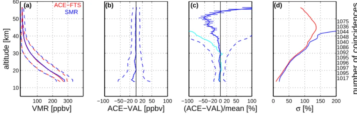
(a) Calculate the mean profile of the ensemble for ACE-FTS and the mean profile for VAL, along with the standard deviations on each of these two profiles. These mean profiles are plotted as solid lines, with ±1σ as dashed lines, in panel (a) of the

com-parison figures discussed below. The standard error on the mean, also known as the

15

uncertainty in the mean, is calculated as σ(z)/pN(z), where N(z) is the number of points used to calculate the mean at a particular altitudez, and is included as error

bars on the lines in panel (a). Note: in some cases, these error bars, as well as those in panels (b) and (c) (see below) may be small and difficult to distinguish.

(b) Calculate the profile of the mean absolute difference, ACE-FTS − VAL, and the

20

standard deviation of the distribution of this mean difference. (Note that the term “ab-solute”, as used in this work, refers to differences between the compared values and not to absolute values in the mathematical sense.) To do this, the differences are first calculated for each pair of profiles at each altitude, and then averaged to obtain the mean absolute difference at altitude z:

25 ∆abs(z) = 1 N(z) N(z) X i =1 [ACE_i(_{z) − VALi}(z)] (1)

ACPD

Full Screen / Esc

Printer-friendly Version Interactive Discussion

EGU

for the ith coincident pair, and VAL_i(z) is the corresponding VMR for the validation

instrument. This mean absolute difference is plotted as a solid line in panel (b) of the comparison figures below, with ±1σ as dashed lines. Error bars are also included in

these figures. For the statistical comparisons involving multiple coincident pairs (SMR, MLS, MIPAS, ASUR), these error bars again represent the uncertainty in the mean.

5

For individual profile comparisons (SPIRALE, FIRS-2), these error bars represent the combined random error, computed as the root-sum-square error of the ACE-FTS fitting error and the error provided for VAL.

(c) Calculate the profile of the mean relative difference, as a percentage, defined using: 10 ∆rel(z) = 100% × 1 N(z) N(z) X i =1 [ACE_i(_{z) − VALi}(z)] [ACE_i(_{z) + VALi}(z)]/2 = 100% × 1 N(z) N(z) X i =1 [ACE_i(_{z) − VALi}(z)] MEAN_i(z) (2)

where MEAN_i(z) is the mean of the two coincident profiles at z for the i th coincident

pair. Panel (c) of the comparison figures presents the mean relative difference as a solid cyan line. In addition, the relative deviation from the mean is calculated for the

15

statistical comparisons using:

∆mean(z) = 100% × 1 N(z) PN(z) i =1 [ACEi(z) − VALi(z)] 1 N(z) PN(z) i =1 [ACEi(z) + VALi(z)]/2 = 100% × 1 N(z) N(z) X i =1 [ACE_i(_{z) − VALi}(z)] MEAN(z)

ACPD

Full Screen / Esc

Printer-friendly Version Interactive Discussion

EGU

= 100% × ∆abs(z)

MEAN(z) (3)

where MEAN(z) is the mean of all pairs of coincident profiles at z, which is equivalent

to the mean of the average ACE-FTS VMR at z and average VAL VMR at z. This

is plotted as the solid dark blue line in panel (c). The relative standard deviation is calculated as the standard deviation on ∆abs(z) from step (b) divided by MEAN(z), and 5

is plotted as dashed lines (±1σ), with the corresponding relative standard error on the mean included as error bars. In the discussions of relative comparisons below, it is ∆mean(z) that is primarily used; this reduces the impact of very small denominators and

noisy data in Eq. (2), which can make ∆rel(z) very large (von Clarmann,2006).

(d) For the statistical comparisons, calculate the relative standard deviations on each

10

of the ACE-FTS and VAL mean profiles calculated in step (a). For individual profile comparisons, the relative values of the ACE-FTS fitting error and the error for VAL are determined instead. These results are plotted in panel (d) of the comparison figures, with selected values of the number of coincident pairs given as a function of altitude on the right-hand y-axis for the statistical comparisons. For clarity, numbers are not given

15

for all levels.

4 Comparisons with satellite measurements

4.1 SMR

The Sub-Millimetre Radiometer (SMR), launched on Odin in February 2001, has four tunable heterodyne radiometers that are used to detect thermal limb

emis-20

sion from atmospheric molecules between 486 and 581 GHz. Odin is in a sun-synchronous, near-terminator orbit at an altitude of ∼600 km and an inclination of 97.8◦

(Murtagh et al.,2002). SMR observes a thermal emission line of N₂O in the limb at

502.3 GHz, and measurements of near-global fields of N₂O are performed on a time-sharing basis with other observation modes on roughly one day out of three, based

ACPD

Full Screen / Esc

Printer-friendly Version Interactive Discussion

EGU

on 14–15 orbits per day and 40–60 limb scans per orbit. Algorithms based on the opti-mal estimation method (Rodgers,2000) are used for SMR profile retrievals. The latest level 2 version is Chalmers v2.1. N₂O profile information is retrieved in the strato-sphere between ∼12 and ∼60 km with an altitude resolution of ∼1.5 km (in the lower stratosphere, degrading above) and a corresponding single profile precision smaller

5

than 30 ppbv (10–15% below 30 km) (Urban et al.,2006). The horizontal resolution is of the order of 300 km, determined by the limb path in the tangent layer. The satellite motion leads to an uncertainty of the mean profile position of similar magnitude. The SMR N_{2O data are validated in the range ∼15–50 km. The systematic error is} esti-mated to be better than 12 ppbv at altitudes above ∼20 km and increases up to values

10

of 35 ppbv (∼10–15%) below (Urban et al.,2005b), consistent with results obtained in the validation studies showing, for example, a good overall agreement within 4–7 ppbv with data from MIPAS (European Space Agency (ESA) operational processor version 4.61) (Urban et al.,2005a,2006).

For this study, only SMR profiles of good quality (assigned Quality flag=0 or 4) were

15

used. The measurement response, provided in the SMR level 2 files for each retrieval altitude, was required to be larger than 0.9 as recommended byUrban et al.(2005a), in order to exclude altitude ranges where a priori information used by the retrieval algorithm for stabilization contributes significantly to the retrieved mixing ratios. The comparisons used coincidence criteria of ±12 h, ±1◦latitude, and ±8◦longitude, and

20

included data from 21 February 2004 to 30 November 2006. This yields 1099 multiple coincident pairs, allowing investigation of the latitudinal behaviour of ACE-FTS–SMR comparisons. In order to exclude extreme outliers, relative differences over 1000% were not included when deriving the mean of the relative differences. This excluded about 2% of the data from the comparison, removing 984 altitudes between 21 and

25

59 km, and leaving 45 690 altitudes for which the relative differences were less than 1000%.

The results of the comparison between ACE-FTS and SMR profiles between 83◦_S

ACPD

Full Screen / Esc

Printer-friendly Version Interactive Discussion

EGU

between the mean N₂O VMR profiles (panel (a)) and in the mean absolute differences (panel (b)) between 15 and 50 km, which is the validated altitude range for SMR N₂O. From 15–50 km, the mean absolute difference is better than −10 ppbv, and is better than −5 ppbv for all but four levels in this altitude range, with ACE-FTS values generally being the smaller of the two, by −2.4 ppbv on average. Comparisons are also shown

5

outside the validated range for SMR (13–15 km and 50–57 km): between 50 and 57 km, the SMR profiles decrease rapidly, leading to larger differences relative to ACE-FTS, varying from −1.5 ppbv at 50.5 km to +1.0 ppbv at 56.5 km.

Figure1c illustrates the difficulty of obtaining useful information from the mean rela-tive difference defined in Eq. (2) for a species such as N₂O, whose VMR decreases to

10

very small values (typically a few ppbv in the upper stratosphere), and for which there are some coincident profiles whose values for each instrument are of the same mag-nitude but opposite sign. In some cases, the denominator in Eq. (2) is zero or close to zero, resulting in very large values. These values strongly affect the mean relative dif-ference, although the number of these cases are relatively small; thus these extremely

15

large values are excluded as stated above. However, the mean relative difference is still affected by the noisiness of SMR data in the upper stratosphere and lower mesosphere, as seen in the relative standard deviation on SMR in Fig.1d. In the upper stratosphere and lower mesosphere where the ACE-FTS N₂O VMR is small and the SMR N₂O VMR is noisy, the denominator in the expression [ACE_i(_z)−VALi(z)]/MEANi(z) is close to

20

half of the SMR VMR and the numerator is close to the SMR VMR, making the ratio approach 200%. As a consequence, the mean relative difference is not a good in-dicator of the agreement between ACE-FTS and SMR at higher altitudes, although it is better than −7% between 15 and 30 km. Figure 1c thus also includes the relative deviation from the mean, as defined in Eq. (3); this shows better agreement between

25

ACE-FTS and SMR, to better than −20%, and to −4% on average, between 15 and 40 km. Between 40 and 50 km, the relative deviation from the mean is as large as −44%, with ACE-FTS consistently smaller. Above 50 km, as the SMR N2O VMRs

ACPD

Full Screen / Esc

Printer-friendly Version Interactive Discussion

EGU

with a maximum value of +127% at 56.5 km. These larger values are consistent with the noisier data, particularly from SMR, above 40 km, as seen in the relative standard deviations on the mean profiles plotted in Fig.1d.

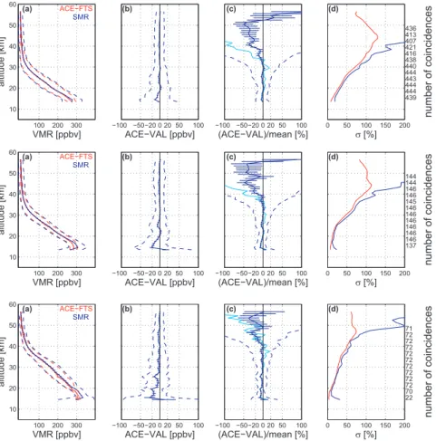
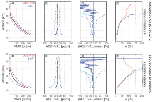
The data shown in Fig. 1 have been subdivided into five latitude bands in Fig. 2: 60–90◦_{N, 30–60}◦_{N, 30}◦_S–30◦_{N, 30–60}◦_{S, and 60–90}◦_{S. The latitudinal gradients in} 5

N₂O are small at the lower and higher altitudes, as can be seen when comparing the mean profiles for each zonal band. However, a clear latitudinal gradient can be seen in the mid-stratosphere; for example, at 30 km, the mean ACE-FTS VMR is 155 ppbv for 30◦_S–30◦_{N, dropping in the mid-latitudes to 82 (63) ppbv for 30–60}◦_{S (N), and}

down to 35 ppbv in the polar regions of both hemispheres. Very similar behaviour is

10

seen in the SMR mean profiles. The mean absolute differences are similar in the five bands, with ACE-FTS being consistently slightly smaller than SMR between 15 and 50 km, with the exception of a few levels in each case. These differences are again typically about −2 ppbv, with maximum values of −7 ppbv from 60–90◦_{N, −18 ppbv}

from 30–60◦_{N, −27 ppbv from 30}◦_S–30◦_{N (at 15.5 km with only 22 coincident pairs),} 15

−11 ppbv from 30–60◦S, and −10 ppbv from 60–90◦S. The mean relative differences remain less than 8% between 15 and 30 km, for all but two levels (−13% at 28.5 km for 60–90◦_{S and −16% at 29.5 km for 60–90}◦_{N). There is more variability between}

the latitude bands in the relative deviations from the mean; these are typically better than 5% between 12 and 40 km, with maxima of −24% from 60–90◦_{N, −29% from 30–} 20

60◦_{N, −8% from 30}◦_S–30◦_{N, −40% from 30–60}◦_{S (at 12.5 km with only 25 coincident}

pairs (not labelled)), and −17% from 60–90◦S. The relative deviations from the mean increase above 40 km, where the relative standard deviations on the mean profiles are also seen to reach values of 100% and larger.

4.2 MLS

25

The Microwave Limb Sounder (MLS) was launched on the Aura satellite in July 2004. It is in a sun-synchronous orbit at an altitude of 705 km and an inclination of 98◦_{, with}

ACPD

Full Screen / Esc

Printer-friendly Version Interactive Discussion

EGU

Global measurements are obtained daily from 82◦_{S to 82}◦_{N, with 240 scans per orbit.}

Like SMR, MLS measures atmospheric thermal emission from the limb, using seven radiometers to provide coverage of five spectral regions between 118 GHz and 2.5 THz. Volume mixing ratio profiles of N₂O are retrieved from the thermal emission line at 652.83 GHz using the optimal estimation approach described byLivesey et al.(2006).

5

The retrieval is performed on a pressure grid with six levels per decade for pressures greater than 0.1 hPa and three levels per decade for pressures less than 0.1 hPa. The vertical resolution for N₂O VMR profiles is 4–6 km, the along-track horizontal resolution is 300–600 km, and the recommended pressure range for the use of individual profiles is 100–1 hPa (Livesey et al.,2007).

10

For the comparisons in this work, MLS version 2.2 is used. Validation of the v2.2 N₂O data product is described byLambert et al.(2007), whileFroidevaux et al.(2006) discuss initial validation of MLS v1.5 data products, including N₂O. The precision of individual v2.2 N_{2O profiles is estimated to be ∼13–25 ppbv (7–38%) for pressures} between 100 and 4.6 hPa, while the accuracy is 3–70 ppbv (9–25%) over the same

15

pressure range (Lambert et al., 2007). Initial comparisons between MLS v2.2 and ACE-FTS v2.2 N₂O indicated agreement in the mean percentage difference profiles to better than ±5% over 100–1 hPa, with MLS showing a low bias (within −5%) for pressures_{>32 hPa and a high bias (within +5%) for lower pressures. Analysis of the} latitudinal behaviour of the mean absolute difference showed that MLS is consistently

20

smaller than ACE-FTS at most latitudes for pressures between 100 and 32 hPa. Dif-ferences were somewhat smaller for ACE-FTS sunrise occultations than for sunset at 46–10 hPa.

Lambert et al.(2007) used an initial subset of the MLS v2.2 reprocessed data, which

provided 1026 coincidences for the comparisons with ACE-FTS N₂O. These were

ob-25

tained over 121 days between September 2004 and October 2006. The present study extends the analyses of Lambert et al. (2007), using data from 16 September 2004 through 26 February 2007, which includes 6876 pairs using coincidence criteria of ±12 h, ±1◦_{latitude, ±8}◦_{longitude, and multiple counting. The MLS data used in this}

ACPD

Full Screen / Esc

Printer-friendly Version Interactive Discussion

EGU

work are screened based on the recommended parameters: even values of the Sta-tus field, Quality values greater than 0.5, Convergence values less than 1.55, positive precision, and pressure levels between 100 and 1 hPa (Livesey et al.,2007;Lambert

et al.,2007). ACE-FTS data were filtered by removing profiles flagged as Do Not Use (DNU) (seehttps://databace.uwaterloo.ca/validation/data issues.php). For the period

5

of MLS coincidences, this removed only one DNU occultation.

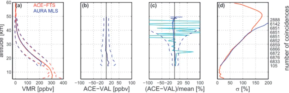
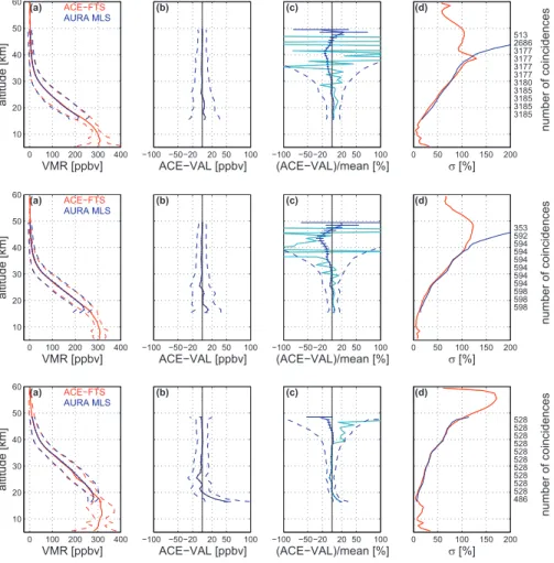
Figure 3shows the results of the comparison between ACE-FTS and MLS profiles from 82◦_{S and 82}◦_{N. Excellent agreement is seen over all altitudes, with the mean}

absolute difference between −3 and +10 ppbv from 15 to 50 km, with differences of 1 ppbv on average over this altitude range, and better than 4 ppbv above 20 km. The

10

mean relative difference exhibits large oscillations, which result from some coincident profiles whose values for each instrument are of the same magnitude but opposite sign, leading to extremely small (or infinitesimal) values of the calculated mean. Di-viding by infinitesimal values in (Eq. 2) leads to very large outlying values, as has been confirmed by an examination of all the individual profiles of ACE_i(_z)−VALi(z)

15

and of [ACE_i(z)−VALi(z)]/MEANi(z), the latter including some significant outliers. His-tograms of the ACE-FTS and MLS N₂O VMRs, their differences, and their relative means were constructed at particular altitudes, and also confirmed this behaviour. In contrast, the relative deviation from the mean (solid blue line in Fig.3c) is well behaved, with ACE-FTS agreeing to within ±7% from 15–50 km. Below 24 km, ACE-FTS has a

20

high bias of +5 ppbv on average (10 ppbv maximum), with the relative deviation from the mean better than +3% on average (+5% maximum). Above 24 km, ACE-FTS has a low bias of −1 ppbv on average (−3 ppbv maximum), with the relative deviation from the mean better than −4% on average (−7% maximum). These results are consistent

with Lambert et al. (2007), with the exception of the slightly larger relative deviation

25

from the mean between 40 and 50 km.

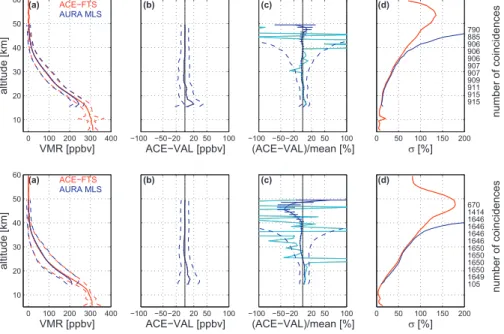
The latitudinal dependence of the ACE-FTS–MLS differences is seen in Fig.4. In general the results are similar for the five bands, with mean absolute differences better than 10 ppbv between 15 and 50 km, and better than 5 ppbv above 20 km, with the

ACPD

Full Screen / Esc

Printer-friendly Version Interactive Discussion

EGU

exception of a few of the lowest altitudes seen in the tropics (30◦_S–30◦_{N) and}

mid-latitudes (30◦_–60◦_{). The ACE-FTS high bias (better than +10% relative deviation from}

the mean, except for the lowermost altitudes in the tropics) and low bias (except for the uppermost altitudes in the 30◦_–60◦_{N and 60}◦_–90◦_{N) persist below and above 24 km,}

respectively.

5

4.3 MIPAS

The Michelson Interferometer for Passive Atmospheric Sounding (MIPAS) is an in-frared limb-sounding Fourier transform interferometer on board Envisat, launched in March 2002 (Fischer et al.,2007). It acquires spectra over the range 685–2410 cm−1

(14.5–4.1µm), which includes the vibration-rotation bands of many molecules of

in-10

terest. It is capable of measuring continuously around an orbit in both day and night, and complete pole-to-pole coverage is obtained in 24 h. From July 2002 until March 2004, MIPAS was operated at full spectral resolution (0.025 cm−1) with a nominal limb-scanning sequence of 17 steps from 68–6 km with 3 km tangent height spacing in the troposphere and stratosphere, generating complete profiles spaced approximately

ev-15

ery 500 km along the orbit. However, in March 2004 operations were suspended fol-lowing problems with the interferometer slide mechanism. Operations were resumed in January 2005 with a 35% duty cycle and reduced spectral resolution (0.0625 cm−1_).

In this section, we describe comparisons between ACE-FTS and MIPAS N₂O products from the full-resolution mission generated by the ESA operational processor version

20

4.62 (hereafter referred to as MIPAS ESA) and by the Institut f ¨ur Meteorologie und Klimaforschung (IMK) / Instituto de Astrof´ısica de Andaluc´ıa (IAA) scientific processor version 9 (hereafter referred to as MIPAS IMK-IAA). Negative values in the ESA data product are set to zero; at altitudes above ∼40 km, where the N2O VMR is very small,

this can result in a high bias of ESA N₂O relative to IMK-IAA N₂O.

ACPD

Full Screen / Esc

Printer-friendly Version Interactive Discussion

EGU

4.3.1 MIPAS ESA N₂O

For the high-resolution mission, ESA has processed pressure, temperature, and six species (H₂O, O₃, HNO₃, CH₄, N₂O and NO₂). The algorithm used for the level 2 analysis is based on the Optimised Retrieval Model (ORM) (Raspollini et al., 2006;

Ridolfi et al.,2000) and uses microwindows at 1233.275–1236.275 cm−1and 1272.05–

5

1275.05 cm−1 for the N₂O retrievals. Here, MIPAS v4.62 N₂O data are compared with ACE-FTS version 2.2 data from 21 February 2004 to 26 March 2004. The vertical resolution of the MIPAS VMR profiles is 3–4 km and the horizontal resolution is 300– 500 km along-track (Vigouroux et al.,2007). During the first five months of the ACE mission, only sunsets were measured because of problems with spacecraft pointing at

10

sunrise. Therefore the latitude coverage for this comparison is limited to 20◦N–85◦N for the selected coincidence criteria of ±6 h and 300 km. The intercomparison has been done including all the matching pairs of measurements available in the test period, which yields 141 coincidences (with single counting of profiles). For both ACE-FTS and MIPAS ESA, only profiles associated with successful pressure, temperature and

15

target species retrievals have been considered.

As far as MIPAS ESA errors are concerned, we refer, in general, to the ESA level 2 products for the random error due to propagation of the instru-ment noise through the retrieval (see Piccolo and Dudhia (2007)), and to re-sults of the analysis carried out at University of Oxford (see data available at

20

http://www-atm.physics.ox.ac.uk/group/mipas/err) for the systematic error. Some of

the components, listed in the Oxford University data set as systematic error on the in-dividual profiles, show a random variability over the longer time-scales involved when averaging different MIPAS scans and/or orbits and tend to contribute to the standard deviation of the mean difference rather than to the bias. Taking this into account, for

25

this intercomparison with ACE-FTS, we have considered the error contribution due to propagation of pressure and temperature random covariance into the retrieval of key species VMR (taken from the Oxford University data set) as a randomly variable

ACPD

Full Screen / Esc

Printer-friendly Version Interactive Discussion

EGU

component and combined it with the measurement noise – using the root-sum-square method – to obtain MIPAS ESA random error.

Figure 5shows the results of the comparison. The mean absolute difference is as large as −38 ppbv at 6.5 km, within ±17 ppbv from 8–60 km, within ±10 ppbv above 15 km, with typical values of ±2 ppbv, particularly above 20 km. ACE-FTS has a low

5

bias relative to MIPAS ESA between 6–10 km, 15–20 km, and 32–60 km. For this comparison, the mean relative difference and the relative deviation from the mean are similar and within ±10% (±4 typical) from 8 to 26 km, then increasing steadily to values greater than -20% in the relative deviation from the mean above 35 km, where the standard deviations on the mean ACE-FTS and MIPAS profiles are also large.

10

The pronounced low bias of ACE-FTS compared to MIPAS ESA at higher altitudes is probably due to the negative values in the ESA data product being set to zero.

4.3.2 MIPAS IMK-IAA N₂O

The strategy and characteristics of the MIPAS IMK-IAA N₂O vertical profile retrievals are described byGlatthor et al.(2005). N₂O is retrieved jointly with CH₄from its infrared

15

emission lines in the spectral range from 1230 to 1305 cm−1_{. Spectroscopic data are}

taken from the HITRAN 2004 database (Rothman et al.,2005). The vertical resolution in the case of mid-latitude profiles is about 3–4 km up to altitudes around 40 km, and increases to 6 km at an altitude of 50 km. The noise error is equal to or less than 5% up to 50 km. The systematic errors are within 10% up to 30 km and increase up to 30%

20

above 30 km.

Here we compare N₂O profiles from ACE-FTS sunset observations with MIPAS IMK-IAA measurements from 21 February 2004 until 25 March 2004, when the MI-PAS full-resolution mode data ended. For these comparisons, we used as coinci-dence criteria a maximum time difference of 9 h, a maximum tangent point difference

25

of 800 km, and a maximum potential vorticity (PV) difference of 3×10−6_km2_kg−1_s−1

on the 475 K potential temperature level. Over all matches, this resulted in a mean distance of 296 km (±154 km), a mean PV difference of −0.007 ×10−6_km2_kg−1_s−1

ACPD

Full Screen / Esc

Printer-friendly Version Interactive Discussion

EGU

(±1.49×10−6_km2_kg−1_s−1_{) and a mean time difference of −0.2 h. The distribution of}

the time differences is bi-modal since MIPAS measurements are either at around late morning or early night, while the ACE-FTS observations used here are made during sunset. Thus, for nighttime MIPAS observations, the time difference (MIPAS – ACE) is 4–5 h, while in the case of MIPAS daytime measurements it is about −6 to −8 h.

5

Since N₂O shows no diurnal cycle in the sounded altitude range and since there is no significant difference between the daytime and nighttime comparisons, in the following we show the mean differences for day- and night-time matches together, as was done for the comparisons with the MIPAS ESA product.

Nevertheless, stratospheric N₂O profiles are affected by the subsidence inside

10

the Arctic polar vortex. Thus, in Fig. 6 we show separately the results of the comparisons outside (372 coincidences with single counting of profiles) and inside (114 coincidences) the polar vortex. We determined the matches outside (inside) the vortex by values of PV of <30×10−6 _(>35×10−6_{) km}2

kg−1s−1 on the 475 K potential temperature level. Both instruments nicely detect the typical subsidence of inner

vor-15

tex N₂O profiles compared to extra-vortex measurements. In general, the differences between MIPAS and ACE-FTS are similar irrespective of their position relative to the vortex. Over the entire 11–60 km altitude range of the comparison, the mean absolute differences are typically −3 ppbv (maximum difference −30 ppbv) inside the vortex and −5 ppbv (maximum difference −42 ppbv) outside. The corresponding relative

devia-20

tions from the mean are typically −6% (maximum −43%) inside the vortex, and +3% (maximum +48%) outside, with oscillations about 0 as seen in Fig.6c. Below about 26 km, ACE-FTS is smaller than MIPAS both outside and inside the vortex. The abso-lute differences are largest below about 18 km, which can be attributed to a high bias in the MIPAS data that has also been observed in other comparisons. However, the

25

reason for the bump (+20%) at 30 km in the extra-vortex observations is an open issue. The relative deviations from the mean are largest at the highest altitudes, as expected given the very small N₂O VMRs in that region. The best agreement between ACE-FTS and MIPAS, taking into account both the mean absolute differences and the relative

de-ACPD

Full Screen / Esc

Printer-friendly Version Interactive Discussion

EGU

viations from the mean, is seen between 18 and 35 km. In this region, on average, the mean absolute differences are −1 ppbv (−6 ppbv maximum) and −3 ppbv (−14 ppbv maximum) inside and outside the vortex, respectively, while the corresponding relative deviations from the mean are −5% (−13% maximum) and −1% (+22% maximum) in-side and outin-side, respectively. It is also interesting to note the very similar variability

5

observed by ACE-FTS and MIPAS, as seen in the standard deviations in Fig.6d.

5 Comparisons with aircraft and balloon-borne measurements

5.1 ASUR

The Airborne Submillimeter wave Radiometer from the University of Bremen is a pas-sive heterodyne radiometer operating in the frequency range from 604.3 to 662.3 GHz

10

(von Koenig et al., 2000), which measures a number of species, including N₂O, O₃,

HNO₃, and CO. Stratospheric N₂O measurements obtained with the Acousto Optical Spectrometer are used in this study. The total bandwidth of the spectrometer is 1.5 GHz and its resolution is 1.27 MHz; N₂O is retrieved using the 652.833 GHz line. This re-ceiver is designed to carry out measurements from a high-altitude research aircraft in

15

order to avoid signal absorption by tropospheric water vapor during the observations. ASUR is an upward-looking instrument at a stabilized constant zenith angle of 78◦. The receiver measures thermal emissions from the rotational lines of the target molecule. The shape of the pressure-broadened lines is related to the vertical distribution of the trace gas. The measured spectra are integrated up to 150 s, which leads to a horizontal

20

resolution of about 30 km along the flight path. The vertical profiles of the molecule are retrieved on an equidistant altitude grid of 2-km spacing using the optimal estimation method (Rodgers,2000). The vertical resolution of the N₂O measurements is 8–16 km and the vertical range is 18 to 46 km. The precision of a typical single measurement is 10 ppbv and the accuracy is 15% or 30 ppbv, whichever is larger, including systematic

25

uncertainties. Details about the measurement technique and retrieval theory can be found inKuttippurath(2005).

ACPD

Full Screen / Esc

Printer-friendly Version Interactive Discussion

EGU

The ASUR N₂O measurements used here were performed during the Polar Aura Validation Experiment (PAVE) campaign (http://www.espo.nasa.gov/ave-polar/). Data from five selected ASUR measurement flights (on 24, 25, and 31 January 2005, and 2 and 7 February 2005) during the campaign are compared with ACE-FTS occultations between 60◦_{N and 70}◦_{N. ASUR measurements within 1000 km and ±12 h of the} satel-5

lite observations were selected, yielding seven ACE-FTS profiles, 15 ASUR profiles, and 17 co-located observation pairs. Because the vertical resolution of the ASUR pro-files is lower than that of the satellite propro-files, the ACE-FTS N₂O vertical profiles were convolved with the ASUR N₂O averaging kernels, and compared on the 2-km ASUR altitude grid.

10

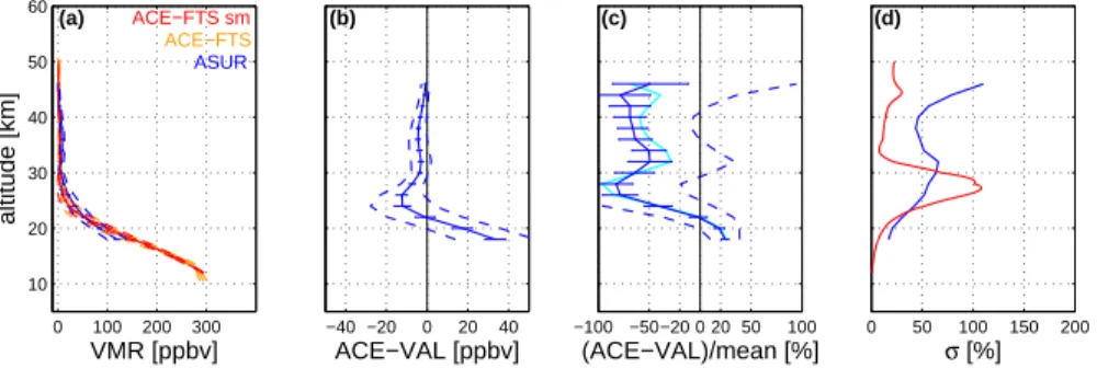
Figure 7 shows the results from the comparison. The best agreement between the ASUR and ACE-FTS mean absolute difference profiles is between 30 and 46 km, where they agree to within −4.5 ppbv and on average, to within −3 ppbv. Between 18 and 30 km, the maximum difference is +33 ppbv and typical differences are within ±10 ppbv. The ACE-FTS profiles are consistently smaller than ASUR above 22 km, and

15

larger for the comparisons at 18 and 20 km. The relative deviations from the mean are large, reaching a maximum of +82% at 28 km. In general, the ACE-FTS profiles are in reasonable agreement with the ASUR profiles, as the differences are well within the estimated accuracy of ASUR N₂O, i.e., 30 ppbv.

5.2 SPIRALE

20

SPIRALE (Spectroscopie Infra-Rouge d’Absorption par Lasers Embarqu ´es) is a balloon-borne tunable diode laser absorption spectrometer operated by LPCE (Lab-oratoire de Physique et Chimie de L’Environment, CNRS-Universit ´e d’Orl ´eans)

(Moreau et al.,2005), which has participated in several European satellite validation

campaigns for Odin and Envisat. It can perform simultaneous in situ measurements

25

of about ten chemical species from about 10 to 35 km height, with a high-frequency sampling (∼1 Hz), thus enabling a vertical resolution of a few meters depending on the ascent rate of the balloon. It has six tunable diode lasers that emit in the mid-infrared

ACPD

Full Screen / Esc

Printer-friendly Version Interactive Discussion

EGU

from 3 to 8µm, with beams injected into a multi-pass Heriott cell located under the

gondola and largely exposed to ambient air. The 3.5-m-long cell is deployed during the ascent when the pressure is less than 300 hPa, and provides a total optical path between the two cell mirrors of 430.78 m. N₂O concentrations are retrieved from direct infrared absorption of the ro-vibrational line at 1275.49 cm−1_{, by fitting experimental} 5

spectra with spectra calculated using HITRAN 2004 database (Rothman et al.,2005). Measurements of pressure (by two calibrated and temperature-regulated capacitance manometers) and temperature (by two probes made of resistive platinum wire) aboard the gondola allow conversion of the measured number densities into VMRs. Uncer-tainties on these parameters and on the spectroscopic data (essentially molecular

10

line strength and pressure broadening coefficients) are negligible relative to the other sources of error. The uncertainties in the VMRs have been assessed by taking into account random and systematic errors, and combining them as the square root of their quadratic sum. The random errors (fluctuations of the laser background emission signal and signal-to-noise ratio) and the systematic errors (laser line width and

non-15

linearity of the detector) are very low, resulting in an estimated total uncertainty of 3% for N₂O volume mixing ratios above 3 ppbv (i.e., at altitudes<26 km) and 6% for mixing

ratios below 3 ppbv (>26 km).

The SPIRALE balloon flight occurred on 20 January 2006 between 17:46 UT and 19:47 UT, with a vertical profile obtained during ascent between 13.2 and 27.2 km.

20

The measurement position remained rather constant, with the balloon mean location at 67.6±0.2◦N and 21.55±0.20◦E. The comparison is made with ACE-FTS sunrise oc-cultation sr13151, which occurred 13 hours later (on 21 January 2006 at 08:00 UT) and located at 64.28◦_{N and 21.56}◦_{E, i.e., 413 km away from SPIRALE. Using the}

MI-MOSA (Mod ´elisation Isentrope du transport M ´eso- ´echelle de l’Ozone Stratosph ´erique

25

par Advection) contour advection model (Hauchecorne et al.,2002), PV maps in the region of both measurements have been calculated each hour between 17:00 UT on 20 January and 08:00 UT on 21 January on isentropic surfaces, every 50 K from 350 K to 800 K (corresponding to 12.8–30 km height). These PV fields indicated that SPIRALE

ACPD

Full Screen / Esc

Printer-friendly Version Interactive Discussion

EGU

and ACE-FTS sampled similar air masses within the polar vortex, with PV agreement better than 10%.

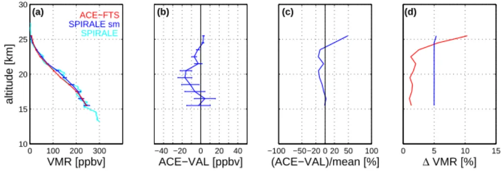
Given the very high vertical resolution (on the order of meters) of the SPIRALE N₂O profile, it was smoothed by a triangular weighting function of 3 km at the base and interpolated onto the ACE-FTS 1-km grid as discussed in Sect. 3. This smoothing

5

truncated the bottom and the top of the SPIRALE profile by 1.5 km. Figure8 shows that the ACE-FTS and SPIRALE N₂O profiles agree to within 17 ppbv (and are typically within ±6) in the 15 to 26 km altitude range, with relative differences between −15% and +19% (and ±5 on average) except at the highest altitude, where the difference increases to +49%. ACE-FTS is consistently smaller than SPIRALE between 17 and

10

24 km. 5.3 FIRS-2

FIRS-2 (Far-InfraRed Spectrometer-2) is a balloon-borne Fourier transform infrared spectrometer designed and built at the Smithsonian Astrophysical Observatory. It has contributed to numerous previous satellite validation efforts (e.g., Roche et al.,

15

1996; Jucks et al., 2002; Nakajima et al., 2002; Canty et al., 2006). FIRS-2

de-tects atmospheric thermal emission in limb-viewing mode from approximately 7 to 120µm at a spectral resolution of 0.004 cm−1 _{(Johnson et al.,1995). Vertical profiles}

of about 30 trace gases are retrieved from the float altitude (typically 38 km) down to the tropopause using a nonlinear Levenberg-Marquardt least-squares algorithm, with

20

pressure and temperature profiles derived from the 15µm band of CO2. Uncertainty

estimates for FIRS-2 contain random retrieval error from spectral noise and systematic components from errors in atmospheric temperature and pointing angle (Johnson et

al.,1995;Jucks et al.,2002). N₂O profiles are retrieved using theν2band between 550

and 600 cm−1_. 25

ACE-FTS is compared with the N₂O profile obtained during a FIRS-2 balloon flight from Esrange, Sweden on 24 January 2007. The average location of the flight was 67.27◦_{N, 27.29}◦_{E, with some smearing of the longitude footprint as FIRS-2 was}

ob-ACPD

Full Screen / Esc

Printer-friendly Version Interactive Discussion

EGU

serving to the east. The data were recorded before local solar noon, at 10:11 UT, with a solar zenith angle of 86.6◦_{. The float altitude was just under 28 km, limiting the}

maximum measurement altitude to 31 km. The 1σ error on the the measured N₂O VMR varied from 5–14% between 13 and 23 km, and increased steadily above 23 km to 117% at 31 km. The closest ACE-FTS occultation was sr18561, obtained on 23

5

January 2007, at 08:25 UT, 64.70◦_{N, 15.02}◦_{E, placing it 481 km away from the}

loca-tion of the balloon flight, and almost 26 h earlier. The FIRS-2 footprint was inside the vortex, while the ACE-FTS occultation was nearer the vortex edge. The FIRS-2 N₂O profile, reported on a 1-km grid, was interpolated onto the ACE-FTS 1-km grid. Fig-ure9 _{shows the results of the comparison. The absolute differences vary from −12} 10

to +30 ppbv over the full altitude range of 13–31 km, with typical values of of +8 and +5 ppbv below and above 20 km, respectively. The largest absolute differences are be-low 15 km, where FIRS-2 reported be-low values of N₂O, although the relative differences have maxima at 25 and 28 km (_{>±100%). It is possible that FIRS-2 is seeing} subsi-dence within the vortex. Below 20 km, the relative differences are between −6% and

15

+17%, but they increase significantly above 20 km. ACE-FTS has a low bias relative to FIRS-2 between 11 and 13 km, and between 27 and 30 km.

6 Comparisons with ground-based FTIR measurements

In addition to the vertical profile comparisons described above, ACE-FTS N₂O mea-surements have been compared with partial columns retrieved from solar absorption

20

spectra recorded by ground-based Fourier transform infrared spectrometers. Twelve such instruments participated in this study; all are at stations of the Network for the Detection of Atmospheric Composition Change (NDACC) (Kurylo and Zander,2000) and make regular measurements of a suite of tropospheric and stratospheric species. Many have previously provided data for validation of N₂O measurements by satellite

25

instruments, such as ILAS (Wood et al.,2002), ILAS-II (Griesfeller et al.,2006), SCIA-MACHY (Dils et al.,2006), and MIPAS (Vigouroux et al.,2007). Table2lists the stations

ACPD

Full Screen / Esc

Printer-friendly Version Interactive Discussion

EGU

involved, including their location, the instrument type and spectral resolution, and the retrieval code and microwindows used to retrieve N₂O. More information about the in-struments, the retrieval methodologies, and the measurements made at each of these sites can be found in the references provided in Table 2. The participating stations cover latitudes from 77.8◦_{S to 78.9}◦_{N, and provide measurements from the subtropics} 5

to the polar regions in both hemispheres.

The FTIR measurements require clear-sky conditions, but are made year-round, thus providing good temporal coverage for comparisons with ACE-FTS. The data used here were analyzed using either the SFIT2 retrieval code (Pougatchev and

Rins-land, 1995; Pougatchev et al., 1995; Rinsland et al., 1998) or PROFFIT92 (Hase,

10

2000).Hase et al.(2004) found that N₂O VMR profiles retrieved using these two codes

showed very good agreement, with total columns agreeing to within 1%. Both algo-rithms employ the optimal estimation method (Rodgers,2000) to retrieve vertical pro-files from a statistical weighting between a priori information and the high-resolution spectral measurements.Barbe and Marche(1985) andSussmann and Sch ¨afer(1997)

15

also showed how information on the vertical distribution of N₂O could be derived from ground-based infrared spectra. Averaging kernels calculated as part of the optimal esti-mation analysis quantify the inforesti-mation content of the retrievals, and can be convolved with the ACE-FTS profiles, which have higher vertical resolution. For N₂O, there are typically 3–4 Degrees Of Freedom for Signal (DOFS, equal to the trace of the averaging

20

kernel matrix) in the total column, and 1–2 in the altitude range coincident with ACE-FTS measurements. Given this coarse vertical resolution, we compare partial columns rather than profiles. All participating sites used microwindows in the 2480–2485 cm−1 region for the N₂O retrievals, with several sites also including microwindows between 2526 and 2541 cm−1_{; these are listed in Table2. All sites used spectroscopic data from} 25

HITRAN2004, with the exception of Harestua, which used HITRAN 2000, and Kiruna and Iza ˜na, which used HITRAN 2000 + official updates. Recent analysis using Kiruna data coincident with ACE-FTS have shown that N₂O columns retrieved with HITRAN 2000 are 1.3% larger than those retrieved with HITRAN 2004, so the Harestua, Kiruna,