Atmos. Chem. Phys., 8, 3529–3562, 2008 www.atmos-chem-phys.net/8/3529/2008/ © Author(s) 2008. This work is distributed under the Creative Commons Attribution 3.0 License.
Atmospheric
Chemistry
and Physics
Validation of HNO
3
, ClONO
2
, and N
2
O
5
from the Atmospheric
Chemistry Experiment Fourier Transform Spectrometer
(ACE-FTS)
M. A. Wolff1, T. Kerzenmacher1, K. Strong1, K. A. Walker1,2, M. Toohey1, E. Dupuy2, P. F. Bernath2,3, C. D. Boone2, S. Brohede4, V. Catoire5, T. von Clarmann6, M. Coffey7, W. H. Daffer8, M. De Mazi`ere9, P. Duchatelet10, N. Glatthor6, D. W. T. Griffith11, J. Hannigan7, F. Hase6, M. H¨opfner6, N. Huret5, N. Jones11, K. Jucks12, A. Kagawa13, 14,
Y. Kasai14, I. Kramer6, H. K ¨ullmann15, J. Kuttippurath15,*, E. Mahieu10, G. Manney16,17, C. T. McElroy18, C. McLinden18, Y. M´ebarki5, S. Mikuteit6, D. Murtagh4, C. Piccolo19, P. Raspollini20, M. Ridolfi21, R. Ruhnke6, M. Santee16, C. Senten9, D. Smale22, C. T´etard23, J. Urban4, and S. Wood22
1Department of Physics, University of Toronto, Toronto, Ontario, Canada 2Department of Chemistry, University of Waterloo, Waterloo, Ontario, Canada 3Department of Chemistry, University of York, York, UK
4Department of Radio and Space Science, Chalmers University of Technology, Gothenburg, Sweden 5Laboratoire de Physique et Chimie de L’Environment CNRS – Universit´e d’Orl´eans, Orl´eans, France
6Forschungzentrum Karlsruhe and Univ. of Karlsruhe, Institute for Meteorology and Climate Research, Karlsruhe, Germany 7National Center for Atmospheric Research (NCAR), Boulder, CO, USA
8Columbus Technologies Inc., Pasadena, CA, USA 9Belgian Institute for Space Aeronomy, Brussels, Belgium
10Institute of Astrophysics and Geophysics, University of Li`ege, Li`ege, Belgium 11School of Chemistry, University of Wollongong, Wollongong, Australia 12Harvard-Smithsonian Center for Astrophysics, Cambridge, MA, USA 13Fujitsu FIP Corporation, Tokyo, Japan
14Environmental Sensing and Network Group, National Institute of Information and Communications Technology (NICT), Tokyo, Japan
15Institute of Environmental Physics, University of Bremen, Bremen, Germany 16Jet Propulsion Laboratory, California Institute of Technology, Pasadena, CA, USA 17New Mexico Institute of Mining and Technology, Socorro, NM, USA
18Environment Canada, Toronto, Ontario, Canada
19Atmospheric, Oceanic and Planetary Physics, University of Oxford, Oxford, UK
20Institute of Applied Physics “Nello Carrara”, National Research Center (CNR), Firenze, Italy 21Dipartimento di Chimica Fisica e Inorganica, Universit`a di Bologna, Bologna, Italy
22National Institute of Water and Atmospheric Research Ltd., Central Otago, New Zealand
23Laboratoire d’Optique Atmosph´erique, Universit´e des Sciences et Technologies de Lille, Villeneuve d’Ascq, France *now at: LMD/CNRS Ecole polytechnique, Palaiseau Cedex, France
Received: 4 December 2007 – Published in Atmos. Chem. Phys. Discuss.: 11 December 2007 Revised: 5 June 2008 – Accepted: 5 June 2008 – Published: 7 July 2008
Correspondence to: M. A. Wolff
Abstract. The Atmospheric Chemistry Experiment (ACE) satellite was launched on 12 August 2003. Its two instru-ments measure vertical profiles of over 30 atmospheric trace gases by analyzing solar occultation spectra in the ultra-violet/visible and infrared wavelength regions. The reser-voir gases HNO3, ClONO2, and N2O5are three of the key species provided by the primary instrument, the ACE Fourier Transform Spectrometer (ACE-FTS). This paper describes the ACE-FTS version 2.2 data products, including the N2O5 update, for the three species and presents validation com-parisons with available observations. We have compared volume mixing ratio (VMR) profiles of HNO3, ClONO2, and N2O5with measurements by other satellite instruments (SMR, MLS, MIPAS), aircraft measurements (ASUR), and single balloon-flights (SPIRALE, FIRS-2). Partial columns of HNO3 and ClONO2 were also compared with measure-ments by ground-based Fourier Transform Infrared (FTIR) spectrometers. Overall the quality of the ACE-FTS v2.2 HNO3VMR profiles is good from 18 to 35 km. For the statis-tical satellite comparisons, the mean absolute differences are generally within ±1 ppbv (±20%) from 18 to 35 km. For MI-PAS and MLS comparisons only, mean relative differences lie within ±10% between 10 and 36 km. ACE-FTS HNO3 partial columns (∼15–30 km) show a slight negative bias of
−1.3% relative to the ground-based FTIRs at latitudes rang-ing from 77.8◦S–76.5◦N. Good agreement between ACE-FTS ClONO2and MIPAS, using the Institut f¨ur Meteorolo-gie und Klimaforschung and Instituto de Astrof´ısica de An-daluc´ıa (IMK-IAA) data processor is seen. Mean absolute differences are typically within ±0.01 ppbv between 16 and 27 km and less than +0.09 ppbv between 27 and 34 km. The ClONO2partial column comparisons show varying degrees of agreement, depending on the location and the quality of the FTIR measurements. Good agreement was found for the comparisons with the midlatitude Jungfraujoch partial columns for which the mean relative difference is 4.7%. ACE-FTS N2O5has a low bias relative to MIPAS IMK-IAA, reaching −0.25 ppbv at the altitude of the N2O5 maximum (around 30 km). Mean absolute differences at lower altitudes (16–27 km) are typically −0.05 ppbv for MIPAS nighttime and ±0.02 ppbv for MIPAS daytime measurements.
1 Introduction
This is one of two papers describing the validation of NOy species measured by the Atmospheric Chemistry Experiment (ACE) through comparisons with coincident measurements. The total reactive nitrogen, or NOy, family consists of NOx (NO + NO2) + all oxidized nitrogen species:
[NOy] = [NO] + [NO2] + [NO3] + [HNO3] + [HNO4]
+ [ClONO2] + [BrONO2] +2[N2O5]. (1) The ACE-Fourier Transform Spectrometer (ACE-FTS) mea-sures all of these species, with the exception of NO3 and
BrONO2(Bernath et al., 2005), while the ACE-Measurement of Aerosol Extinction in the Stratosphere and Troposphere Retrieved by Occultation (ACE-MAESTRO) also measures NO2(McElroy et al., 2007). The species NO, NO2, HNO3, ClONO2, and N2O5are five of the 14 primary target species for the ACE mission, while HNO4is a research product. In this study, the quality of the ACE-FTS version 2.2 nitric acid (HNO3), chlorine nitrate (ClONO2), and ACE-FTS version 2.2 dinitrogen pentoxide (N2O5) update is assessed prior to its public release. A companion paper by Kerzenmacher et al. (2008) provides an assessment of the ACE-FTS v2.2 nitric oxide (NO) and nitrogen dioxide (NO2), and of the ACE-MAESTRO v1.2 NO2. Validation of ACE-FTS v2.2 mea-surements of nitrous oxide (N2O), the source gas for NOy, is discussed by Strong et al. (2008).
The three molecules HNO3, ClONO2, and N2O5 are im-portant reservoir species for nitrogen and chlorine in the stratosphere and therefore play an important role in strato-spheric ozone chemistry. They can sequester the more re-active NOx species, thereby reducing ozone destruction via fast catalytic cycles (Solomon, 1999; Brasseur and Solomon, 2005). NOx/NOy partitioning is largely determined by ozone and aerosol concentrations (e.g. Salawitch et al., 1994; Solomon et al., 1996). HNO3is the dominant form of NOy in the lower stratosphere, and is produced from NOxby the reaction:
NO2+OH + M → HNO3+M (R1)
where M is a third body that remains unchanged under the reaction. HNO3is chemically destroyed by photolysis and oxidation by OH:
HNO3+hν →OH + NO2 (R2)
HNO3+OH → NO3+H2O. (R3)
Both processes make comparable contributions to HNO3loss in the lower stratosphere. At higher altitudes, Reaction (R3) becomes gradually more important and dominates the HNO3 loss mechanisms in the upper stratosphere (Dessler, 2000).
ClONO2is also produced from NOxby reaction with ClO:
ClO + NO2+M → ClONO2+M (R4)
and is photolyzed at ultraviolet wavelengths to create either Cl + NO3, or ClO + NO2.
N2O5is created through the reaction:
NO2+NO3+M → N2O5+M. (R5)
Because of the extremely low abundances of NO3during the day, this process occurs at night (Dessler, 2000). N2O5is mainly destroyed by photolysis (more than 90%) and col-lisional decomposition, to generate NO3 and either NO2or NO+O.
M. A. Wolff et al.: Validation of HNO3, ClONO2and N2O5from ACE-FTS 3531 During polar winter, the conversion of NOx and ClO to
HNO3, ClONO2, and N2O5reduces the chemical destruction of ozone. However, in the presence of polar stratospheric clouds (PSCs), ClONO2 and N2O5 can undergo heteroge-neous reactions with H2O and HCl to create HNO3and re-lease chlorine into chemically active forms. HNO3 can, in turn, be removed from the gas phase through sequestration on the PSCs, and subsequently lost through sedimentation of large PSC particles. This process of denitrification ef-fectively removes NOy from the stratosphere, thereby sup-pressing Reaction (R4), and redistributes it to lower altitudes where the PSCs evaporate (e.g. Toon et al., 1986; Waibel et al., 1999). Hydrolysis of N2O5 can also occur on sul-phuric acid aerosols, thereby affecting both HNO3 concen-trations and the ozone budget at mid-latitudes (Hofmann and Solomon, 1989).
Of the three species that are the focus of this work, HNO3 has been the most widely measured. The first measure-ments of HNO3 in the stratosphere were made by Murcray et al. (1968), and were followed by the first space-based measurements made by the Limb Infrared Monitor of the Stratosphere (LIMS) on Nimbus 7 (Gille and Russell, 1984; Gille et al., 1984). Regular ground-based Fourier trans-form infrared spectrometer (FTIR) measurements of HNO3 were started in 1980 at the National Solar Observatory Mc-Math solar telescope facility on Kitt Peak, Arizona, USA and in 1986 at the International Scientific Station of the Jungfraujoch (ISSJ) in the Swiss Alps (Rinsland et al., 1991). Since then, other stations have performed continuous FTIR measurements of HNO3, most of them as part of the Net-work for the Detection of Atmospheric Composition Change (NDACC, http://www.ndacc.org). HNO3was measured dur-ing a series of Space Shuttle missions by the Atmospheric Trace MOlecule Spectroscopy (ATMOS) instrument, flown four times between 1985 and 1994 (Abrams et al., 1996; Gunson et al., 1996; Irion et al., 2002), by the CRyogenic InfraRed Radiance Instrumentation for Shuttle (CIRRIS 1A) (Bingham et al., 1997) in 1991, and by the CRyogenic In-frared Spectrometers and Telescopes for the Atmosphere (CRISTA) in 1994 (Offermann et al., 1999; Riese et al., 1999). With the launch of the Upper Atmosphere Research Satellite (UARS) in 1991, longer-term global distributions of HNO3were retrieved by the Cryogenic Limb Array Etalon Spectrometer (CLAES) (Roche et al., 1993, 1994; Kumer et al., 1996a), the Improved Stratospheric And Mesospheric Sounder (ISAMS) (Taylor et al., 1993, 1994, 1995), and the Microwave Limb Sounder (MLS) (Santee et al., 1999, 2004; Waters et al., 2006). The latter provides the most extensive HNO3 dataset to date. More recently, the Improved Limb Atmospheric Spectrometer (ILAS) on the Advanced Earth Observing Satellite (ADEOS) (Koike et al., 2000; Irie et al., 2002; Nakajima et al., 2002) and ILAS-II on ADEOS-II (Irie et al., 2006) both measured HNO3using infrared solar occul-tation.
In addition to the ACE-FTS, there are currently four satellite instruments measuring HNO3. The Sub-Millimetre Radiometer (SMR) on Odin has been in orbit since 2001 (Murtagh et al., 2002; Urban et al., 2005), and the Michelson Interferometer for Passive Atmospheric Sounding (MIPAS) on Envisat, since 2002 (Mengistu Tsidu et al., 2005; Stiller et al., 2005; Wang et al., 2007a,b; Fischer et al., 2008). The Aura satellite, launched in 2004, carries another MLS (Wa-ters et al., 2006; Santee et al., 2007) and the HIgh Resolution Dynamics Limb Sounder (HIRDLS) (Gille et al., 2008; Kin-nison et al., 2008). These instruments are described in more detail below, in the context of comparisons with ACE-FTS.
Stratospheric ClONO2 was first measured by Murcray et al. (1979) and Rinsland et al. (1985) using solar infrared absorption spectroscopy from a balloon platform. Zander and Demoulin (1988) reported on the retrieval of ClONO2 column densities from FTIR measurements at the moun-tain station of the Jungfraujoch. Today, many of the FTIRs affiliated with NDACC perform ClONO2 measurements. ClONO2 was measured from space by ATMOS during all four Space Shuttle missions using infrared solar occulta-tion spectroscopy (Zander et al., 1986; Rinsland et al., 1994, 1985, 1996; Zander et al., 1996) and by CRISTA using ob-servations of infrared thermal emission (Offermann et al., 1999; Riese et al., 1999). CLAES was the only instrument on UARS able to detect ClONO2, and it provided global profiles between October 1991 and May 1993 (Mergenthaler et al., 1996). It was followed by ILAS, which measured ClONO2 from October 1996 to June 1997 (Nakajima et al., 2006), pro-viding the first high-latitude coverage, and by ILAS-II from January to October 2003 (Wetzel et al., 2006). Currently, MI-PAS is the only instrument, other than ACE-FTS, which is in orbit and measuring ClONO2; H¨opfner et al. (2007) describe validation of the profiles retrieved using the Institut f¨ur Me-teorologie und Klimaforschung and Instituto de Astrof´ısica de Andaluc´ıa (IMK-IAA) scientific data processor.
Spectroscopic measurements of N2O5 are difficult due to the presence of interfering species and aerosol in the 1240 cm−1band that is typically used for retrievals. The first detection was by King et al. (1976); for a review of early efforts to measure N2O5from the ground and balloons, see Roscoe (1991). Like ClONO2, stratospheric N2O5has been detected from space by ATMOS (Abrams et al., 1996; Gun-son et al., 1996), CRISTA (Riese et al., 1997, 1999), CLAES (Kumer et al., 1996b, 1997), ILAS (Yokota et al., 2002; Os-hchepkov et al., 2006), and ILAS-II (Wetzel et al., 2006). In addition, ISAMS, which operated on UARS from October 1991 to July 1992, detected N2O5using pressure modulated radiometry (Taylor et al., 1993; Smith et al., 1996; Kumer et al., 1997). MIPAS is again the only instrument, other than ACE-FTS, which is currently measuring N2O5 from space (Mengistu Tsidu et al., 2004).
To date, ACE-FTS v2.2 HNO3volume mixing ratio pro-files have been compared with data from the following satellite instruments: MIPAS ESA (Wang et al., 2007a),
MIPAS IMK-IAA (Wang et al., 2007b), Aura-MLS (Froide-vaux et al., 2006; Toohey and Strong, 2007; Santee et al., 2007), and HIRDLS (Kinnison et al., 2008). Addition-ally, they have been compared to balloon-borne measure-ments carried out during the Middle Atmosphere Nitro-gen TRend Assessment (MANTRA) mission (Toohey et al., 2007). Mahieu et al. (2005) compared ACE-FTS v.1.0 ClONO2 with ground-based measurements at northern lat-itudes and ACE-FTS v2.2 ClONO2 profiles have been in-cluded in the validation of MIPAS IMK-IAA data products (H¨opfner et al., 2007).
The objective of this validation exercise is to assess the quality of the current ACE-FTS data (v2.2 with updates for O3, N2O5, and HDO). In this study, we compare the ACE-FTS v2.2 HNO3 and ClONO2data and the ACE-FTS v2.2 N2O5update data through comparisons with coincident mea-surements. The paper is organized as follows. In Sect. 2, the ACE mission and the retrievals of these three species are briefly described. Section 3 summarizes the validation methodology adopted. In Sect. 4, the results of vertical pro-file comparisons with the SMR, MLS, and MIPAS satellite instruments are discussed. Section 5 focuses on the results of comparisons with data from the ASUR (Airborne SUbmil-limeter wave Radiometer) aircraft flights and from the SPI-RALE (SPectroscopie Infra-Rouge d’Absorption par Lasers Embarqu´es) and FIRS-2 (Far-InfraRed Spectrometer-2) bal-loon flights. Partial column comparisons with a network of ground-based FTIRs are presented in Sect. 6. Finally, the re-sults are summarized and conclusions regarding the quality of the HNO3(v2.2), ClONO2(v2.2), and N2O5(v2.2 update) data are given in Sect. 7.
2 ACE-FTS instrument description and data analysis
The Atmospheric Chemistry Experiment was launched on 12 August 2003. ACE is a Canadian-led satellite mission, also known as SCISAT, which carries two instruments, the ACE-FTS (Bernath et al., 2005) and the Measurement of Aerosol Extinction in the Stratosphere and Troposphere Re-trieved by Occultation (ACE-MAESTRO) (McElroy et al., 2007). Both instruments record solar occultation spec-tra, ACE-FTS in the infrared (IR), and MAESTRO in the ultraviolet-visible(vis)-near-IR, from which vertical profiles of atmospheric trace gases, temperature, and atmospheric ex-tinction are retrieved. In addition, a two channel near-IR-vis imager (ACE-IMAGER) provides profiles of atmospheric extinction at 0.525 and 1.02 µm (Gilbert et al., 2007). The SCISAT spacecraft is in a circular orbit at 650-km altitude, with a 74◦inclination angle (Bernath et al., 2005), providing up to 15 sunrise and 15 sunset solar occultations per day. The choice of orbital parameters results in coverage from 85◦S to 85◦N with an annually repeating pattern, and a sam-pling frequency that is greatest over the Arctic and Antarc-tic. The primary scientific objective of the ACE mission is to
understand the chemical and dynamical processes that con-trol the distribution of ozone in the stratosphere and upper troposphere, particularly in the Arctic (Bernath et al., 2005; Bernath, 2006, and references therein).
ACE-FTS measures atmospheric spectra between 750 and 4400 cm−1 (2.2–13 µm) at 0.02 cm−1 resolution (Bernath et al., 2005). Profiles as a function of altitude for pressure, temperature, and over 30 trace gases are retrieved from ACE-FTS measurements. The details of ACE-ACE-FTS data process-ing are described by Boone et al. (2005). Briefly, a non-linear least squares global fitting technique is employed to analyze selected microwindows (0.3–30 cm−1-wide portions of the spectrum containing spectral features for the target molecule). The analysis approach does not employ con-straints from a priori information (i.e. it is not an optimal estimation approach). Prior to performing volume mixing ratio (VMR) retrievals, pressure and temperature, as a func-tion of altitude, are determined through the analysis of CO2 lines in the spectra.
Issues have been identified in some ACE-FTS profiles and these have been flagged as Do Not Use (DNU). A continuously updated list of the DNU profiles and other data issues can be found at https://databace.uwaterloo.ca/ validation/data issues.php.
The ACE-FTS instrument collects measurements every 2 s, which yields a typical altitude sampling of 3–4 km within an occultation, neglecting the effects of refraction that com-press the spacing at low altitudes. Note that this altitude spac-ing can range from 1.5–6 km, dependspac-ing on the geometry of the satellite’s orbit for a given occultation. The actual altitude resolution achievable with the ACE-FTS is limited to about 3–4 km, as a consequence of the instrument’s field-of-view (1.25-mrad-diameter aperture and 650-km altitude). Atmo-spheric quantities are retrieved at the measurement heights. It should be noted that no diurnal corrections have been per-formed for any molecule retrieved from the ACE-FTS ob-servations. For the purpose of generating calculated spectra (i.e. performing forward model calculations), quantities are interpolated from the measurement grid onto a standard 1-km grid using piecewise quadratic interpolation. The com-parisons in this study were performed using the 1-km grid data. Forward model calculations employ the spectroscopic constants and cross section measurements from the HITRAN 2004 line list (Rothman et al., 2005).
The precision of the ACE-FTS v2.2 VMRs is defined as the 1σ statistical fitting errors from the least-squares process, assuming a normal distribution of random errors (Boone et al., 2005). The next ACE-FTS data version will addition-ally account for systematic error contributions, such as the error propagation of the temperature and pressure retrieval errors.
M. A. Wolff et al.: Validation of HNO3, ClONO2and N2O5from ACE-FTS 3533 2.1 HNO3
ACE-FTS v2.2 microwindows for HNO3 lie in the regions from 867–880 cm−1and 1691.5–1728.6 cm−1, used at alti-tudes from 5 to 37 km. A total of 12 microwindows are used in the retrievals. Interferences in the microwindow set in-clude H2O, O3, N2O, CH4, CFC−12, and OCS. The inter-ferers H2O, O3, N2O, and CH4are retrieved simultaneously with HNO3. The OCS VMR profile is fixed to its version 2.2 retrieval result, which is determined prior to the HNO3 retrieval. The contribution of CFC-12 in the microwindows contains no structure, and so is accounted for with the base-line (scale and slope) parameters in the fitting routine.
There is a discrepancy between the spectroscopic con-stants from HITRAN 2004 in the two HNO3 regions (one near 900 cm−1and the other band near 1700 cm−1) used in the ACE-FTS retrievals. Figure 1 shows the difference be-tween using a set of microwindows near 900 cm−1versus a set of microwindows near 1700 cm−1. The profiles shown are an average of 100 occultations. The discrepancy between intensities in the two bands appears to be in the range of 5 to 10%. Note that both regions are required in the retrieval because the region near 900 cm−1 is the only source of in-formation at the lowest altitudes (below 10 km), while the 1700 cm−1-band provides the only information at the highest altitudes (above 35 km). Both regions contribute information for the retrieval between 10 and 35 km. One consequence of this discrepancy is that retrieved HNO3VMR profiles could be noisier than they should be below 12 km. Future versions of ACE-FTS processing will scale the intensities in the band near 1700 cm−1to achieve internal consistency between the two bands.
We have examined the fitting errors for the ACE-FTS HNO3profiles used in the comparisons with MLS (Sect. 4.2), and found that the median value is <5% from 10 to 35 km. 2.2 ClONO2
ACE-FTS v2.2 ClONO2 retrievals employ two microwin-dows containing Q-branches for the molecule. The first microwindow is centered at 780.15 cm−1 with a width of 0.6 cm−1, and is used over the altitude range 12 to 20 km. The second microwindow is centered at 1292.6 cm−1 with a width of 1.6 cm−1, and extends over the altitude range 18 to 35 km. Interferences in the microwindows include 12CH
4, 13CH4, CH3D, 14N162 O, 14N15N16O, 15N14N16O, H2O, HDO, HNO3, 16O12C18O, 16O12C17O, 16O13C18O, O3, and a minor contribution from H2O2. Interfering species retrieved are O3, HNO3, CH4, and N2O. A single profile is used for all isotopologues of CH4and a single profile is used for all isotopologues of N2O, even though different isotopo-logues of a molecule can have different VMR profiles. The H2O and HDO VMR profiles are fixed to their version 2.2 retrieval results (determined prior to the ClONO2retrieval). The CO2isotopologues use the VMR profile associated with
M. A. Wolff et al.: Validation of HNO3, ClONO2and N2O5from ACE-FTS 29
Fig. 1. Comparison of ACE-FTS HNO3profiles using two
dif-ferent sets of microwindows. Left panel: Retrieved HNO3mean
VMR profiles (averaged over 100 profiles) using the 900 cm−1and
1700 cm−1wavenumber regions. Right panel: Relative differences
calculated as [HNO3(900)–HNO3(1700)]/HNO3(900) as
percent-age.
Fig. 1. Comparison of ACE-FTS HNO3 profiles using two
dif-ferent sets of microwindows. Left panel: Retrieved HNO3mean
VMR profiles (averaged over 100 profiles) using the 900 cm−1and 1700 cm−1wavenumber regions. Right panel: Relative differences calculated as [HNO3(900)–HNO3(1700)]/HNO3(900) as
percent-age.
the main isotopologue of CO2. The VMR profile for H2O2 is fixed to a standard profile taken from the ATMOS ex-periment, sufficiently accurate for this very weak interfer-ence. The microwindow providing information at low alti-tudes (centered at 780.15 cm−1) has a relatively poor signal-to-noise ratio in the ACE-FTS spectra, 40:1 as compared to 350:1 for the microwindow centered at 1292.6 cm−1. Thus, noise on the retrieved VMR profile increases significantly below 18 km. The median fitting errors of the ACE-FTS ClONO2profiles (from the same group of profiles as used for the examination of HNO3fitting errors) are ∼40% at 14 km, below 10% from 20 to 30 km, and increasing to ∼20% at 35 km.
2.3 N2O5
The spectral region analyzed for N2O5 retrievals ranges from 1210 to 1270 cm−1 and is divided into two windows of width 30 cm−1 each. The altitude range for the re-trieval is from 15 to 40 km. Interferences in the spectral region include12CH4,13CH4, CH3D,14N162 O,14N15N16O, 15N14N16O, 14N14N18O, 14N14N17O, H16
2 O, H182 O, HDO, HNO3, 16O12C18O, 16O12C17O, O3, COF2, and a minor contribution from H2O2. Single profiles are retrieved for H2O, CO2, CH4, and N2O, neglecting differences in VMR profiles for different isotopologues. HDO, O3, HNO3, and COF2 are fixed to their version 2.2 retrieval results (deter-mined prior to the N2O5retrieval). As described in the pre-vious section, the VMR profile for H2O2is a standard pro-file taken from the ATMOS mission. N2O5uses the broad-est wavenumber range of any molecule retrieved from the ACE-FTS data. During the original ACE-FTS v2.2 N2O5 retrievals, array overflows occurred during the retrieval pro-cess, not significant enough to cause the software to crash or to trigger any obvious strange behaviour in the retrievals (such as bad fitting residuals). The array overflows caused
a minimum in the retrieved N2O5VMR profile near 30 km, which became evident during the validation process. Hence, a new set of retrievals was performed for N2O5using soft-ware with improved memory management to avoid the array overflows. This new data product has been provided as an update to version 2.2. The original v2.2 N2O5data should not be used. The median N2O5fitting errors, again examined for the group of ACE-FTS profiles as used for the MLS com-parisons, are ∼15% at 15 km and 40 km and below 5% from 20 to 35 km.
3 Validation approach
The ACE-FTS dataset used for these comparisons extends from 21 February 2004 (the start of the ACE Science Oper-ations phase) through to 22 May 2007. The coincidence cri-teria were determined for each correlative dataset in consul-tation with the teams involved, while striving for consistency insofar as possible. The location of each ACE occultation is defined as the latitude, longitude and time of the 30-km tan-gent point (calculated geometrically). This value was used in searching for coincidences.
Coincidence criteria used for the satellite comparisons were between ±6 and ±12 h and between 300 and 800 km. Narrower criteria were chosen for MIPAS data products, for which correlative data was only available for a two-month period in early spring 2004 for northern mid- and high-latitudes. For the balloon and aircraft measurements, profiles obtained within ±26 h and 500 km of ACE-FTS were used. Finally, for the ground-based FTIRs, with some exceptions described in Sect. 6, the criteria were chosen as ±24 h and 1000 km to provide a reasonable number of coincidences. The correlative datasets, temporal and spatial coincidence criteria, and number of coincidences are summarized in Ta-ble 1 for the satellite and airborne instruments. TaTa-ble 2 gives information on the FTIR locations and instruments used.
We report all comparisons on the 1-km ACE-FTS altitude grid. Profiles from all but two of the comparison instruments are retrieved on altitude levels and interpolated onto the ACE altitude grid as described below. However, two of the data sets, MLS and MIPAS ESA, are retrieved on pressure lev-els. As recommended by ESA for the use of the MIPAS ESA data product (Ridolfi et al., 2007) comparisons should be done in the pressure domain in order to avoid additional errors introduced by the pressure to altitude transformation. To minimize such errors and at the same time provide consis-tency with the other comparisons, we performed the follow-ing procedure. The VMR profiles of the pressure-gridded comparison instruments were interpolated in log(p) to the pressure levels of ACE-FTS, which correspond to simulta-neously retrieved ACE-FTS altitude levels. Using this ap-proach, the comparisons, shown for MLS and MIPAS ESA, are performed in the pressure domain, although in the plots they are presented on altitude levels.
Differences in vertical resolution can influence compar-isons, so these have been taken into account in this study. All the satellite instruments and the FIRS-2 balloon instrument have vertical resolutions that are similar to those of ACE-FTS. In these cases, no smoothing was applied to the data and the correlative profiles were linearly interpolated onto the 1-km ACE-FTS altitude grid.
For instruments with lower vertical resolution than ACE-FTS (the aircraft-based ASUR instrument and all ground-based FTIRs) the ACE-FTS profiles were degraded using the averaging kernel matrix and the a priori profile of the comparison instrument (Rodgers and Connor, 2003). Par-tial columns were calculated from all FTIR and coincident smoothed ACE-FTS profiles and used in the comparisons. The balloon-borne SPIRALE VMR profile was obtained at significantly higher vertical resolution than ACE-FTS, and so was convolved with triangular functions having full width at the base equal to 3 km and centered at the tangent height of each occultation. This approach simulates the smoothing effect of the 3–4 km ACE-FTS resolution, as discussed by Dupuy et al. (2008). The resulting smoothed profiles were interpolated onto the 1-km ACE-FTS grid. Co-located pairs of VMR profiles from ACE-FTS and each validation exper-iment (referred to as VAL in text and figures below) were identified using the appropriate temporal and spatial coinci-dence criteria. Then the following procedure was applied to the vertical profile measurements used in this assessment, with some modifications for the individual balloon-borne profile comparisons and the FTIR partial column compar-isons (see Sects. 5 and 6 for details).
(a) Calculate the mean profile of the ensemble for ACE-FTS and the mean profile for VAL, along with the standard deviations on each of these two profiles. These mean profiles are plotted as solid lines, with ±1σ as dashed lines, in panel (a) of the comparison figures discussed below. The standard error on the mean, also known as the uncertainty in the mean, is calculated as σ (z)/√N (z), where N (z) is the number of points used to calculate the mean at a particular altitude, and is included as error bars on the lines in panel (a). Note: in some cases, these error bars, as well as those in panels (b) and (c) (see below) may be small and difficult to distinguish. (b) Calculate the profile of the mean absolute difference, ACE-FTS−VAL, and the standard deviation in the distribu-tion of this mean difference (Note that the term absolute, as used in this work, refers to differences between the compared values and not to absolute values in the mathematical sense). To do this, the differences are first calculated for each pair of profiles at each altitude, and then averaged to obtain the mean absolute difference at altitude z:
1abs(z) = 1 N (z) N (z) X i=1 [ACEi(z) −VALi(z)] (2)
where N (z) is the number of coincidences at z, ACEi(z) is the ACE-FTS VMR at z for the ith coincident pair, and
M. A. Wolff et al.: Validation of HNO3, ClONO2and N2O5from ACE-FTS 3535
Table 1. Summary of the correlative datasets used in the statistical and individual profile comparisons with ACE-FTS HNO3, ClONO2, and
N2O5.
Instrument Comparison Comparison Vertical Range Coincidence Number of Species (Retrieval Code) Period Location and Resolution Criteria Coincidences
SMR 2004/02/21 – 85◦S– 18–45 km ±12 h, 1571 HNO3 (Chalmers v2.0) 2006/11/30 86◦N at 1.5–2.0 km 500 km MLS 2004/09/15 – 82◦S– 215–3.2 hPa ±12 h, 7178 HNO3 (v2.2) 2007/05/22 82◦N at 3.5–5.5 km ±1◦lat., ±8◦long MIPAS 2004/02/21 – 20◦N– 6–68 km ±6 h, 138 HNO3 (ESA v.4.62) 2004/03/26 85◦N at 3 km 300 km MIPAS 2004/02/21 – 30◦N– 6–60 km ±9 h, 575 HNO3v.8b (IMK-IAAb) 2004/03/25 90◦N at 3–8 km 800 kma 580 ClONO2v.11b 574 N2O5v.9b ASUR 2005/01/24 – 60◦N– 18–46 km ±12 h, 16 HNO3 2005/02/07 70◦N at 8–16 km 1000 km SPIRALE 2006/01/20 67.6◦N, 15–26 km −13 h, 1 HNO3 21.55◦E at several m 413 km FIRS-2 2007/01/24 67.27◦N, 13–31 km +26 h 1 HNO3 27.29◦E at 1 km 481 km aAdditional PV criteria: 3×10⁻⁶km2kg−1s−1at 475 K bDifferent retrieval versions were used for each species
Table 2. The ground-based FTIR stations contributing HNO3and ClONO2partial columns for comparisons with ACE-FTS. The locations (latitude, longitude, and altitude in m above sea level a.s.l.) are listed, along with the instrument manufacturer and model, the nominal spectral resolution, the retrieval code, and microwindows (MW) used to derive HNO3and ClONO2partial columns, and references that
provide additional details regarding the stations and for the measurements used here.
Station Location Alt. Instrument Res’n Retrieval Code HNO3MW ClONO2MW
Reference [m a.s.l.] [cm−1] [cm−1] [cm−1]
Thule F 76.5◦N 225 Bruker 120M 0.004 SFIT2 3.92b 867.50–870.00 780.12–780.32
Goldman et al. (1999) 68.7◦W 780.70–781.25a
Kiruna 67.8◦N 419 Bruker 120HR 0.005 PROFFIT92 867.00–869.60, 780.05–780.355
Blumenstock et al. (2006) 20.4◦E 872.80–875.20 779.30–780.60a
Poker Flat 65.1◦N 610 Bruker 120HR 0.007 SFIT2 3.7 867.45–869.25 no comparison data
Kasai et al. (2005) 147.4◦W
Jungfraujoch 46.5◦N 3580 Bruker 120HR 0.004 SFIT2 3.91 868.50–870.00 780.05–780.355
Mahieu et al. (1997) 8.0◦E or 0.006 779.30–780.60a
Zander et al. (2007)
Iza˜na 28.3◦N 2367 Bruker 120M 0.005 PROFFIT92 867.00–869.60, no comparison data
Schneider et al. (2005) 16.5◦W Bruker 125HRb 872.80–875.20
Reunion Island 20.9◦S 50 Bruker 120M 0.005 SFIT2 3.92 872.25–874.80 no comparison data
Senten et al. (2008) 55.5◦E
Wollongong 34.5◦S 30 Bomem DA8 0.004 SFIT2 3.92 868.50–870.00, 780.050–780.355
Paton-Walsh et al. (2005) 150.9◦E 872.80–874.00 779.30–780.60a
Lauder 45.0◦S 370 Bruker 120HR 0.0035 SFIT2 3.82 866.30–859.60 no comparison data
Griffith et al. (2003) 169.7◦E 872.80–874.00
Vigouroux et al. (2007)
Arrival Heights 77.8◦S 200 Bruker 120M 0.0035 SFIT2 3.82 868.30–869.60 no comparison data
Goldman et al. (1999) 166.65◦E 872.80–874.00
Vigouroux et al. (2007)
aThe wider microwindow is used for retrieving H
2O, CO2, and O3. In a second step, ClONO2is retrieved using this results. bThe Bruker 120M was used until December 2004 at Iza˜na. The Bruker 125HR has been in use since January 2005.
VALi(z)is the corresponding VMR for the validation instru-ment. This mean absolute difference is plotted as a solid line in panel (b) of the comparison figures below, with ±1σ as dashed lines. Error bars are also included in these fig-ures. For the statistical comparisons involving multiple coin-cidence pairs (SMR, MLS, MIPAS, ASUR), these error bars again represent the uncertainty in the mean. For single pro-file comparisons (SPIRALE, FIRS-2), these error bars repre-sent the combined random error, computed as the root-sum-square error of the ACE-FTS fitting error and the error for VAL.
(c) Calculate the profile of the mean relative difference, as a percentage, defined using:
1rel(z) =100% × 1 N (z) N (z) X i=1 [ACEi(z) −VALi(z)] [ACEi(z) +VALi(z)]/2 =100% × 1 N (z) N (z) X i=1 [ACEi(z) −VALi(z)] MEANi(z) (3)
where MEANi(z) is the mean of the two coincident pro-files at z for the ith coincident pair. Panel (c) of the com-parison figures presents the mean relative difference as a solid blue line, along with the relative standard deviation as dashed lines, and the relative uncertainty in the mean as er-rors. Equation (3) gives the same weight to ratios with ex-tremely small denominators, which contain, in relative terms more noise, thus overestimating the relative differences for these cases (von Clarmann, 2006). Therefore, we have calcu-lated additionally the relative deviation from the mean using:
1mean(z) =100% ×
1 N (z)
PN (z)
i=1[ACEi(z) −VALi(z)] 1
N (z)
PN (z)
i=1[ACEi(z) +VALi(z)]/2
=100% × 1 N (z) N (z) X i=1 [ACEi(z) −VALi(z)] MEAN(z) =100% × 1abs(z) MEAN(z) (4)
The relative deviation is added as a solid cyan line with its standard deviation as a dashed cyan line, in panel (c) for the ClONO2and N2O5comparisons, where small VMRs at the lowest and highest altitude levels lead to overestimated relative differences.
(d) Calculate the relative standard deviations on each of the ACE-FTS and VAL mean profiles calculated in step (a) for the statistical comparisons. For single profile compar-isons, the relative values of the ACE-FTS fitting error and the error for VAL are determined instead. These results are plotted in panel (d) of the comparison figures, with the num-ber of coincident pairs given as a function of altitude on the right-hand y-axis for the statistical comparisons.
4 Satellite measurements
4.1 Odin-SMR: HNO3
The Odin satellite was launched in February 2001 into a near-polar, sun-synchronous, 600-km altitude orbit with an 18:00 ascending node (Murtagh et al., 2002). The Submillime-tre Radiometer (SMR) observes limb thermal emission from HNO3on roughly two measurement days per week using an auto-correlator spectrometer centered at 544.6 GHz. Opera-tional Level 2 HNO3retrievals are produced by the Chalmers University of Technology (G¨oteborg, Sweden).
Here we use Chalmers v.2.0 HNO3profiles, which have a horizontal resolution of ∼300–600 km, vertical resolution of 1.5–2 km, and single-scan precision better than 1.0 ppbv over the range 18 to 45 km (Urban et al., 2006, 2007). The esti-mated total systematic error is less than 0.7 ppbv throughout the vertical range (Urban et al., 2005, 2006). The ACE-FTS– SMR coincidence criteria employed were ±12 h and 500 km. Whenever multiple SMR measurements were found to be co-incident with the same ACE-FTS occultation, the SMR ob-servation closest in distance was used. From these coincident measurements between February 2004 and November 2006 any SMR scan with a data quality flag value not equal to 0 was discarded. Furthermore, pairs of coincident data points were removed when either the ACE-FTS relative error ex-ceeded 100% or the SMR response was below 0.75 (indicat-ing that a priori information contributed significantly to the retrieved value) (Urban et al., 2005; Barret et al., 2006). The number of remaining coincident pairs used in the compar-isons are shown along the right hand axis in Fig. 2d. The de-crease in the number of comparison pairs below 20 km is due to declining SMR response, while above 32 km it is due to an increasing relative error in the ACE-FTS HNO3retrievals.
Figure 2 shows the statistical comparisons of all coincident profiles. Seasonal and/or latitude-limited comparisons were found to be of similar character, as were comparisons sep-arated into SMR daytime or nighttime groups (not shown). The SMR and ACE-FTS mean profiles (Fig. 2a) have the same general shape, but detect the HNO3 maximum at dif-ferent altitudes. The ACE-FTS HNO3maximum (∼23 km) is at a higher altitude than the SMR maximum (∼21 km). The magnitude of the standard deviation of the means in Fig. 2 suggests that the SMR data is considerably noisier particu-larly above 30 km. The ACE-FTS VMR is typically 1.7 parts per billion by volume (ppbv), and at most 2.7 ppbv, smaller than SMR in the lower stratosphere (18–27 km). Above 27 km, the ACE-FTS VMR is typically 0.5 ppbv (at most 0.7 ppbv) larger than SMR (Fig. 2b). The mean relative dif-ference (Fig. 2c) exceeds −100% at 17.5 km. This negative difference decreases towards higher altitudes and changes to positive relative differences at 27 km. Typically, it is ∼15% (31%, at most) between 27 and 35 km.
This behaviour suggests an altitude shift between the two instruments, as was observed in MIPAS IMK-IAA-SMR
M. A. Wolff et al.: Validation of HNO3, ClONO2and N2O5from ACE-FTS 3537
30
M. A. Wolff et al.: Validation of HNO
3, ClONO
2and N
2O
5from ACE-FTS
0 5 10 15 20 10 15 20 25 30 35 40 ACE−FTS SMR SMR(zshift) (a) VMR [ppbv] altitude [km] −6 −4 −2 0 2 4 6 ACE−VAL [ppbv] (b) −100 −50−20 0 20 50 100 (ACE−VAL)/mean [%] (c) 20 50 100 150 200 (d) σ [%] 85 1044 1539 1566 1571 1567 1559 1506 1054 336 number of coincidences
Fig. 2. Comparison of HNO3 profiles from ACE-FTS and SMR for all coincidences between 85◦S–86◦N (±12 h, 500 km). (a) Mean
profiles for ACE-FTS (red solid line), SMR (blue solid line), and SMR shifted upwards by 1.5 km (cyan solid line). Their ±1σ standard
deviations are plotted as dashed lines, and the standard errors in the mean (σ/√N) are included as error bars on the mean profiles. (b) Mean
absolute difference profile (solid lines) with ±1σ standard deviation (dashed lines) and the standard error in the mean (error bars). (c) Profile of the mean relative differences, as percentage, calculated using Eq. (3) (solid lines) with ±1σ standard deviation (dashed lines). Standard errors are included as error bars. (d) Relative standard deviations on the mean profiles are shown in (a). The number of coincident pairs at selected altitudes is given on the right-hand y-axis.
Fig. 2. Comparison of HNO3profiles from ACE-FTS and SMR for all coincidences between 85◦S–86◦N (±12 h, 500 km). (a) Mean profiles
for ACE-FTS (red solid line), SMR (blue solid line), and SMR shifted upwards by 1.5 km (cyan solid line). Their ±1σ standard deviations are plotted as dashed lines, and the standard errors in the mean (σ/
√
N) are included as error bars on the mean profiles. (b) Mean absolute difference profile (solid lines) with ±1σ standard deviation (dashed lines) and the standard error in the mean (error bars). (c) Profile of the mean relative differences, as percentage, calculated using Eq. (3) (solid lines) with ±1σ standard deviation (dashed lines). Standard errors are included as error bars. (d) Relative standard deviations on the mean profiles are shown in (a). The number of coincident pairs at selected altitudes is given on the right-hand y-axis.
HNO3 comparisons by Wang et al. (2007b). Wang et al. (2007b) suggested an altitude shift of 1.5 km which is con-sistent with that found in MLS-SMR comparisons (Santee et al., 2007). To test this, an altitude shift of +1.5 km was applied to all SMR profiles. The shifted SMR profile and the comparison with the ACE-FTS are also shown in Fig. 2. For the shifted SMR mean profile, the HNO3maximum is at the same altitude as seen by ACE-FTS, around 23 km. That seems to confirm the existence and the size of the altitude shift as seen by the aforementioned satellite comparisons. Santee et al. (2007) suggested that it might be caused by sys-tematic errors in the SMR 544.6 GHz pressure/temperature and pointing retrievals. The ACE-FTS HNO3VMRs are still up as much as 20% smaller than the shifted SMR values be-tween 18 and 35 km, corresponding to a mean negative bias of −1 ppbv and a maximum negative bias of −1.9 ppbv at 25 km. These values are similar to the differences between MIPAS IMK-IAA and the altitude-shifted SMR as seen by Wang et al. (2007b), who concluded that other error sources (spectroscopy, calibration) may also contribute to the dis-agreement.
Although the SMR data display greater scatter, the lati-tudinal structure is very consistent with the ACE-FTS data, as seen in Fig. 3, including decreased HNO3 values in the southern polar latitudes, where denitrification tends to oc-cur. Individual points are plotted as a function of latitude for September, October, and November 2004–2006 at alti-tudes between 18 and 22 km for both ACE-FTS and SMR. The 1.5-km altitude shift has been applied to the SMR data used in the plot.
M. A. Wolff et al.: Validation of HNO3, ClONO2and N2O5from ACE-FTS 31
Fig. 3. Individual ACE-FTS and SMR coincident data points as a function of latitude for September-October-November 2004–2006 and altitudes between 18 and 22 km. The SMR data is shown with the +1.5 km shift in altitude applied.
Fig. 3. Individual ACE-FTS and SMR coincident data points as a function of latitude for September-October-November 2004–2006 and altitudes between 18 and 22 km. The SMR data is shown with the +1.5 km shift in altitude applied.
4.2 Aura-MLS: HNO3
The Microwave Limb Sounder (MLS) was launched on the Aura satellite in July 2004. It is in a sun-synchronous orbit at an altitude of 705 km and an inclination of 98◦, with the as-cending node crossing the equator at 13:45 (local time) (Wa-ters et al., 2006). Global measurements are obtained daily from 82◦S to 82◦N, with 240 scans per orbit. Like SMR, MLS measures atmospheric thermal emission in the limb.
3538 M. A. Wolff et al.: Validation of HNO3, ClONO2and N2O5from ACE-FTS 0 5 10 15 15 20 25 30 35 90°S − 90°N ACE−FTS AURA MLS (a) VMR [ppbv] altitude [km] −4 −2 0 2 4 (b) ACE−VAL [ppbv] −40 20 0 20 40 (ACE−VAL)/mean [%] (c) 0 20 40 σ [%] (d) 7005 7122 7178 7169 7157 7155 7138 7093 7049 5827 number of coincidences
Fig. 4. Same as Fig. 2 but for HNO
3comparisons between ACE-FTS and MLS for all coincidences between 82
◦S and 82
◦N (±12 h,
±1
◦lat., ±8
◦long.).
Fig. 4. Same as Fig. 2 but for HNO3comparisons between ACE-FTS and MLS for all coincidences between 82◦S and 82◦N (±12 h, ±1◦lat.,
±8◦long.).
Seven radiometers are used to provide coverage of five spec-tral regions between 118 GHz and 2.5 THz. The standard MLS HNO3product is derived from the 240 GHz retrievals at and below (i.e. at pressures equal to or larger than) 10 hPa and from the 190 GHz retrievals above that level (Livesey et al., 2007). The retrieval is performed on a pressure grid with six levels per decade for pressures greater than 0.1 hPa and three levels per decade for pressures less than 0.1 hPa using the optimal estimation approach described by Livesey et al. (2006). The vertical resolution for the HNO3 VMR profiles is 3.5–5 km, the along-track horizontal resolution is 300–500 km. Validation of the MLS v2.2 HNO3data prod-uct is described by Santee et al. (2007). The precision of the individual MLS v2.2 HNO3profiles is estimated to be ∼0.6– 0.7 ppbv, and the recommended pressure range for the use for scientific studies is 215–3.2 hPa (Livesey et al., 2007).
Santee et al. (2007) compared ACE-FTS v2.2 HNO3with MLS HNO3measurements. They found that ACE-FTS val-ues are slightly larger than those from MLS but agree to within 0.5–1 ppbv on average, corresponding to ∼10% be-tween 19 and 30 km and to ∼30% above. Below 19 km, the differences increased and exceeded 50% where average VMRs are very low.
For their study, Santee et al. (2007) used an initial subset of the MLS v2.2 reprocessed data. Coincidence criteria, defined as ±12 h, ±1◦latitude, and ±8◦longitude, provided 1010 co-incidences for the comparisons with ACE-FTS HNO3, en-compassing all seasons. The present study thus extends the analyses of Santee et al. (2007), using data from 15 Septem-ber 2004 through 22 May 2007, which includes 7178 pairs obtained using the same coincidence criteria. Figure 4 shows the statistical comparisons of all coincident ACE-FTS and MLS profiles. In agreement with the results of Santee et al. (2007), the ACE-FTS mean HNO3 profile is consistently
∼0.6 ppbv (maximum difference=0.8 ppbv) larger than that of MLS. The mean relative differences of the global
compar-isons are less than 23% between 18 and 32 km, and reach a minimum of 7% at approximately 25 km. The relative dif-ferences reach maxima of ∼30% at the top and bottom of the altitude range where the mean HNO3profile reaches its lowest values.
The statistical comparison is divided into five latitude bands in Fig. 5a. The relative differences in the northern (Fig. 5a, part 1, middle row) and southern (Fig. 5a, part 2, top row) midlatitude bands are ∼10% between 18 and 27 km, within 20% between 28 and 32 km, and increase to 35% above 32 km. At the lowest altitudes, 15–18 km, the mean relative difference reaches 50% for the northern mid-latitudes and exceeds 100% for the southern mid-mid-latitudes. The HNO3profiles in the polar latitude bands (Fig. 5a, part 1, top row and part 2, bottom row) agree to within 20% between 18 and 30 km and within 40% above and below this range. The standard deviation of the mean relative difference in-creases dramatically below 22 km for the 60◦–90◦S latitude band, indicating a large spread in the differences between the individual comparisons. The comparisons include mea-surements performed during winter polar vortex conditions, when denitrification drastically reduces the HNO3 (Santee et al., 2004). When observing these low HNO3mixing ratios, ACE-FTS or MLS may report negative mixing ratio values as a result of random instrument noise. When this occurs for one of the instruments, the mean value of a coincident pair may approach zero, leading to an anomalously large abso-lute value of the relative difference (via Eq. 3). The presence of such extreme values in the distribution of relative differ-ences produces anomalous values for the mean and standard deviation of the relative difference. This effect is to blame for the exceedingly large standard deviation values below 22 km in the 60◦–90◦S band in the presence of PSC denitrifi-cation. For comparison, we performed an additional com-parison excluding all profiles with temperatures below the PSC formation temperature (TNAT=196 K). As expected, the
M. A. Wolff et al.: Validation of HNO3, ClONO2and N2O5from ACE-FTS 3539
M. A. Wolff et al.: Validation of HNO
3
, ClONO
2
and N
2
O
5
from ACE-FTS
33
0 5 10 15 15 20 25 30 35 60 − 90°N ACE−FTS AURA MLS (a) VMR [ppbv] altitude [km] −4 −2 0 2 4 (b) ACE−VAL [ppbv] −40 20 0 20 40 (ACE−VAL)/mean [%] (c) 0 20 40 σ [%] (d) 3184 3190 3190 3186 3180 3180 3175 3146 3131 2510 number of coincidences 0 5 10 15 15 20 25 30 35 30 − 60°N ACE−FTS AURA MLS (a) VMR [ppbv] altitude [km] −4 −2 0 2 4 (b) ACE−VAL [ppbv] −40 20 0 20 40 (ACE−VAL)/mean [%] (c) 0 20 40 σ [%] (d) 686 694 693 693 691 691 687 687 685 622 number of coincidences 0 5 10 15 15 20 25 30 35 30°S − 30°N ACE−FTS AURA MLS (a) VMR [ppbv] altitude [km] −4 −2 0 2 4 (b) ACE−VAL [ppbv] −40 20 0 20 40 (ACE−VAL)/mean [%] (c) 0 20 40 σ [%] (d) 404 495 550 548 548 548 548 546 544 536 number of coincidences
Fig. 5. Part 1: Same as Fig. 2 but for HNO
3comparisons between ACE-FTS and MLS for different latitude bands (±12 h, ±1
◦lat., ±8
◦long).
Top row: 60–90
◦N, middle row: 30–60
◦N, bottom row: 30
◦S–30
◦N.
Fig. 5a. Same as Fig. 2 but for HNO3comparisons between ACE-FTS and MLS for different latitude bands (±12 h, ±1◦lat., ±8◦long). Top
row: 60–90◦N, middle row: 30–60◦N, bottom row: 30◦S–30◦N.
standard deviation of the mean relative difference is dramat-ically reduced from values exceeding 100% to 20–30%, and the mean relative difference profile is smoother as seen in Fig. 5b (bottom row, panel c).
Due to the typically lower HNO3 values in the tropical lower stratosphere, and the effect of small mixing ratios on the calculations as described above, the mean relative differ-ences are largest in the 30◦S–30◦N latitude band (Fig. 5a,
part 1, bottom row) varying from −10% to +40% between 20 and 35 km and exceeding 100% below. The absolute differences between 16 and 21 km are very small, within ±0.09 ppbv.
3540 M. A. Wolff et al.: Validation of HNO3, ClONO2and N2O5from ACE-FTS 0 5 10 15 15 20 25 30 35 30 − 60°S ACE−FTS AURA MLS (a) VMR [ppbv] altitude [km] −4 −2 0 2 4 (b) ACE−VAL [ppbv] −40 20 0 20 40 (ACE−VAL)/mean [%] (c) 0 20 40 σ [%] (d) 905 908 908 908 904 902 897 892 889 809 number of coincidences 0 5 10 15 15 20 25 30 35 60 − 90°S ACE−FTS AURA MLS (a) VMR [ppbv] altitude [km] −4 −2 0 2 4 (b) ACE−VAL [ppbv] −40 20 0 20 40 (ACE−VAL)/mean [%] (c) 0 20 40 σ [%] (d) 1826 1835 1837 1834 1834 1834 1831 1822 1800 1350 number of coincidences
Fig. 5. Continued (Part 2). Top row: 30–60
◦S, bottom row: 60–90
◦S. The cyan lines in the bottom panel (c) correspond to a separate
comparison excluding all profiles with temperatures below the PSC formation temperature (T
NAT=196 K).
Fig. 5b. Top row: 30–60◦S, bottom row: 60–90◦S. The cyan lines in the bottom panel (c) correspond to a separate comparison excluding all profiles with temperatures below the PSC formation temperature (TNAT=196 K).
4.3 Envisat-MIPAS: HNO3, ClONO2, and N2O5
The Michelson Interferometer for Passive Atmospheric Sounding (MIPAS) is an infrared limb-sounding Fourier transform interferometer on board the Envisat satellite, launched in March 2002 (Fischer et al., 2008). MIPAS provides nearly pole-to-pole coverage (87◦S–89◦N) every day, measuring continuously around an orbit in both day and night. It acquires emission spectra over the range 685– 2410 cm−1 (14.5–4.1 µm), which includes the vibration-rotation bands of many molecules of interest. From July 2002 until March 2004, MIPAS was operated at full spec-tral resolution (0.025 cm−1) with a nominal limb-scanning sequence of 17 steps from 68–6 km with 3 km tangent height spacing in the troposphere and stratosphere, generating com-plete profiles spaced approximately every 500 km along the orbit. In March 2004, operations were suspended following problems with the interferometer slide mechanism. Opera-tions were resumed in January 2005 with a 35% duty cycle and reduced spectral resolution (0.0625 cm−1).
The European Space Agency (ESA) produces profiles of pressure, temperature, and six key species, among them HNO3. The algorithm used for the Level 2 analysis is de-scribed in detail by Ridolfi et al. (2000), Carli et al. (2004), and Raspollini et al. (2006). Complementary to the ESA op-erational data products, several different off-line data pro-cessors are in use for science-oriented analysis of the MIPAS data (von Clarmann et al., 2003). The MIPAS IMK-IAA data processor was developed at the IMK, Germany, including a component to allow non-local thermodynamic equilibrium treatment from the IAA, Spain (von Clarmann et al., 2003). HNO3, ClONO2, and N2O5are three of the trace gases re-trieved with the MIPAS IMK-IAA processor and are avail-able at http://www-imk.fzk.de/asf/ame/envisat-data/. 4.3.1 HNO3
MIPAS HNO3profiles, retrieved with the ESA (v4.61/4.62) operational and IMK-IAA (v7/8) science data processors, were compared to ACE-FTS HNO3profiles by Wang et al. (2007a) and Wang et al. (2007b), respectively. Coincidence criteria for the HNO3 comparisons were defined in both
M. A. Wolff et al.: Validation of HNO3, ClONO2and N2O5from ACE-FTS 3541
M. A. Wolff et al.: Validation of HNO
3, ClONO
2and N
2O
5from ACE-FTS
35
0 5 10 15 10 15 20 25 30 35 40 MIPAS ESA (a)
VMR [ppbv]
altitude [km]
0 2 4 (b) 0 20 40 (c) 0 20 40 (d)σ
[%]
125 138 138 138 138 138 138 137 115 35number of coincidences
Fig. 6. Same as Fig. 2 but for HNO
3comparison between ACE-FTS and the MIPAS ESA data product for coincident measurements between
20
◦N and 85
◦N (±6 h, 300 km).
Fig. 6. Same as Fig. 2 but for HNO3comparison between ACE-FTS and the MIPAS ESA data product for coincident measurements between
20◦N and 85◦N (±6 h, 300 km).
36
M. A. Wolff et al.: Validation of HNO
3, ClONO
2and N
2O
5from ACE-FTS
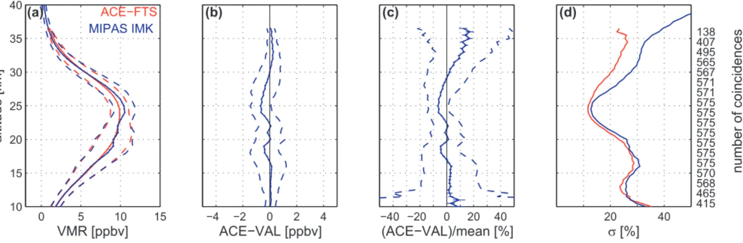
0 5 10 15 10 15 20 25 30 35 40 ACE−FTS MIPAS IMK (a) VMR [ppbv] altitude [km] −4 −2 0 2 4 ACE−VAL [ppbv] (b) −40 −20 0 20 40 (c) (ACE−VAL)/mean [%] 20 40 (d) σ [%] 415 465 568 570 575 575 575 575 575 575 575 571 571 567 565 495 407 138 number of coincidences
Fig. 7. Same as Fig. 2 but for HNO
3comparison between ACE-FTS and the MIPAS IMK-IAA data product for coincident measurements
between 30
◦N–90
◦N(±9 h, 800 km, ±3×10
−6K m
2kg
−1s
−1at 475 K).
Fig. 7. Same as Fig. 2 but for HNO3comparison between ACE-FTS and the MIPAS IMK-IAA data product for coincident measurements
between 30◦N–90◦N (±9 h, 800 km, ±3×10⁻⁶K m2kg−1s−1at 475 K).
papers as ±9 h, 800 km, and a maximum potential vorticity (PV) difference of ±3×10⁻⁶K m2kg−1s−1at 475 K poten-tial temperature. Wang et al. (2007a) and Wang et al. (2007b) compared about 600 daytime and nighttime MIPAS profiles to about 350 ACE-FTS coincident profiles, separated into two different latitude bands: 30–60◦and 60–90◦, resulting in a mean distance of 280±151 km and a mean time difference of 7.1±8.4 h. The consistency between both MIPAS HNO3 products (ESA and IMK-IAA) and ACE-FTS HNO3 was found to be very good. The mean differences were between ±0.1 and −0.5 ppbv for the ACE-FTS versus MIPAS ESA data product comparisons (Wang et al., 2007a) and between ±0.1 and −0.7 ppbv for the ACE-FTS versus MIPAS IMK-IAA data product comparisons (Wang et al., 2007b). That corresponds to relative differences between ±5 and ±10% for altitudes between 10 and 30 km and between ±10 and ±15% for altitudes above (up to 35 km) (Wang et al., 2007a,b).
In both papers, data were analysed for the period 9 Febru-ary to 25 March 2004, including data from the ACE satel-lite commissioning period which continued until 21 February 2004. We recalculated the comparisons between ACE-FTS sunset observations and MIPAS for the period 21 February to 25 March 2004 using only data from the ACE Science Operations period. Figures 6 and 7 show the results of these revised comparisons.
For the comparison with the MIPAS ESA data used in this work (v4.62), we narrowed the coincidence criteria to ±6 h and 300 km, resulting in 138 coincident profiles, shown in Fig. 6. The mean difference between ACE-FTS and MI-PAS ESA HNO3is typically −0.1 ppbv and varies between
−0.71 ppbv at 27.5 km and +0.33 ppbv at 30.5 km. That cor-responds to typically ±2% between 10 and 27 km and to ±9% between 27 and 36 km. A maximum relative difference of −25% is obtained for the highest comparison altitude of 36.5 km.
3542 M. A. Wolff et al.: Validation of HNO3, ClONO2and N2O5from ACE-FTS 0 0.5 1 1.5 2 10 15 20 25 30 35 40 ACE−FTS MIPAS IMK (a) VMR [ppbv] altitude [km] −0.3 −0.1 0 0.1 0.3 ACE−VAL [ppbv] (b) −40 −20 0 20 40 (c) (ACE−VAL)/mean [%] 0 20 40 60 80 100 (d) σ [%] 559 570 578 578 580 580 580 580 580 576 576 564 460 261 151 number of coincidences 0 0.5 1 1.5 2 10 15 20 25 30 35 40 ACE−FTS MIPAS IMK CTM (a) VMR [ppbv] altitude [km] −0.3 −0.1 0 0.1 0.3 ACE−VAL [ppbv] (b) −40 −20 0 20 40 (c) (ACE−VAL)/mean [%] 0 20 40 60 80 100 (d) σ [%] 559 570 578 578 580 580 580 580 580 576 576 564 460 261 151 number of coincidences
Fig. 8. Same as Fig. 2 but for ClONO
2comparisons between ACE-FTS and the MIPAS IMK-IAA data product for coincident measurements
between 30
◦N–90
◦N (±9 h, 800 km, ±3×10
−6K m
2kg
−1s
−1at 475 K ). Panels (c) also show the mean relative deviation from the mean,
calculated using Eq. (4) (cyan solid line) with ±1σ relative standard deviation (cyan dashed line). Top row: MIPAS uncorrected data. Bottom
row: MIPAS CTM-corrected data.
Fig. 8. Same as Fig. 2 but for ClONO2comparisons between ACE-FTS and the MIPAS IMK-IAA data product for coincident measurements
between 30◦N–90◦N (±9 h, 800 km, ±3×10⁻⁶K m2kg−1s−1at 475 K ). Panels (c) also show the mean relative deviation from the mean, calculated using Eq. (4) (cyan solid line) with ±1σ relative standard deviation (cyan dashed line). Top row: MIPAS uncorrected data. Bottom row: MIPAS CTM-corrected data.
The comparison between the ACE-FTS and MIPAS (IMK-IAA v8) HNO3products was calculated using the same co-incidence criteria as defined by Wang et al. (2007b) and is shown in Fig. 7. Between 10 and 31 km, ACE-FTS is typi-cally 0.2 ppbv smaller than MIPAS IMK-IAA HNO3. Mean relative differences are mainly within ±2% and do not exceed ±9%. Above 31 km, ACE-FTS reports larger values than MI-PAS. The mean relative differences are between 5 and 17%. 4.3.2 ClONO2
MIPAS ClONO2VMR data are retrieved with the IMK-IAA scientific data processor using the microwindow centered at 780.2 cm−1. H¨opfner et al. (2007) compared ClONO2 profiles from MIPAS (IMK-IAA v10/11) with ACE-FTS ClONO2 profiles for the period 9 February to 25 March 2004. Comparisons were carried out for the latitude bands 30–60◦N and 60–90◦N and separated for MIPAS daytime and nighttime measurements. Coincidence criteria used for the ClONO2 comparisons were ±9 h, 800 km, and a
maxi-mum PV difference of ±3×10⁻⁶K m2kg−1s−1at 475 K po-tential temperature. When combining all coincidences, the mean differences between ACE-FTS and MIPAS ClONO2 were found to be less than 0.04 ppbv (<5%) up to altitudes of 27 km. At nearly all altitudes, ACE-FTS reported smaller VMR values than MIPAS. Above 27 km, the differences in-creased to around −0.15 ppbv (−30% at 34.5 km). In the altitude range between 15 and 19 km, slightly enhanced dif-ferences of up to −0.03 ppbv could be observed (H¨opfner et al., 2007). The high-altitude bias was assumed to be pho-tochemically induced. Therefore, H¨opfner et al. (2007) used the KArlsruhe SImulation model of the Middle Atmosphere Chemical Transport Model (KASIMA CTM) (Kouker et al., 1999) to transform the MIPAS profiles to the time and loca-tion of ACE-FTS occultaloca-tions. From a multi-annual run with a horizontal resolution of approximately 2.6×2.6◦ (T42), a vertical resolution of 0.75 km from 7 to 22 km and an ex-ponential increase above with a resolution of about 2 km in the upper stratosphere, and a model time step of 6 min, ClONO2profiles were interpolated to the time and position
M. A. Wolff et al.: Validation of HNO3, ClONO2and N2O5from ACE-FTS 3543 of the measurements of ACE-FTS and of MIPAS: xCTMACE and
xCTMMIPAS. For the intercomparison, the original MIPAS pro-files xMIPASwere transformed to the time and position of the ACE-FTS measurements by adding the relative difference between the two model results. Relative differences were used to account for any problems with the absolute values of modeled NOy. The expression used is:
xCTMcorrMIPAS =xMIPAS+
xCTMACE −xCTMMIPAS xCTMMIPAS
×xMIPAS. (5)
In the resulting comparison between ACE-FTS and the CTM-corrected MIPAS ClONO2 VMRs, the maximum ab-solute differences were reduced and no systematic bias up to 27 km altitude was seen. At higher altitudes, however, the model overcompensated for the photochemically-induced bias and the corrected MIPAS ClONO2 values were up to 0.1 ppbv smaller than those measured by ACE-FTS (H¨opfner et al., 2007).
For this paper, we recalculated the comparison between ACE-FTS and MIPAS ClONO2using IMK-IAA v11 for the period 21 February to 25 March 2004, considering only the ACE-FTS data after the start of the ACE Science Opera-tions period. The results of the comparisons, which do not change significantly the findings of H¨opfner et al. (2007), are shown in Fig. 8. The ACE-FTS ClONO2values are smaller than the uncorrected MIPAS product for all altitudes. The mean relative differences are better than −7% between 16 and 27 km, and reach −30% at 34 km (Fig. 8, top row). The comparison between ACE-FTS and the CTM-corrected MI-PAS ClONO2 profiles shows no systematic difference be-tween 16 and 27 km. Typically mean relative differences are within ±1%, reaching a maximum of −6% around 16– 17 km. Above 27 km, ACE-FTS ClONO2is larger than the corrected MIPAS values with a maximum relative difference of 22% around 33 km (Fig. 8, bottom row), suggesting that the model is overcompensating as observed in the previous study.
As explained in Sect. 3, Eq. (3) overestimates the rela-tive differences in the lowest altitude region, 13–16 km, when some denominators are extremely small. Therefore, profiles of the relative deviation of the mean, calculated with Eq. (4), are also included in Fig 8. The relative deviation of the mean clearly shows that ACE-FTS is very consistent with MIPAS ClONO2also at lower altitudes, differing not more than −6% between 13 and 16 km.
4.3.3 N2O5
The retrieval method and characteristics of N2O5 profiles inverted from MIPAS observations have been described by Mengistu Tsidu et al. (2004). N2O5is retrieved from its in-frared emission in the ν12 band in the spectral range from 1239–1243 cm−1. Spectroscopic data for N2O5by Wagner and Birk (2003) were taken from the HITRAN 2004 database
(Rothman et al., 2005). The vertical resolution, in the case of mid-latitude profiles, is about 4–6 km between 30 and 40 km and 6–8 km below 30 km and between 40 and 50 km. The measurement noise is between 5 and 30% in the altitude range of 20–40 km. The systematic errors are within 10–45% at 20–40 km and increase up to 75% outside this region.
Here we compare N2O5 profiles from ACE-FTS ob-servations and MIPAS IMK-IAA v9 measurements from 21 February 2004 until 25 March 2004. For the comparisons, we again used as coincidence criteria a maximum time differ-ence of ±9 h, a maximum tangent point differdiffer-ence of 800 km, and a maximum PV difference of ±3×10⁻⁶km2kg−1s−1at the 475 K potential temperature level.
In Fig. 9, we show separately the results of the com-parisons between ACE-FTS and MIPAS IMK-IAA daytime (first row) and MIPAS IMK-IAA nighttime N2O5 profiles (third row). To account for the differing vertical resolution between MIPAS and ACE-FTS in the lower stratosphere, we convolved the ACE-FTS N2O5profiles with the MIPAS av-eraging kernels and included this additional comparison in Fig. 9. MIPAS measurements occur either in the late morn-ing or early night, while the ACE-FTS observations used here are made during sunset. Thus, for comparison with night-time MIPAS observations, the night-time difference (ACE-FTS– MIPAS) is −4 to −5 h, while in the case of MIPAS daytime measurements it is about +6 to +8 h.
At the altitude of the N2O5 VMR maximum (around 30 km), ACE-FTS VMRs are ∼0.5 ppbv (75%) smaller than MIPAS IMK-IAA daytime observations and ∼0.4 ppbv (70%) smaller than the MIPAS IMK-IAA nighttime obser-vations. At altitudes below the VMR maximum, these differ-ences decrease in absolute terms.
In relative terms, the largest differences appear at around 18 km and at the highest altitudes, just below 40 km. The differences at lower altitudes are partly due to the differ-ences in vertical resolution between MIPAS and ACE-FTS there. These are strongly reduced to 20–30% for MIPAS daytime comparisons and 50% for MIPAS nighttime com-parisons when MIPAS averaging kernels are taken into ac-count.
To account for the diurnal cycle of N2O5and the different local observation times of MIPAS and ACE-FTS, we have performed a correction using the KASIMA CTM (Kouker et al., 1999), as was done for ClONO2. Rows 2 and 4 of Fig. 9 show results of the CTM-corrected comparisons for MIPAS IMK-IAA daytime and MIPAS IMK-IAA nighttime measurements, respectively. In both cases, the large differ-ences at the VMR maximum are reduced by a factor of 2–4 and the difference profiles for daytime and nighttime com-parisons have become more similar. In relative units, ACE-FTS N2O5is now about ∼40% smaller than MIPAS IMK-IAA near the VMR maximum. At lower altitudes, the max-imum differences are further reduced when comparing the convolved ACE-FTS VMRs with the MIPAS IMK-IAA day-and nighttime measurements.
3544 M. A. Wolff et al.: Validation of HNO3, ClONO2and N2O5from ACE-FTS 0 0.5 1 1.5 10 15 20 25 30 35 40 ACE−FTS ACE−FTS sm MIPAS IMK day
(a) VMR [ppbv] altitude [km] −0.5−0.25 0 0.25 0.5 ACE−VAL [ppbv] (b) −200 −100 0 100 200 (c) (ACE−VAL)/mean [%] 50 100 150 200 (d) σ [%] 118 216 259 266 274 275 275 275 273 273 271 270 270 250 206 108 59 number of coincidences 0 0.5 1 1.5 10 15 20 25 30 35 40 ACE−FTS ACE−FTS sm MIPAS IMK d CTM (a) VMR [ppbv] altitude [km] −0.5−0.25 0 0.25 0.5 ACE−VAL [ppbv] (b) −200 −100 0 100 200 (c) (ACE−VAL)/mean [%] 50 100 150 200 (d) σ [%] 118 216 259 266 274 275 275 275 273 273 271 270 270 250 206 108 59 number of coincidences
Fig. 9. Same as Fig. 2 but for N2O5 comparisons between ACE-FTS and MIPAS IMK-IAA data product for coincident measurements
between 30◦N–90◦N (±9 h, 800 km, ±3×10⁻⁶K m2kg−1s−1at 475 K ). The orange lines show the comparisons between smoothed (sm)
ACE-FTS and MIPAS IMK-IAA data product for the same coincidences. Panels (c) also show the mean relative deviation from the mean, calculated using Eq. (4) (cyan solid line) with ±1σ relative standard deviation (cyan dashed line). First row: MIPAS daytime measurements; second row: CTM-corrected MIPAS daytime measurements; third row: MIPAS nighttime measurements; fourth row: CTM-corrected MIPAS nighttime measurements.
M. A. Wolff et al.: Validation of HNO
3, ClONO
2and N
2O
5from ACE-FTS
39
0 0.5 1 1.5 10 15 20 25 30 35 40 ACE−FTS ACE−FTS sm MIPAS IMK night
(a) VMR [ppbv] altitude [km] −0.5−0.25 0 0.25 0.5 ACE−VAL [ppbv] (b) −200 −100 0 100 200 (c) (ACE−VAL)/mean [%] 50 100 150 200 (d) σ [%] 120 220 289 296 297 299 299 299 297 297 297 296 296 268 212 105 54 number of coincidences 0 0.5 1 1.5 10 15 20 25 30 35 40 ACE−FTS ACE−FTS sm MIPAS IMK n CTM (a) VMR [ppbv] altitude [km] −0.5−0.25 0 0.25 0.5 ACE−VAL [ppbv] (b) −200 −100 0 100 200 (c) (ACE−VAL)/mean [%] 50 100 150 200 (d) σ [%] 120 220 289 296 297 299 299 299 297 297 297 296 296 268 212 105 54 number of coincidences
Fig. 9. Continued.Fig. 9. Same as Fig. 2 but for N2O5comparisons between ACE-FTS and MIPAS IMK-IAA data product for coincident measurements
between 30◦N–90◦N (±9 h, 800 km, ±3×10⁻⁶K m2kg−1s−1at 475 K ). The orange lines show the comparisons between smoothed (sm) ACE-FTS and MIPAS IMK-IAA data product for the same coincidences. Panels (c) also show the mean relative deviation from the mean, calculated using Eq. (4) (cyan solid line) with ±1σ relative standard deviation (cyan dashed line). First row: MIPAS daytime measurements; second row: CTM-corrected MIPAS daytime measurements; third row: MIPAS nighttime measurements; fourth row: CTM-corrected MIPAS nighttime measurements.