HAL Id: hal-00295186
https://hal.archives-ouvertes.fr/hal-00295186
Submitted on 19 Apr 2002
HAL is a multi-disciplinary open access
archive for the deposit and dissemination of
sci-entific research documents, whether they are
pub-lished or not. The documents may come from
teaching and research institutions in France or
abroad, or from public or private research centers.
L’archive ouverte pluridisciplinaire HAL, est
destinée au dépôt et à la diffusion de documents
scientifiques de niveau recherche, publiés ou non,
émanant des établissements d’enseignement et de
recherche français ou étrangers, des laboratoires
publics ou privés.
model and retrieved data from GOME measurements
A. Lauer, M. Dameris, A. Richter, J. P. Burrows
To cite this version:
A. Lauer, M. Dameris, A. Richter, J. P. Burrows. Tropospheric NO2 columns: a comparison between
model and retrieved data from GOME measurements. Atmospheric Chemistry and Physics, European
Geosciences Union, 2002, 2 (1), pp.67-78. �hal-00295186�
www.atmos-chem-phys.org/acp/2/67/
Atmospheric
Chemistry
and Physics
Tropospheric NO
2
columns: a comparison between model and
retrieved data from GOME measurements
A. Lauer1, M. Dameris1, A. Richter2, and J. P. Burrows2
1DLR Institut f¨ur Physik der Atmosph¨are, Oberpfaffenhofen, D-82234 Wessling, Germany 2Institut f¨ur Umweltphysik, Universit¨at Bremen, D-28359 Bremen, Germany
Received: 31 October 2001 – Published in Atmos. Chem. Phys. Discuss.: 13 December 2001 Revised: 3 April 2002 – Accepted: 12 April 2002 – Published: 19 April 2002
Abstract. Tropospheric NO2 plays a variety of significant
roles in atmospheric chemistry. In the troposphere it is one of the most significant precursors of photochemical ozone (O3) production and nitric acid (HNO3). In this study
tro-pospheric NO2 columns were calculated by the fully
cou-pled chemistry-climate model ECHAM4.L39(DLR)/CHEM. These have been compared with tropospheric NO2columns,
retrieved using the tropospheric excess method from mea-surements by the Global Ozone Monitoring Experiment (GOME) of up-welling earthshine radiance and the extrater-restrial irradiance. GOME is part of the core payload of the second European Research Satellite (ERS-2). For this study the first five years of GOME measurements have been used. The period of five years of observational data is sufficiently long to facilitate for the first time a comparison based on cli-matological averages with global coverage, focussing on the geographical distribution of the tropospheric NO2.
A new approach of analysing regional differences (i.e. on continental scales) by calculating individual averages for different environments provides more detailed information about specific NOxsources and of their seasonal variations.
The results obtained enable the validity of the model NO2
source distribution and the assumptions used to separate tro-pospheric and stratospheric parts of the NO2column amount
from the satellite measurements to be investigated.
1 Introduction
Tropospheric NO2plays a key role in both stratospheric and
tropospheric chemistry. In the troposphere the photolysis of NO2 results in the formation of O3 (e.g. Bradshaw et
al., 2000). NO2 can then be regenerated by catalytic
cy-cles involving both organic peroxy radicals (RO2), the
hydro-peroxyradical (HO2), the hydroxyl radical (OH) and volatile
Correspondence to: A. Lauer ([email protected])
organic compounds (VOC) and carbon monoxide (CO). In addition, NO2 can react with O3to form the nitrate radical
(NO3), which is a strong oxidant and plays an important role,
particularly in NOx polluted areas at night (Wayne, 1991).
Thus NO2is one of the key species in determining the
oxi-dising capacity of the troposphere. For more details on the role of NO2in atmospheric chemistry, the reader is referred
to Finlayson-Pitts and Pitts (1999).
Although direct absorption of ultraviolet and visible radia-tion by tropospheric NO2is not thought to provide a large
at-mospheric forcing, local maxima of up to 0.1 to 0.15 Wm−2 can be reached (Velders et al., 2001). As tropospheric O3is
also a significant greenhouse gas, NO2also contributes
indi-rectly to radiative forcing.
The emission of NOx(NOx=NO + NO2) into the
tropo-sphere is strongly influenced by human activities, NOx
be-ing produced in significant amounts by industrial combus-tion and biomass burning (Lee et al., 1997). Natural sources of NOxare lightning and emissions from soils in the
tropo-sphere. For further details on the contributions to the global NOxbudget, see e.g. Brasseur et al. (1999). NO2is known
to impact on human health and the environment both directly and through the production of O3(e.g. EPA, 2000). Overall
it is necessary to monitor and understand the global impact of this pollutant on the physics and chemistry of the atmo-sphere.
The launch of GOME aboard the ERS-2 in April 1995 has enabled the global observation of the distribution of NO2,
which has significant amounts in both the stratosphere and the troposphere (Burrows et al., 1999). Further the develop-ment of the tropospheric excess method has enabled tropo-spheric NO2columns to be retrieved on scales up to global
for the first time (Burrows et al., 1999), (Richter and Bur-rows, 2001). This retrieved data product provides a set of long-term observational data, which are well suited for eval-uating the quality of the results of chemistry-climate models. In this study, in contrast to recent studies by Leue et
al. (2001) and Velders et al. (2001), climatological aver-ages of the tropospheric NO2columns retrieved from GOME
have been used. These have been compared with those obtained from the interactively coupled chemistry-climate model ECHAM4.L39(DLR)/CHEM on global and regional scales. Monthly average values of the NO2 tropospheric
columns retrieved using the TEM algorithm (“Tropospheric Excess Method”) from five years of GOME observations (January 1996 to August 2000) and 20 years of model output provide the data base.
This comparison of modelled and measured tropospheric NO2column amounts is the first step in evaluating the
abil-ity of ECHAM4.L39(DLR)/CHEM to simulate the tropo-spheric NOx chemistry and to unveil still present
deficien-cies in chemistry and emission datasets. This first step is necessary to prepare future studies on the global impact of traffic (road and aircraft) induced NOx emissions on
cli-mate and air chemistry as well as their contribution to the global NOx budget in comparison to other man-made
(in-dustry and biomass burning) and natural (soils and light-ning) NOx emissions. Once the chemistry-climate model
ECHAM4.L39(DLR)/CHEM has been adjusted and evalu-ated to reproduce present and past global NOx
measure-ments, prognostic simulations of future scenarios will be un-dertaken.
To achieve optimum comparability of the two different data sources, the satellite data have been fitted to the lower resolution of the model grid. The tropospheric NO2columns
from the model data have been calculated in two ways: 1. Integration from the surface up to the (thermal) model
tropopause (“Thermal Tropopause”-method).
2. Separation of tropospheric and stratospheric NO2
amount using the method applied to the satellite data (“Tropospheric Excess or Reference Sector Method”).
2 Data
2.1 Tropospheric NO2 columns retrieved from GOME
observations
GOME is a spectrometer on board ERS-2, which was launched on 20 April 1995 and flies in a sun-synchronous, polar orbit at an average height of 785 km above the Earth’s surface (Burrows et al., 1999, and references therein). The GOME instrument observes in nadir viewing geometry the light (UV/visible) scattered back from the atmosphere and reflected at the ground. Once per day, it also observes the ex-traterrestrial solar irradiance. The instrument is designed to observe simultaneously the spectral range between 232 and 793 nm. The atmosphere is scanned with a spatial resolution of 320 km × 40 km (across track × along track) (forward scan) and 960 km × 40 km (back scan). Each individual orbit
of ERS-2 takes about 100 min. Although the repeating cy-cle of an orbit is 35 days, nearly global coverage (except for a small gap around the poles) is achieved within three days applying the maximum scan width of 960 km (ESA, 1995). As a result of the sun-synchronous orbit, the measurements in low and middle latitudes are always taken at the same lo-cal time (LT) (the northern mid-latitudes are crossed at about 10:45 LT).
The trace gas retrieval of NO2is achieved using the DOAS
technique (Differential Optical Absorption Spectroscopy). This technique utilizes the atmospheric absorption, defined as the natural logarithm of the ratio of the extraterrestrial ir-radiance and the earthshine ir-radiance, for a selected spectral window. This is compared with reference absorption spectra of gases absorbing in the spectral window and a polynomial of low order. The polynomial describes the scattering and broad absorption in the window. The slant column of a gas is derived from the differential absorption of the gas in ques-tion and in first approximaques-tion is the integrated concentraques-tion along the light paths through the atmosphere. For this study, the spectral window from 425 to 450 nm has been used, the spectra of NO2, O3, O4and H2O and a reference Ring
spec-trum being fitted (Richter and Burrows, 2001).
The resultant slant columns of NO2 can be converted to
vertical columns by the application of an air mass factor, AMF. The AMF describes the effective length of the light path through the atmosphere and is derived from radiative transfer calculations. The value of the AMF depends on the viewing geometry and the solar zenith angle, but also on surface albedo, vertical gas profile, clouds and atmospheric aerosol. In this study, a constant vertical profile with all NO2 in a 1.5 km boundary layer has been assumed.
Strato-spheric NO2 is not included in the airmass factor
calcula-tion as the tropospheric slant columns have already been cor-rected for the stratospheric contribution, and the influence of stratospheric NO2 on the radiative transfer can be
ne-glected. (Richter and Burrows, 2001; Velders et al., 2001). A brief summary of the assumptions for derivation of the tro-pospheric NO2 column amounts from the GOME
measure-ments is given by Table 1.
The uncertainties introduced by the most relevant assump-tions are discussed in Sect. 4.2. Details and a full error anal-ysis can be found in Richter and Burrows (2001).
The Tropospheric Excess or Reference Sector Method for determining the tropospheric columns of NO2makes two
as-sumptions:
a) the longitudinal distribution of stratospheric NO2is
rel-atively homogeneous. This is reasonable at latitudes be-low 60◦N through the year, because the bulk of the NO2
in the stratosphere is at a relatively high altitude and as a result determined by photolysis and therefore mainly by day length which is a function of latitude only. b) at remote locations over the Pacific, the tropospheric
negligi-Table 1. Summary of the assumptions for derivation of the tropospheric NO2column amounts from the GOME measurements (version 1.0
of the IUP/IFE-UB TEM NO2Dataset) (after Richter and Burrows, 2001). Negative values indicate error sources that tend to lead to an
underestimation of the tropospheric NO2
Assumption Purpose Uncertainty
longitudinal homogeneity of the stratospheric NO2column amounts separation of tropospheric and
strato-spheric amount (TEM)
<1 × 10¹⁵molec/cm2 constant and negligibly small tropospheric NO2 column amounts in
the reference sector above the Pacific at longitude 170◦W to 180◦W
separation of tropospheric and strato-spheric amount (TEM)
<5 × 10¹⁴molec/cm2 constant vertical profile with all NO2in a 1.5 km boundary layer tropospheric AMF calculation ±50%
clear sky conditions tropospheric AMF calculation −30%
surface albedo of 0.05 tropospheric AMF calculation ±50%
NO2absorption cross-section for stratospheric temperatures (241 K) NO2fit (DOAS) −20%
Table 2. Nitrogen Oxide emissions as used in the E39/C model simulation (Hein et al., 2001) and the range of uncertainty (Bradshaw et al., 2000)
Source Emissions [Tg(N)/yr] Range [Tg(N)/yr] Contribution [%] Reference
Industry 22.6 16–30 57.8 Benkovitz et al. (1996)
Soils 5.5 3–8 14.1 Yienger and Levy (1995)
Lightning 5.4 ± 0.1 (clim. annual mean) 3.2–261 13.8 Price and Rind (1992)
Biomassburning 5.0 4–16 12.8 Hao et al. (1990)
Aircraft 0.6 0.5–0.6 1.5 Schmitt and Brunner (1997)
Total 39.1 26.7–80.6 100.0
1free troposphere + near surface
bly small. This is shown by the results of aircraft surements (Schultz et al., 1999) and by the GOME mea-surements themselves (Richter and Burrows, 2001). Thus the TEM tropospheric columns of NO2are determined
by subtracting the NO2column at a selected remote and clean
location from that at other locations at the same latitude. In this study the reference clean sector is chosen to be around the international date line at longitude 180◦W.
For this study, climatological monthly means of the tropo-spheric NO2column amounts (January 1996 to August 2000)
have been used. The data were selected to be cloud free, i.e. only pixels having a cloud coverage below a threshold value 10% were used to derive the tropospheric NO2column
amounts from the GOME measurements (see also Sect. 4.2). (Version 1.0 of the IUP/IFE-UB TEM NO2Dataset.)
2.2 ECHAM4.L39(DLR)/CHEM
ECHAM4.L39(DLR)/CHEM (hereafter referred to as E39/C) is a spectral atmospheric chemistry – general circulation model. The model consists of two parts, the atmosphere general circulation model ECHAM4.L39(DLR) (Land et al., 1999) and the chemistry module CHEM
(Steil et al., 1998). ECHAM4.L39(DLR) and CHEM are fully coupled, facilitating the representation of feedback mechanisms between changes in concentrations of chemical species and the simulated dynamics. E39/C has a horizontal resolution of T30 (3.75◦×3.75◦) and 39 layers in the vertical direction extending from the surface up to 10 hPa (30 km). The chemistry module CHEM includes 107 reactions and 37 trace gases in the troposphere and stratosphere. It is connected with the ECHAM4 radiation scheme via H2O, O3,
CH4, N2O and CFCs. The system thereby allows feedbacks
between chemistry and the radiation scheme, which in turn, affects dynamics.
The current chemical scheme within CHEM does not in-clude the NOxreservoir species PAN. In addition, CHEM
neither includes VOC chemistry nor the heterogeneous re-action of N2O5 on the surface of wet aerosols in the
tro-posphere forming HNO3. This version of E39/C is
special-ized on stratospheric ozone chemistry. Nevertheless, this first look not only provides a detailed view into the current ability and deficiencies of E39/C to simulate tropospheric NOx, but
also enables the validation of the seasonal variation of cur-rently used NOx emission data sets, as e.g. biomass
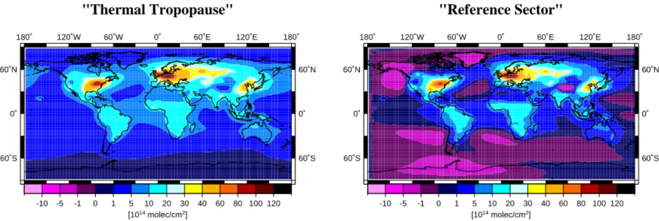
180˚ 120˚W 60˚W 0˚ 60˚E 120˚E 180˚ 60˚S 60˚S 0˚ 0˚ 60˚N 60˚N "Thermal Tropopause" -10 -5 -1 0 1 5 10 20 30 40 60 80 100 120 [1014 molec/cm2] 180˚ 120˚W 60˚W 0˚ 60˚E 120˚E 180˚ 60˚S 60˚S 0˚ 0˚ 60˚N 60˚N "Reference Sector" -10 -5 -1 0 1 5 10 20 30 40 60 80 100 120 [1014 molec/cm2]
Fig. 1. E39/C, climatological annual means based on 20 years of the modelled tropospheric NO2column amounts, showing the results of
the two different methods of calculation.
the present, past and future global impact of man-made NOx
emissions (especially road-traffic and aircraft) in comparison to the natural (soils and lightning) NOx emissions not only
on the climate (e.g. tropospheric O3production) but also on
air chemistry (e.g. OH budget) and air quality.
Possible effects of the limitations on tropospheric NOx
chemistry are discussed in Sect. 4.1.
For this study an existing dataset from the “1990” control experiment (Hein et al., 2001) has been used. The E39/C data used for this comparison represent the beginning of the 1990s. Therefore the model was run in quasi-equilibrium mode. Gas emissions, Sea Surface Temperature (SST), and boundary conditions were assumed similar to those measured or determined for the year 1990. A detailed model descrip-tion and model applicadescrip-tions can be found in Hein et al. (2001) and Schnadt et al. (2001).
Table 2 summarizes the Nitrogen Oxide emissions as con-sidered for this model simulation. The total sum equals 39.1 Tg(N)/yr. The emissions from industry and ground based traffic, which are predominantly emitted by the east-ern United States, Central Europe and Japan, have the major contribution of about 58% of the global budget. (This dataset is based on version 1A of the GEIA global inventories of the annual emissions of NOxfrom anthropogenic sources around
the year 1985, Benkovitz et al., 1996). Especially in the trop-ics, biomass burning and lightning are the most important NOx sources. In addition emissions from soils and aircraft
are explicitly taken into account.
3 Model data analyses and comparisons
In this study two methods have been used to calculate the tropospheric NO2 columns from the model data. The first
approach is to integrate the NO2concentration from the
sur-face to the tropopause which is determined by employing the thermal WMO-criterion. This dataset is defined as the “Ther-mal Tropopause” dataset.
The second approach applies the TEM to the model data in a manner similar to that applied to the GOME observations. The averaged total column over a Pacific sector (170◦W to 180◦W) as estimate for the stratospheric amount (Richter and Burrows, 2001). The tropospheric column is calcu-lated by subtracting this approximation of the stratospheric amount from the total columns.
The model results have been compared to each other. Al-though the “TEM” dataset yields smaller absolute values, the qualitative seasonal variation is not affected in any of the cases studied. Figure 1 shows the results of the two methods of calculation applied to the model output of E39/C. To calculate the climatological annual means, all 20 model years are used. As it can be seen easily, all major features of the global pattern are conserved. In both cases, the areas with high NOxemissions (namely United States, Central
Eu-rope and Southeast Asia/Japan) are clearly visible. Even the distribution of the patterns of regions with lower values of the tropospheric NO2 column amounts (e.g. Africa, South
America, Australia) are (in a qualitative sense) similar. Comparison of the two different methods of calculation indicates that:
1. For the “Thermal Tropopause” dataset, the regions with high values of the tropospheric NO2 column amounts
have a somewhat larger extent and higher maximum val-ues than the results of “TEM”.
2. For the “TEM” dataset, negative values become possi-ble in regions with low NO2column amounts, e.g. over
the oceans.
3. In regions with very low tropospheric NO2 column
amounts (e.g. the oceans) “TEM” has a large inherent error resulting from subtraction of two similar quanti-ties.
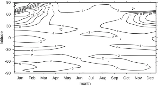
-90 -60 -30 0 30 60 90 latitude month
Jan Feb Mar Apr May Jun Jul Aug Sep Oct Nov Dec
0 0 0 2 2 2 2 2 2 2 2 2 2 2 4 4 4 4 4 4 4 4 4 6 6 6 8 8 10 10 12
Fig. 2. Seasonal variation of the averaged climatological tropospheric NO2column amounts (1014molec/cm2) for the reference sector over
the Pacific Ocean (170◦W to 180◦W) as modelled by E39/C (“Thermal Tropopause”-method). In contrast, “TEM” assumes no tropospheric NO2being present in the reference sector.
4. The results over the continents are quite reasonable: the annual mean relative difference of both methods being below 30% for most of the examined regions.
The reason for the lower values obtained by TEM with model data is that significant concentrations of NO2are
gen-erated by the model at 170◦W to 180◦W. This appears to be outflow from the continents which is predominantly the case in the northern mid-latitudes in winter and results in a background of (1 to 7) ×1014molec/cm2north of 60◦S and
< 1 × 10¹⁴molec/cm2 south of 60◦S. In the remote mar-itime boundary layer assuming the height of the PBL to be 2 km this would correspond to 20 to 150 pptv. This may indi-cate that in the model the NO2is not being removed rapidly
enough.
When looking at the model data one must keep in mind that the model domain does not extend above 10 hPa. Thus the stratospheric amounts calculated by the model do neither include NO2in the upper stratosphere nor in the mesosphere.
This could reduce the total variability of the stratospheric columns by up to 1/3 and might also explain some of the variability over Antarctica, as seen in the TEM model data.
However, as mentioned before, the seasonal variation of the studied regions is not affected by “TEM”, because (especially in the northern mid-latitudes in winter) the tropo-spheric NO2 column amounts are several times higher than
the overestimation of stratospheric NO2by the NO2 above
the reference sector. Figure 2 shows the averaged tropo-spheric NO2column amounts as modelled by E39/C above
the reference sector over the Pacific Ocean.
3.1 Global comparison
For optimal comparison between the model results and the TEM dataset derived from GOME, in the following only model results obtained using TEM are compared to the GOME data (Fig. 3).
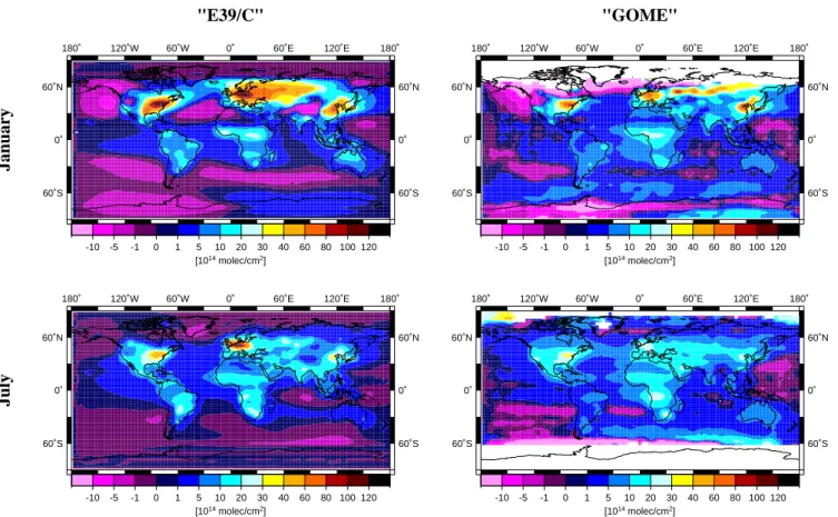
In January, both the satellite and the model data clearly show the large northern hemispheric NOx emission areas.
These are caused by anthropogenic emissions from domes-tic heating, industry and road traffic: USA (pardomes-ticularly the eastern part), Europe and Southeast Asia/Japan. These areas can be easily identified by the high values of the tropospheric NO2column amounts.
A significant difference can be seen between the model-and satellite data in these regions: E39/C produces larger maxima and the regions of enhanced tropospheric NO2
col-umn amounts have a larger spatial extent than those observed in the satellite data.
On the other hand, the high NO2areas in central and
south-ern Africa (caused by biomass burning and lightning pro-duced NOx) of both data sources are in good agreement: the
location and the absolute column amounts being similar. In January the GOME data show much higher variation of the NO2 amounts over Antarctica than the model data
(Fig. 3). Although the GOME data for Antarctica must be treated very carefully as not all assumptions made for the tro-pospheric NO2retrieval from the GOME measurements (see
Table 1 and Sect. 4.2) are valid for this region, this might indicate widespread NOxemissions by sunlight from snow.
The production of NO2in or just above snow is believed to
result from the photolysis of HNO3carried to the Antarctic in
the snow (e.g. Jones et al., 2001). This cycling mechanism is certainly not in the model yet, but the differential signal may be seen by GOME. The signal could be positive or negative
180˚ 120˚W 60˚W 0˚ 60˚E 120˚E 180˚ 60˚S 60˚S 0˚ 0˚ 60˚N 60˚N "E39/C" -10 -5 -1 0 1 5 10 20 30 40 60 80 100 120 [1014 molec/cm2] January 180˚ 120˚W 60˚W 0˚ 60˚E 120˚E 180˚ 60˚S 60˚S 0˚ 0˚ 60˚N 60˚N "GOME" -10 -5 -1 0 1 5 10 20 30 40 60 80 100 120 [1014 molec/cm2] 180˚ 120˚W 60˚W 0˚ 60˚E 120˚E 180˚ 60˚S 60˚S 0˚ 0˚ 60˚N 60˚N -10 -5 -1 0 1 5 10 20 30 40 60 80 100 120 [1014 molec/cm2] July 180˚ 120˚W 60˚W 0˚ 60˚E 120˚E 180˚ 60˚S 60˚S 0˚ 0˚ 60˚N 60˚N -10 -5 -1 0 1 5 10 20 30 40 60 80 100 120 [1014 molec/cm2]
Fig. 3. Climatological monthly means of the tropospheric column amounts calculated by E39/C (‘TEM’) and derived from GOME measure-ments for January and July, respectively. Blank (white coloured) areas are data gaps.
in the TEM dataset, because it depends whether the region selected for the reference sector is producing some NO2by
this mechanism or not. In addition, tropospheric NOxhas a
longer lifetime under these colder and probably low O3
con-ditions. However, it has to be emphasized this is still very speculative at this stage.
In July, the tropospheric NO2column amounts reflect the
reduction in the NOxemission in North America, Europe and
Asia: both the magnitude of the NO2 clouds and their
ar-eas being reduced in size in comparison to those of January. Again, these areas have a larger extent and higher maxima in the model data than shown by the GOME data.
These observations are in general consistent with the observation that relatively high NO2 values are found at
180◦E/W and above the oceans in the E39/C dataset. This seems to indicate that the model is not destroying NOxin the
troposphere rapidly enough.
3.2 Analysis of the regional averages of NO2tropospheric
columns
The tropospheric NO2 columns exhibit a strong
land-sea-contrast. To analyse regional differences and seasonal varia-tions between the model and the TEM NO2GOME dataset,
several regions of interest are chosen for further analysis
(USA, Europe, Africa, Australia, South America, Southeast Asia/Japan) by selecting a suitable boundary. Each data point within this boundary that represents a NO2 column above
land is used to calculate a mean value for the domain. To differentiate between points over land and sea, the land-sea mask which is used by E39/C running at T30 resolution is utilized. This concept has been proven to give more reliable results when studying the seasonal variations than the stan-dard method of calculating zonal means. This is explained primarily by the high spatial variability of the tropospheric NO2column amounts.
To investigate the sensitivity of the calculated mean tropo-spheric NO2column values to the selection of spatial
bound-aries, the average values for each domain were calculated for boundaries, which were diminished or enlarged by one or two pixels in each direction. This showed that the relative differences are typically negligibly small and in all cases, the qualitative characteristics of the seasonal variations were not affected (Lauer, 2001).
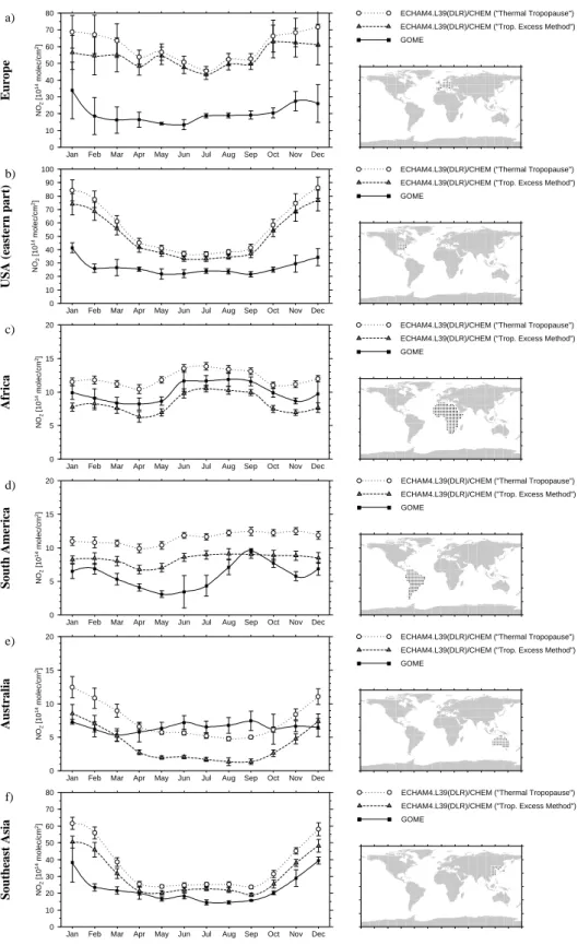
Figure 4 shows the results of the regional comparison. These can be summarized as follows:
– For the region ‘Europe’, E39/C and GOME show
0 10 20 30 40 50 60 70 80 NO 2 [10 14 molec/cm 2]
Jan Feb Mar Apr May Jun Jul Aug Sep Oct Nov Dec
Europe
a) ECHAM4.L39(DLR)/CHEM ("Thermal Tropopause")
ECHAM4.L39(DLR)/CHEM ("Trop. Excess Method") GOME 0 10 20 30 40 50 60 70 80 90 100 NO 2 [10 14 molec/cm 2]
Jan Feb Mar Apr May Jun Jul Aug Sep Oct Nov Dec
USA (eastern part)
b) ECHAM4.L39(DLR)/CHEM ("Thermal Tropopause")
ECHAM4.L39(DLR)/CHEM ("Trop. Excess Method") GOME 0 5 10 15 20 NO 2 [10 14 molec/cm 2]
Jan Feb Mar Apr May Jun Jul Aug Sep Oct Nov Dec
Africa
c) ECHAM4.L39(DLR)/CHEM ("Thermal Tropopause")
ECHAM4.L39(DLR)/CHEM ("Trop. Excess Method") GOME 0 5 10 15 20 NO 2 [10 14 molec/cm 2]
Jan Feb Mar Apr May Jun Jul Aug Sep Oct Nov Dec
South America
d) ECHAM4.L39(DLR)/CHEM ("Thermal Tropopause")
ECHAM4.L39(DLR)/CHEM ("Trop. Excess Method") GOME 0 5 10 15 20 NO 2 [10 14 molec/cm 2]
Jan Feb Mar Apr May Jun Jul Aug Sep Oct Nov Dec
Australia
e) ECHAM4.L39(DLR)/CHEM ("Thermal Tropopause")
ECHAM4.L39(DLR)/CHEM ("Trop. Excess Method") GOME 0 10 20 30 40 50 60 70 80 NO 2 [10 14 molec/cm 2]
Jan Feb Mar Apr May Jun Jul Aug Sep Oct Nov Dec
Southeast Asia
f) ECHAM4.L39(DLR)/CHEM ("Thermal Tropopause")
ECHAM4.L39(DLR)/CHEM ("Trop. Excess Method") GOME
Fig. 4. (a – f): Seasonal variation of the tropospheric NO2column amounts for the climatological average values for selected spatial domains. The two sigma standard deviation of the individual monthly means to the climatological monthly means are drawn as errorbars for each data point. The small map to the right depicts the grid cells, that have been used to calculate the average values of the specified domain.
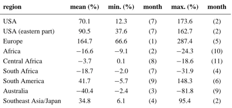
Table 3. Summary of the minimum, maximum and mean relative differences r (given by Eq. 1) of the average values of the tropospheric NO2column amounts for the selected source regions. Positive (negative) values are corresponding to larger (smaller) column amounts by
E39/C
region mean (%) min. (%) month max. (%) month
USA 70.1 12.3 (7) 173.6 (2)
USA (eastern part) 90.5 37.6 (7) 162.7 (2)
Europe 164.7 66.6 (1) 287.4 (5) Africa −16.6 −9.1 (2) −24.3 (10) Central Africa −3.7 0.1 (8) −18.6 (11) South Africa −18.7 −2.0 (7) −31.9 (4) South America 41.7 −5.7 (9) 148.3 (6) Australia −40.4 −2.4 (3) −81.8 (9) Southeast Asia/Japan 34.8 6.1 (4) 95.4 (2)
results of E39/C (“TEM”) is 2.65 times greater than that of GOME (Fig. 4a).
– In contrast to the GOME data, the model produces a
rel-atively large and distinctive seasonal variation in the re-gions ‘USA’ (not shown) and ‘(eastern) USA’ (Fig. 4b): maximum values occurring during the winter and min-imum values during the summer. The results of E39/C show higher column amounts than the GOME data dur-ing the whole year, the annual mean is 1.7 times (USA) resp. 1.9 times ((eastern) USA) greater than that of GOME.
– The tropospheric NO2 column amounts of E39/C and GOME for the region ‘Africa’ are both qualitatively and quantitatively similar. The annual mean of the GOME data is 1.2 times higher than that of E39/C (“TEM”) (Fig. 4c).
– The tropospheric TEM NO2 column amounts from GOME exhibit a distinctive seasonal variation for the region ‘South America’, having a minimum in May and a maximum in September. This is not reproduced by E39/C which shows only small seasonal variations. The annual mean of E39/C is 1.4 times greater than that of GOME (Fig. 4d).
– In ‘Australia’, the TEM NO2column data from GOME
exhibit only a small seasonal variation, whereas E39/C shows a distinctive seasonal variation with minimum values occurring in winter and maximum values in sum-mer. In contrast to the other regions, the model shows noticeably less NO2than the measurements during the
winter months, when lightning activity is at its mini-mum. As lightning produced NOx is dominating the
seasonal variation of the NOx emissions in the model
(and therefore the seasonal variation of the tropospheric
NO2column amounts), lightning produced NOxseems
to be well represented by E39/C as there is good agree-ment between model and measureagree-ments during summer when the lightning activity is high. However, the other NOxsources seem to be too weak, particularly in
win-ter. This could explain why the modelled NO2column
amounts have lower values than the measured ones dur-ing the Australian winter. The annual mean of GOME is 1.7 times greater than that of E39/C (Fig. 4e).
– For the region ‘Southeast Asia/Japan’, the tropospheric
NO2column amounts of E39/C and GOME are in good
agreement. The only striking discrepancy is the month of February. Whereas the values of GOME go down rapidly from January to February, the decrease between January and February is shown by E39/C to a much lesser extent. The annual mean of E39/C is slightly higher than that of GOME, the relative difference being about 35% (Fig. 4f).
Table 3 summarizes the minimum, maximum and average relative difference of the TEM modelled and retrieved tropo-spheric NO2column amounts by E39/C and GOME,
respec-tively. The relative difference r is calculated by Eq. (1):
r =
0E39/C (TEM)0−0GOME0
0GOME0 ·100% (1)
4 Discussion of results
There are several possible reasons for the observed differ-ences between model and measurements. These can be di-vided into three basic error classes:
– errors from the GOME measurements and from the
derivation of the tropospheric column amounts of the measured spectra,
– differences arising in the generation of the two data
sources.
4.1 Model errors and deficiencies
How accurate and representative the model output is, depends on:
– the description of the atmospheric dynamics; – the chemical scheme;
– the accuracy of the input data; – the initialization data.
As NO2 has a relatively short chemical short lifetime, the
description of its chemical production and loss and the dis-tribution and magnitude of sources are of significance.
The input sources are based on monthly means, which are assumed to remain constant during the whole period of simu-lation (20 years), except for lightning produced NOxwhich is
related to the model’s cloud parameterization scheme (Hein et al., 2001).
One of the main uncertainties in the calculated NOx
vol-ume mixing ratios, which are the basis for the calculation of the tropospheric NO2column amounts, are the
uncertain-ties of the NOxemissions, both in the total amount and in
the seasonal variation. Here, a simple phase shift of the used biomass burning dataset in the southern hemisphere (particularly South America and South Africa) by about one month could possibly improve the agreement of the modelled and observed seasonal variation of E39/C and GOME sig-nificantly (Lauer, 2001). In contrast, the seasonal variation of the biomass burning data set in (Northern) and Central Africa, which is dominating the seasonal variation of the to-tal NOxemissions in this region seems to be quite good as
the seasonal variation of the modelled and the observed tro-pospheric NO2column amounts are in good agreement.
In Australia, very low values of the NO2column amounts
are modelled. As a direct result of the uncertainties of the emissions, the modelled tropospheric NO2has large
uncer-tainties. Here, even slight changes of the emissions could give a different seasonal variation. Nevertheless, in summer when the lightning activity is high in Australia, there is good agreement between the two datasets both in the seasonal vari-ation and in the absolute values for the column amounts. As the seasonal variation of the modelled NO2column amounts
is clearly dominated by the lightning produced NOx
emis-sions, the modelled lightning produced NOxseems to be
ap-propriate. In addition to the general uncertainties of the NOx
emissions, the datasets employed in the model have no daily variation, as e.g. caused by the rush hour in the morning and evening in Europe or the United States.
Even more important is the missing VOC chemistry and the missing NOx sink process ‘heterogeneous reaction of
N2O5 with H2O forming HNO3’ on the surface of
tropo-spheric aerosols and at the Earth’s surface.
The missing VOC chemistry prevents the formation of the NOxreservoir species PAN. A model study by Kuhn (1996)
examined the impact of PAN on the NOxmixing ratios using
the global 3-D Chemical Tracer Model, CTM, which has a horizontal resolution of 4◦×5◦and 9 vertical layers extend-ing from the surface up to 10 hPa. Two model simulations, with and without taking into account PAN, were compared. The results showed, that PAN decreases (increases) the NOx
mixing ratio in regions with high (low) NOx mixing ratio,
e.g. above the continents (oceans). However, the results sug-gest the effect on the NOxmixing ratio is below 10% above
continents (Kuhn, 1996), and therefore probably even less on the tropospheric NO2column amounts.
In contrast, the missing hydrolysis of N2O5 on
tropo-spheric aerosols seems to be quite important, especially for the mid-latitudes. Dentener and Crutzen (1993) studied the impact of the reaction of N2O5 on tropospheric aerosols
on the global distributions of NOx, O3 and OH using the
global 3-D chemical tracer model Moguntia, which has a horizontal resolution of 10◦×10◦ and 10 vertical layers at 100 hPa distance. They took into account the role of night time chemical reactions of NO3 and N2O5 on aerosol
sur-faces and calculated the resulting loss in NOx. Their
re-sults showed that this additional NOxsink reduces the NOX
(NOX = NO + NO2+NO3+N2O5+HNO4) present in
the boundary layer above the U.S. and Europe by about 50% in winter and about 20% in summer. The increased hetero-geneous NOX removal in winter is due to long darkness and low temperatures during the winter months. For tropical re-gions, e.g. Africa, this process seems to be much less im-portant and reduces the boundary layer NOX only about 10 to 30%. This can be explained by the increased importance of the daytime reaction of NO2with OH in tropical regions
(Dentener and Crutzen, 1993).
In contrast, a study by Schultz et al. (2000) analysing aircraft measurements at 6–12 km altitude over the tropical South Pacific states that the N2O5hydrolysis is less
impor-tant (in the free troposphere over the tropical South Pacific) than previously assumed by other (modeling) studies. How-ever, this is not contradictory to the conclusion of this study (based on the study of Dentener and Crutzen, 1993) on the effect of the N2O5hydrolysis on the tropospheric NO2
col-umn amounts, as the major fraction of the tropospheric NO2
column amounts is located in the boundary layer and lower troposphere and not in the free troposphere.
In Europe, North America and Asia, large quantities of NOxare released in winter into the planetary boundary layer.
In the tropics convective activity pumps some of the NOx
out of the planetary boundary layer and the lightning source releases NOxabove the planetary boundary layer, where the
The current limitations within the model, describing the NOxemissions and the chemistry in the lower troposphere,
appear strong candidates to explain the differences between model and retrieved datasets. Particularly the missing N2O5
hydrolysis should account for some of the overestimation of NO2by the model. The estimated size of the error (as stated
by Dentener and Crutzen, 1993) is in good agreement with the observed differences.
4.2 GOME errors
Errors are introduced to the TEM NO2column dataset from
GOME observations for two types of reason:
– Inherent uncertainties in the measurement itself and the
retrieval of the trace gas concentration from the mea-sured spectra.
– Remote sensing specific issues.
The errors from the measurement and the retrieval using DOAS are small in general and can usually be neglected compared to the other error sources.
In contrast, the errors due to remote-sensing specific prob-lems are potentially more significant. To detect NO2, GOME
measures visible light (425 to 450 nm). The presence of clouds prevents the detection of NO2 below the cloud, and
enhances GOME’s sensitivity for the detection of NO2above
the cloud top. To minimize the impact of clouds, the retrieval of the TEM tropospheric NO2column amounts is restricted
to atmospheric scenes having a cloud coverage below the threshold value 10%. This threshold value has been chosen to balance between meeting the needs of the ‘clear sky’ as-sumption in the AMF calculations and the number of avail-able measurements. Because of the large dimension of the GOME pixels, the number of usable measurements would drop dramatically when using a lower threshold value.
Errors arising from undetected clouds (i.e. sub pixel scene) and cloud fractions below the threshold value may lead to an underestimation of tropospheric NO2by up to 40%,
al-though in most cases, this error is well below this peak value (Richter and Burrows, 2001). The presence of large amounts of aerosols have a similar effect on the detection of NO2as
clouds.
A study by Martin et al. (2001) showed the potential of further improvements on the retrieval of tropospheric NO2
from the GOME measurements. A new approach of using a global 3-D model of tropospheric chemistry for the calcu-lation of the vertical NO2 profiles required to calculate the
AMF instead of assuming a globally uniform vertical profile seems to improve the NO2retrieval. In addition, especially
the new treatment of partly cloudy scenes should improve the retrieval of tropospheric NO2. This new AMF
formula-tion enables the quantitative retrieval for partly cloudy scenes (which is the case quite often because of the large dimensions of the individual GOME pixels) (Martin et al., 2001).
In addition, also the separation of the total column amounts into stratospheric and tropospheric part are a poten-tial error source as additional assumptions have to be made. In order to see the effect on the tropospheric NO2column
amounts of this method of calculation, the model data have been calculated using “TEM” as well.
4.3 Different assumptions in the creation of the two datasets
There are three major sources, which may result in differ-ences when comparing the model- and satellite data and arise from differences in their:
– Temporal offset,
– exclusive use of clear sky conditions, – sun synchronous orbit of ERS-2.
As mentioned above, all the input conditions used for the model runs are representative of the early 1990s, whereas the GOME measurements were taken between 1996 and 2000. Thus a temporal offset of several years exists between the periods represented by the model and measured by GOME. Changes of the anthropogenic NOx emissions resulting in
different NO2 concentrations might in part also explain the
differences. However the uncertainties on the NOxemission
datasets used as input for the model are in any case large (see Table 2).
For the GOME data, only clear sky (threshold value for the cloud coverage of 10%) pixels are accounted for. In contrast, the tropospheric NO2column amounts from the model
out-put have been calculated without taking cloud effects or the cloud fraction within the model box explicitly into account.
The loss of NOx by the reaction of N2O5on aerosol and
on cloud, which is significant at night, has been discussed above. In addition as NO2is photolysed by the incoming
so-lar ultraviolet radiation, the lack of cloud in the model and presence of some cloud in the measurement is likely to im-pact on the comparison. This effect is difficult to quantify, too, because of the large dimensions of the model boxes, only very few data points will remain after sorting out all values with a cloud fraction above 10%. Especially for the mid-latitudes, it might become impossible to calculate repre-sentative monthly means.
The probably most important fact making the compari-son of the model- and satellite data difficult is the sun syn-chronous orbit of GOME’s space platform, the ERS-2 satel-lite. Because of this, every measurement of GOME is per-formed at the same local time between 10:05 and 10:55 LT. This period coincides with the minimum of the daily light-ning activity over the continents as shown by long term ob-servations of the Optical Transient Detector, OTD (Kurz, 2001). The simulation E39/C only provides averaged NO2
values. Thus the modelled 24 hours average of the lightning produced NOxwill overestimate the NOxpresent in the late
morning. A 3-D chemical transport model study by Velders et al. (2001) indicates that the NO2tropospheric columns at
10:30 LT are about 80% of the values averaged over 24 hours for the region Europe and the U.S., about 50 to 70% for the regions South America and Africa.
5 Conclusions
Overall the differences in the NO2tropospheric columns as
retrieved from GOME observations and calculated by the general circulation model E39/C are within a factor of 2 to 3. The likely overestimation of the NOxin the GCM is
prob-ably best explained by the lack of the heterogeneous loss of NOxthrough the reaction of N2O5with H2O on aerosols and
clouds in the lower troposphere. Thus, extending the chem-istry module CHEM to properly handle the heterogeneous N2O5chemistry should be the next step in improving E39/C
to perform simulations of tropospheric NOx.
In spite of the deficiencies and various error sources of both model and satellite data, this investigation shows clearly the potential for testing the current capability of general cir-culation models to simulate the behaviour of the troposphere using satellite observations.
The major features of this first look can be summarized as follows:
In the northern mid-latitudes (USA, Europe), emissions from industry and ground based traffic are the most impor-tant source for NOx.
In the tropics, especially biomass burning and emissions from lightning are the dominant NOxsources. Here, the
sea-sonal variation, as well as the quantitative column amounts are in better agreement than for the USA and Europe. This is consistent with the conclusion of Dentener and Crutzen (1993) stating much lesser influence of the still missing ad-ditional NOx sink in the tropics. The better agreement in
these regions also indicates that the prescribed biomass burn-ing and lightnburn-ing produced NOxemissions are quite
reason-able.
Acknowledgements. This work is a contribution to TROPOSAT
(EUROTRAC-2). It has been funded in part by the University and State of Bremen, the Ludwig-Maximilians-University M¨unchen, the German Aerospace Center (DLR) and the European Union through the TRADEOFF and POET projects. The provision of level 1 GOME data by ESA for this scientific study is acknowl-edged.
References
Benkovitz, C. M., Scholtz, M. T. , Pacyana, J., Tarrason, L., Dignon, J, Voldner, E. C., Spiro, P. A., Logan, J. A., and Graedel, T. E.: Global gridded inventories of anthropogenic emissions of sulfur and nitrogen, J. Geophys. Res., 101(D), 29 239–29 253, 1996. Bradshaw, J., Davis, D., Grodzinsky, G., Smyth, S., Newell, R.,
Sandholm, S., and Liu, S.: Observed distributions of nitrogen
oxides in the remote free troposphere from the NASA Global Tropospheric Experiment programs, Rev. Geophys., 38, 61–116, 2000.
Brasseur, G. P., Orlando, J. J., and Tyndall, G. S.: Atmospheric Chemistry and Global Change, Oxford Univ Pr (Sd), ISBN 0195105214, 1999.
Burrows, J. P., Weber, M., Buchwitz, M., Rozanov, V., Ladst¨atter-Weißenmayer, A., Richter, A., DeBeek, R., Hoogen, R., Bram-stedt, K., Eichmann, K. -U., Eisinger, M., and Perner, D.: The Global Ozone Monitoring Experiment (GOME): Mission Con-cept and First Scientific Results, J. Atmos. Sci., 56, 151–175, 1999.
Dentener, F. J. and Crutzen, P. J.: Reaction of N2O5 on
Tropo-spheric Aerosols: Impact on the Global Distributions of NOx,
O3and OH, J. Geophys. Res., 98(D4), 7149–7163, 1993.
EPA (United States Environmental Protection Agency): Air Quality Index – A Guide to Air Quality and Your Health, Washington D. C., 20460, EPA-454/R-00-005, 2000.
ESA (European Space Agency): GOME Global Ozone Monitoring Experiment users manual, ESA SP-1182, ESA/ESTEC, Noord-wijk, Netherlands, ISBN 92-9092-327-x, 1995.
Finlayson-Pitts, B. J. and Pitts, J. N., Jr.: Chemistry of the Upper and Lower Atmosphere, Academic Press, ISBN 012257060X, 1999.
Hao, W. M., Liu, M.-H., and Crutzen, P. J.: Estimates of annual and regional releases of CO2and other traces gases to the atmosphere from fires in the tropics, based on the FAO statistics for the pe-riod 1975–1980, in Fire in the Tropical Biota, Ecological Studies, Vol. 84, (Ed) Goldammer, J. G., 440–462, Springer-Verlag, New York, 1990.
Hein, R., Dameris, M., Schnadt, C., Land, C., Grewe, V., K¨ohler, I., Ponater, M., Sausen, R., Steil, B., Landgraf, J., and Br¨uhl, C.: Results of an interactively coupled atmospheric chemistry-general circulation model: Comparison with observations, Ann. Geophysicae, 19, 435–457, 2001.
Jones, A. E., Weller, R., Anderson, P. S., Jacobi, H.-W., Wolff, E. W., and Schrems, O.: Measurements of NOxemissions from
Antarctic snowpack, Geophys. Res. Lett., 28, 1499–1502, 2001. Kuhn, M.: Untersuchungen zur troposph¨arischen Verteilung von Stickoxiden, Ozon, OH, Peroxiden, Aldehyden und PAN mit einem dreidimensionalen globalen Chemie- und Trans-portmodell, Ph.D. thesis, Mathematisch-Naturwissenschaftliche Fakult¨at der Universit¨at zu K¨oln, K¨oln, 1996.
Kurz, C.: NOx-Produktion durch Blitze und die Auswirkung auf
die globale Chemie der Atmosph¨are, diploma thesis, Meteorolo-gisches Institut der Universit¨at M¨unchen, M¨unchen, 2001. Land, C., Ponater, M., Sausen, R., and Roeckner, E.: The
ECHAM4.L39(DLR) atmosphere GCM – Technical description and model climatology, Report No. 1991-31, DLR Oberpfaffen-hofen, Wessling, Germany, ISSN 1434-8454, 1999.
Lauer, A.: Untersuchungen der geographischen und jahreszeitlichen Variationen von troposph¨arischen NO2 S¨aulen
– Vergleich von Modell- und Satellitendaten, diploma thesis, Meteorologisches Institut der Universit¨at M¨unchen, M¨unchen, 2001.
Lee, D. S., K¨ohler, I., Grobler, E., Rohrer, F., Sausen, R., Gallardo-Klenner, L., Olivier, J. G. J., Dentener, F. J., and Bouwman, A. F.: Estimations of global NOxemissions and their uncertainties,
Leue, C., Wenig, M., Wagner, T., Klimm, O., Platt, U., and J¨ahne, B.: Quantitative analysis of NOxemissions from Global Ozone
Monitoring Experiment satellite image sequences, J. Geophys. Res., 106, 5493–5505, 2001.
Martin, R. V., Chance, K., Jacob, D. J., Kurosu, T. P., Spurr, R. J. D., Bucsela, E., Gleason, J. F., Palmer, P. I., Bey, I., Fiore, A. M., Li, Q., and Yantosca, R. M.: An Improved Retrieval of Tropospheric Nitrogen Dioxide from GOME, submitted to J. Geophys. Res., 2001.
Price, C. and Rind, D.: A Simple Lightning Parameterization for Calculating Global Lightning Distributions, J. Geophys. Res., 97(D), 9919–9933, 1992.
Richter, A. and Burrows, J. P.: Tropospheric NO2 from GOME
measurements, Adv. Space Res., in press, 2001.
Schmitt, A. and Brunner, B.: Emissions from aviation and their de-velopment over time, in Pollutants from air traffic – results of atmospheric research 1992-1997, DLR-Mitt. 97-04, (Eds) Schu-mann, U., et al., 37–52, DLR K¨oln, 1997.
Schnadt, C., Dameris, M., Ponater, M., Hein, R., Grewe, V., and Steil, B.: Interaction of atmospheric chemistry and climate and its impact on stratospheric ozone, Clim. Dyn., in press, 2001. Schultz, M. G., Jacob, D. J., Wang, Y., Logan, J. A., Atlas, E. L.,
Blake, D. R., Blake, N. J., Bradshaw J. D., Browell, E. V., Fenn, M. A., Flocke, F., Gregory, G. L., Heikes, B. G., Sachse, G. W., Sandholm, S. T., Shetter, R. E., Singh, H. B., and Talbot, R. W.: On the origin of tropospheric ozone and NOxover the tropical
South Pacific, J. Geophys. Res., 104, 5 829–5 843, 1999. Schultz, M. G., Jacob, D. J., Bradshaw, J. D., Sandholm, S. T., Dibb,
E. J., Talbot, R. W., and Singh, H. B.: Chemical NOxbudget in
the upper troposphere over the tropical South Pacific, J. Geophys. Res., 105, 6 669–6 679, 2000.
Steil, B., Dameris, M., Br¨uhl, C., Crutzen, P. J., Grewe, V., Ponater, M., and Sausen, R.: Development of a chemistry module for GCMs: first results of a multiannual integration, Ann. Geophys-icae, 16, 205–228, 1998.
Velders, G. J. M., Granier, C., Portmann, R. W., Pfeilsticker, K., Wenig, M., Wagner, T., Platt, U., Richter, A., and Burrows, J. P.: Global tropospheric NO2column distributions: Comparing 3-D
model calculations with GOME measurements, J. Geophys. Res., 106, 12 643–12 660, 2001.
Wayne, R. P. (Ed): The nitrate radical: physics, chemistry, and the atmosphere, Atmos. Environ., 25, 1–203, 1991.
Yienger, J. J. and Levy, H.: Empirical model of global soil-biogenic NOxemissions, J. Geophys. Res., 100(D), 11 447–11 464, 1995.