HAL Id: hal-02989914
https://hal-amu.archives-ouvertes.fr/hal-02989914
Submitted on 6 Nov 2020
HAL is a multi-disciplinary open access archive for the deposit and dissemination of sci-entific research documents, whether they are pub-lished or not. The documents may come from teaching and research institutions in France or abroad, or from public or private research centers.
L’archive ouverte pluridisciplinaire HAL, est destinée au dépôt et à la diffusion de documents scientifiques de niveau recherche, publiés ou non, émanant des établissements d’enseignement et de recherche français ou étrangers, des laboratoires publics ou privés.
geochemical proxies from marine sediments:
implications for model-data comparisons
Guillaume Leduc, Thibault Garidel-Thoron, Jérôme Kaiser, Clara Bolton,
Camille Contoux
To cite this version:
Guillaume Leduc, Thibault Garidel-Thoron, Jérôme Kaiser, Clara Bolton, Camille Contoux. Databases for sea surface paleotemperature based on geochemical proxies from marine sediments: implications for model-data comparisons. Quaternaire, AFEQ-CNF INQUA, 2017, pp.201 - 216. �10.4000/quaternaire.8034�. �hal-02989914�
Revue de l'Association française pour l'étude du Quaternaire
vol. 28/2 | 2017
Volume 28 Numéro 2
Databases for sea surface paleotemperature based
on geochemical proxies from marine sediments:
implications for model-data comparisons
Bases de données des paléotempératures de l’océan de surface issues des proxies
géochimiques analysés sur les sédiments marins : implications pour les
comparaisons modèles-données
Guillaume Leduc, Thibault de Garidel‑Thoron, Jérôme Kaiser, Clara Bolton and Camille Contoux
Electronic version
URL: http://quaternaire.revues.org/8034 DOI: 10.4000/quaternaire.8034 ISSN: 1965-0795
Publisher
Association française pour l’étude du quaternaire
Printed version
Date of publication: 29 May 2017 Number of pages: 201-216 ISSN: 1142-2904
Brought to you by Aix-Marseille Université
Electronic reference
Guillaume Leduc, Thibault de Garidel‑Thoron, Jérôme Kaiser, Clara Bolton and Camille Contoux, « Databases for sea surface paleotemperature based on geochemical proxies from marine sediments: implications for model-data comparisons », Quaternaire [Online], vol. 28/2 | 2017, Online since 01 June 2017, connection on 04 September 2017. URL : http://quaternaire.revues.org/8034 ; DOI : 10.4000/ quaternaire.8034
Manuscrit reçu le 20/01/2017, accepté le 21/03/2017
DATABASES FOR SEA SURFACE PALEOTEMPERATURE
BASED ON GEOCHEMICAL PROXIES FROM MARINE SEDIMENTS:
IMPLICATIONS FOR MODEL-DATA COMPARISONS
n
Guillaume LEDUC
1, Thibault de GARIDEL-THORON
1, Jérôme KAISER
2,
Clara BOLTON
1& Camille CONTOUX
1ABSTRACT
The Paleoclimate Model Intercomparison Project (PMIP) aims to simulate the response of Earth’s climate system to changes in different climate forcing factors, focusing on six key intervals of the geological past (the mid-Piacenzian Warm Period at ~3.3-3.0 Ma, the last interglacial period at ~127 ka, the last glacial maximum at ~21 ka, the mid-Holocene at ~6 ka, the last millennium i.e. the 850-1850 Common Era (CE) time window, as well as the last glacial termination, i.e. the ~21-9 ka time window). Model evaluation is ultimately achieved via model-data comparison exercises, and such diagnoses rely on databases of proxy-based paleoclimate recons-tructions available in the literature. In this context, we provide a review of the main geochemical sea surface temperature (SST)
proxies (namely foraminiferal Mg/Ca ratio, the UK’
37, and the TEX86) that are routinely used to aliment databases used in model-data
comparisons, focusing on proxy systematics and specificities that may affect or bias SSTs reconstructed with each of these proxies. We then go on to discuss notorious mismatches between SST estimates derived from different proxies for all periods studied in PMIP, and aim to provide guidance for a better interpretation of these model-data mismatches. This review is deliberately aimed at helping the paleoclimate modeling community to better appraise how information on past SST variability is transferred to the marine geolo-gical record. In particular, when SST estimates based on different proxies provide contrasting SST signals, we stress the importance of looking at those contrasting signals through the prism of the ecology of the organisms at the origin of the SST proxies.
Keywords : Paleoclimate Model Intercomparison Project (PMIP), Sea Surface Temperature (SST), Databases, foraminiferal Mg/Ca,
Alkenone unsaturation index (UK’
37), Tetraether index 86, (TEX86)
RÉSUMÉ
BASES DE DONNÉES DES PALÉOTEMPÉRATURES DE L’OCÉAN DE SURFACE ISSUES DES PROXIES GÉOCHIMIQUES ANALYSÉS SUR LES SÉDIMENTS MARINS : IMPLICATIONS POUR LES COMPARAISONS MODÈLES-DONNÉES
Le Projet d’intercomparaison des modèles des paléoclimats (PMIP) vise à simuler la réponse du système climatique terrestre aux changements des différents facteurs de forçage du climat, en se concentrant sur six intervalles clés du passé géologique : la période chaude du Plaisancien moyen il y a environ 3,3-3,0 Ma, la dernière période interglaciaire à ~127 ka, le dernier maximum glaciaire à ~21 ka, l’Holocène moyen à ~6 ka, le dernier millénaire, c’est-à-dire la fenêtre de temps 850-1850 Common Era (CE), ainsi que la dernière terminaison glaciaire, c’est-à-dire la fenêtre de temps entre 21 et 9 ka. L’évaluation des modèles est réalisée par des comparaisons modèles-données, et de tels diagnostics reposent sur des bases de données de reconstructions paléoclimatiques basées sur les traceurs disponibles dans la littérature. Dans ce contexte, nous passons en revue les principaux traceurs géochimiques
pour l’estimation des températures de surface de la mer (SST), à savoir le rapport Mg/Ca des foraminifères, l’UK’
37 et le TEX86 qui
sont couramment utilisés pour alimenter les bases de données utilisées dans les comparaisons modèles-données. En se concentrant sur les spécificités des traceurs qui peuvent affecter ou biaiser les reconstructions de SST, nous discuterons ensuite des principales disparités entre les estimations de SST dérivées de différents traceurs et des modélisations des SST pour toutes les périodes étudiées dans le programme PMIP, et tenterons de fournir des indications pour mieux interpréter ces différences. Cette revue de l’état de l’art a pour objectif d’aider la communauté des modélisateurs à mieux comprendre les principales sources d’incertitudes des estimations de paléotempératures dérivées des archives sédimentaires océaniques. En particulier, lorsque les estimations de SST basées sur des traceurs différents fournissent des signaux SST divergents, nous soulignons l’importance de regarder ces signaux contrastés au travers du prisme de l’écologie des organismes à l’origine des traceurs de SST.
Mots-clés : Projet d’intercomparaison de la modélisation des paléoclimats (PMIP), températures océaniques de surface (SST), bases
de données, Mg/Ca des foraminifères, index d’insaturation des alcénones (UK37’), index tetraether 86 (TEX
86)
1 Aix-Marseille Université, CNRS, IRD, Collège de France, Centre Européen de Recherche et d’Enseignement de Géosciences de
l’Environnement (CEREGE), UM34, Europole Méditerranéen de l’Arbois, BP 80, 13545 AIX-EN-PROVENCE, France.
Courriel : [email protected], [email protected], [email protected], [email protected]
2 Leibniz Institute for Baltic Sea Research (IOW), Marine Geology, Seestrasse 15, 18119, ROSTOCK-WARNEMÜNDE, Germany.
1 - INTRODUCTION
Since the middle of the 19th century, anthropogenic activities have driven the Earth’s climate away from its pre-industrial background state (Abram et al., 2016; IPCC, 2013). In this context, assessments of population or ecosystem vulnerability and adaptation strategies exclusi-vely rely on climate model projections driven by different emissions scenarii. Over the last two decades, the climate modelling community has been working to evaluate the performance of climate models in the framework of the Paleoclimate Model Intercomparison Project (PMIP), through simulations of past climate background states and comparison of the modelling outputs to paleocli-mate reconstructions (see Kageyama et al., 2016 for an introduction of the fourth PMIP phase). The ongoing PMIP4 project will ultimately provide model outputs for 5 time slices: the Mid-Piacenzian Warm Period (mPWP, i.e. at ~3.3-3.0 Ma), the last interglacial period (LIG, i.e. at ~127 ka), the last glacial maximum (LGM, i.e. at ~21 ka), the mid-Holocene (MH, i.e. at ~6 ka) and the last millennium (LM, i.e. the 850-1850 CE time window) (Kageyama et al., 2016), as well as a series of transient simulations of the last glacial termination (LGT, i.e. the ~21-9 ka time window) (Ivanovic et al., 2016).
The model evaluation step requires researchers to compare model outputs to quality-controlled paleo-climatic databases compiling different metrics of past climates. Such paleoclimatic databases provide bench-marks for assessing climate models’ skills. In those data-bases, the measurements of past oceanic changes are based on “proxies”, that can be defined as “measurable descriptors for desired but unobservable environmental variables”, such as SST in the case considered here (Wefer et al., 1999). The main metrics of past climatic change in the ocean is the sea surface temperature (SST), which has been the focus of many studies. Over the last few decades, numerous databases were assembled to reconstruct global continental temperature and SST fields during the relevant PMIP time-slices. Although the modelling community has made a sustained effort to perform this model evaluation (see e.g. Kageyama et al., 2013), paleoceanographers are lagging behind in terms of producing extensive evaluation of databases with respect to geochemical and micropaleontological proxies for SST. Such a lag in paleoclimate database evaluation is partly due to the difficulties involved in compiling data from a mosaic of different proxies, each with their own specificities which are not always easy to objectively evaluate within a single database. For example, paleo-thermometers based on biomarkers such as the C37 alke-none unsaturation index (UK’
37) and the Tetraether indEX
with 86 carbon atoms (TEX86) cannot easily be assigned to specific seasons and/or water depths because the biomarkers used in those two proxies are synthesized by different species of phytoplanktonic algae (for the UK’
37)
and of archaea (for the TEX86). In contrast, the seasonal and water depth preferences embedded in species-specific foraminiferal Mg/Ca can often be evaluated in the modern ocean using sediment traps that collect
particles sinking through the water column (Jonkers & Kucera, 2015), or with ecophysiological models that take into account the ecology of foraminifers (Lombard et al., 2011). Besides ecological preferences, different geoche-mical proxies have also their own specific biases (see discussion in Chapter 2), complicating the comparison of multiproxy databases to model outputs.
Here we provide a brief overview of geochemical SST proxies used in SST compilations for some selected time windows relevant to the PMIP project. The objective is to provide guidance for model-data comparison studies, in particular to the modeling community who might lack a deep understanding on how and why individual SST esti-mates might deviate from the mean-annual SST estimate often provided in SST databases. We will highlight some notable model-data mismatches and suggest possible scenarii to reconcile them in light of each geochemical proxy’s specificities.
2 - A BRIEF OVERVIEW OF GEOCHEMICAL SST PROXIES
Paleoceanographic proxies for SST derived from marine sediments exclusively rely on organic or inorganic remains of marine organisms (archaea, phytoplank ton or zooplankton) that are assumed to have lived at the ocean surface (i.e. the mixed layer), or slightly below the ocean surface (i.e. in subsurface). After the death of these orga-nisms, their remains sink to the seafloor (often inside fecal pellets or in the form of aggregates called “marine snow”) and are buried in the sediments, making sedimen-tary sequences suitable archives for past SST reconstruc-tion once a chronology is available.
The first attempts to estimate past SST were based on planktonic microfossil assemblages. As different plan-ktonic species have different ecological niches, their spatial distributions in the ocean depend on environ-mental parameters such as temperature, salinity and food availability. In such approaches, near-modern assem-blages of planktonic organisms counted in surface sedi-ments are calibrated against one or several chosen surface or subsurface ocean properties. Because SST is the main factor controlling modern assemblages in the global ocean, it is possible to infer past SST by reconstructing downcore changes in species’ abundances through the use of statistical methods (Imbrie & Kipp, 1971; see also Mix et al., 1999 and Kucera et al., 2009 and references therein for more details on faunal assemblage tech-niques). Although extremely valuable, the main pitfall of statistical estimates of past temperatures based on assemblages is the occurrence of species or assemblages in the fossil record that have no modern analogs – the so-called no-analog problem. Geochemical proxies, often based on thermodynamic processes, do not suffer from this problem and can therefore be used to extrapolate past conditions outside of the modern ocean range once they are carefully calibrated. Moreover, geochemical proxies can be calibrated in vitro, whereas this is not possible for assemblage-based proxies.
Since the 1980s, new geochemical tools have been developed to reconstruct past SST that do not rely on assemblages. These proxies do not always provide the same SST estimates as faunal or floral assemblages techniques (see Bard, 2000), and have subsequently increasingly been incorporated into SST databases. Now that geochemical SST proxies are widely integrated in databases, comparing different SST estimates based on different proxies in contrasting oceanic regimes can help refine our understanding of both paleotemperatures and SST proxy specificities. Below, we concisely review the three most commonly used geochemical proxies for past SST derived from marine sediments.
2.1 - FORAMINIFERAL MG/CA
Planktonic foraminifera are unicellular zooplan-kton protists that precipitate shells – or tests – made of calcium carbonate (CaCO3). Ca can be substituted by Mg in the carbonate lattice, and early suggestions of a thermo-dependence of Mg incorporation were first made in the early 1970s (Kilbourne & Sen Gupta, 1973; Bender et al., 1975). Two decades later, analysis of fora-minifera cultured at laboratory unambiguously demons-trated that foraminiferal test Mg/Ca is thermo-dependent, paving the way to the use of foraminiferal Mg/Ca as a paleothermometer (Nürnberg et al., 1996). Later, further culture experiments complemented by core-top analyses and sediment trap studies demonstrated that Mg/Ca exponentially increases with the ambient temperature at which planktonic foraminifera calcify (see Dekens
et al., 2002; Anand et al., 2003 among many others).
Since the mid 1990s, a wealth of calibration equations has been published, which vary significantly with ocean basin and foraminifera species used for paleotemperature reconstructions (see e.g. McConnell & Thunell, 2005, Regenberg et al., 2009). Those calibration efforts further refined the accuracy of SST estimates, even though most calibration equations use a similar slope within the cali-bration uncertainty. Such a variety of calicali-brations poses a challenge in assembling SST databases since they may contribute to increase SST heterogeneities or require to re-calibrate raw Mg/Ca values when new calibrations become available.
Other effects, such as salinity and foraminiferal disso-lution have been identified as secondary effects on the Mg/Ca signature of planktonic foraminifera. For example, high salinity may increase Mg/Ca independently of temperature (Kisakürek et al., 2008; Mathien-Blard & Bassinot, 2009; Arbuszewski et al., 2010), but a more recent work indicates that such bias may not be as critical as originally thought (Hönisch et al., 2013). Also, post-depositional foraminiferal test dissolution occurring in sedimentary environments where the carbonate saturation state is low is thought to artificially decrease foramini-feral Mg/Ca (Brown et al., 1995; Dekens et al., 2002; Regenberg et al., 2006). This effect can be monitored by weighing foraminifera tests to detect significant downcore weight loss associated with dissolution (Lea et al., 2006), or corrected for by applying depth-dependent calibrations
(Dekens et al., 2002). Finally, the Mg/Ca ratio of seawater itself is known to have changed over time on timescales longer than 1 Ma, and some correction should be applied to account for this, e.g. when Pliocene SSTs are estimated with Mg/Ca (see for a recent review Evans et al., 2016).
The foraminifera cleaning steps that need to be under-taken prior to analysis constitute another potential source of uncertainty because different chemical cleaning proto-cols can introduce significant deviations from the original pristine foraminiferal Mg/Ca (Lea et al., 2000; Barker
et al., 2003). Interlaboratory comparisons of Mg/Ca
analysis indicate that intralaboratory precision is much better than interlaboratory standard deviation of Mg/Ca measurements (Greaves et al., 2008). This dispersion in interlaboratory accuracy implies that one has to be careful in interpreting raw temperature changes in data-bases, that are built by assembling SST estimates based on Mg/Ca measured in different laboratories.
One key advantage of Mg/Ca paleothermometry is that the foraminiferal species used to derive temperatures can be studied in the modern marine realm when extant (see e.g. Jonkers & Kucera, 2015 for a recent review). Thus, further insight into the ecology of the species used, or even at the pseudo-cryptic species level (Regoli et al., 2015), can be taken into account when interpreting fora-minifera-based paleotemperatures.
2.2 - C37 ALKENONE UNSATURATION INDEX C37 alkenones are lipids synthesized in the modern ocean by certain haptophyte algae, notably a few species of coccolithophorids. Coccolithophorids are unicellular, phytoplanktonic algae. In the modern ocean, Emiliania
huxleyi and Gephyrocapsa oceanica thrive in the upper
ocean photic zone and are thought to be the main C37 alkenone producers (Conte et al., 1994; Volkman et
al., 1995). The C37 alkenone unsaturation index (UK’37)
measures the proportion of di- and tri-unsaturated C37 alkenones. To explain the UK’
37 thermodependance, it was
first proposed that alkenone unsaturation may regulate the cell membrane rigidity to adapt to ambient water temperatures (Brassel et al., 1986), but more recent work failed to confirm that alkenones were located in coccoli-thophorids’ cell membranes (Conte & Eglinton, 1993), leaving the unsaturation thermodependence unexplained. The two most commonly used calibrations, which are based on laboratory cultures (Prahl & Wakeham, 1987) and on surface sediments (Müller et al. 1998), provide linear calibration equations that are nearly identical. It has since been shown that for both the warm and cold temperature extreme ranges (i.e. for temperatures >24°C and <4°C), the slope of calibration may be reduced, leading to specific calibrations using either a reduced slope for the warm water range (Sonzogni et al., 1997) or a polynomial calibration that, once computed, asymptoti-cally converges towards the temperature extremes (Conte
et al., 2006). This implies that alkenone thermometry is
not well suited to very warm or cold waters, in particular in equatorial regions where tri-unsaturated C37 alkenones are often absent from sediments.
Even though the UK’37 index is largely thought to
produce values close to mean-annual SST (Müller et
al., 1998; Conte et al., 2006), coccolithophorid blooms
(usually associated with enhanced export production relative to primary production) often occur over a short period of time (days to weeks), such that SST estimates may diverge from the mean-annual SST and hence be skewed towards particular seasons (Bijma et al., 2001; Leduc et al., 2010a; Prahl et al., 2010; Schneider et al., 2010; Lohmann et al., 2013; Kaiser et al., 2014). Water column and sediment trap studies also indicate that alke-none-producing coccolithophore species might integrate some subsurface as well as surface temperature signal (Ternois et al., 1997; Andruleit et al., 2003). It is difficult to quantify such subsurface bias but, as coccolithopho-rids are photosynthetic organisms, they must live in the euphotic zone and may hence record the SST integrated over the surface mixed layer depth range in a given area. For example, Gephyrocapsa and Emiliania reach their maximum of abundance between 150 and 200 meters in the oligotrophic stratified waters of the central Pacific, where the chlorophyll maximum occurs significantly deeper than in well-mixed regions of the ocean (Beaufort
et al., 2008).
In comparison with relatively fast sinking foraminifera tests, alkenones are more prone to lateral advection, both during their descent to the seafloor and once deposited by bottom currents (Benthien & Müller, 2000). Radio-carbon age measurements performed on alkenones often produce substantially older age estimates than co-occur-ring foraminifera (Mollenhauer et al., 2003; Ohkouchi et
al., 2002). Such age differences imply lateral advection
and/or sediment re-suspension or focusing, suggesting that alkenones might not always represent local SST signals. To a lesser extent, such bias is probably also true for foraminiferal Mg/Ca in regions where fast-flowing surface currents exist, for example in the Agulhas region (van Sebille et al., 2015). Thus, SST records based on marine sediments should be interpreted with care since advective processes act to spatially smooth the SST signal from an area much broader than the section of ocean directly overlying the core site.
2.3 - TETRAETHER INDEX 86
Tetraether indEX with 86 carbon atoms (TEX86; Schouten et al., 2002) is a recently developed tempera-ture proxy based on isoprenoid glycerol dialkyl glycerol tetraether (GDGT) lipids (Schouten, 2002, Schouten 2013). Isoprenoid GDGTs are cell membrane lipids characteristic of archaea (mainly Thaumarchaeota) that are thought to adapt the rigidity of their membrane struc-tures by altering the number of cyclopentane rings in response to environmental stressors such as temperature.
TEX86 has been calibrated empirically with respect to sea surface temperature using modern surface sediments from the global ocean for temperatures ranging from -3 to 30°C (Schouten et al., 2002; Kim et al., 2008). However, the initial TEX86 calibration does not appear to accurately reconstruct temperatures below ca. 5°C, which later led
to the use of two different versions of TEX86, one for low temperature (TEXL
86; SST < 15°C), and one for higher
temperature (TEXH
86; SST > 15°C) (Kim et al., 2010).
Several recent studies suggest that, in the open ocean, the TEX86 index reflects subsurface temperature rather than surface temperature (Huguet et al., 2007; Lopes dos Santos et al., 2010; Kim et al., 2012a,b; Ho & Laepple, 2016), and both TEXH
86 and TEXL86 were re-calibrated
against subsurface (0-900 meters of water depth) tempe-ratures (Kim et al., 2012a,b; Ho & Laepple, 2016). Furthermore, since the relationship between TEX86 and temperature may vary regionally, Tierney & Tingley (2014) developed a new calibration model allowing regional calibrations for the global ocean. Trommer et al. (2009), Kabel et al. (2012) and Kaiser et al. (2015) published regional calibrations for, respectively, the Red Sea, the Baltic Sea, and the southeast Pacific region. In order to address the impact of depth habitat, Schouten et al. (2013) further proposed a calibration based on suspended parti-culate matter and in situ water temperature from the upper 100 m of the global ocean. Kim et al. (2010) provided the first calibration curve derived from cultures of
Thaumar-chaeota – the most important archaeal group synthesizing
isoprenoid GDGTs – that compares well with the TEXH 86
global ocean calibration. Recently, cultures using purer archaea strains have revealed that TEX86 values of several thaumarchaeotal strains respond to temperature stress, but without a consistent pattern, and only the
Nitrosopu-milus maritimus strain responds linearly to temperature
(Elling et al., 2015; Qin et al., 2015). Therefore, while the relationship between UK’
37 and SST is relatively robust,
global and uniform, many different relationships exist for the TEX86 temperature proxy, which appears to be more sensitive to regional parameters.
Indeed, factors other than temperature also affect the TEX86 proxy. First, isoprenoid GDGTs are also produced by Thaumarchaeota and other archaea that thrive in soils (Weijers et al., 2006; Sinninghe Damsté et al., 2011), thus the input of soil and peat organic matter to marine sediments may bias TEX86 towards overestimated tempe-ratures, especially in coastal environments. Second, an additional contribution of GDGTs from groups other than
Thaumarchaeota, such as methanotrophic archaea, can
influence TEX86 values resulting in biased SSTs (Pancost
et al., 2001; Blumenberg et al., 2004). Seasonality of the Thaumarchaeota bloom can also influence TEX86
tempe-rature. In marine systems, Thaumarchaeota are generally abundant in surface waters when the phytoplanktonic acti-vity is low (Galand et al., 2010; Hollibaugh et al., 2011), and thus TEX86 temperatures estimates may be skewed towards this period of the year (Kaiser et al., 2014).
3 - A BRIEF OVERVIEW OF SST DATABASES
Earliest attempts at mapping past SST were focused on the LGM and date back to the mid 1970s (CLIMAP, 1976). Initially, the CLIMAP SST data were mainly based on assemblages of fossil planktonic organisms (CLIMAP, 1976). As the amount of LGM SST data
increased exponentially over the last decades, further refi-nements were made to LGM SST mapping efforts. For example, geochemical paleothermometers such as the UK’
37 and foraminiferal Mg/Ca are now used in the revised
version of the CLIMAP SST database (MARGO, 2009). Other databases also rely on a multitude of different types of proxy. Depending on which time window is studied, certain SST records may also have different kinds of biases. For example, Pliocene sedimentary sequences are often retrieved in marine environments where low sedimentary accumulation rates prevail, such as at abyssal sites situated away from the coastlines (fig. 1). As a comparison, core sites targeting Pliocene sedimen-tary sequences are on average located at ~3300m water depth, compared with an average depth of ~1100m for cores included in the Late Holocene (Ocean2k) database (fig.1). Such deep sites might have been located below the lysocline during long periods of time, which is a crucial source of uncertainties for Mg/Ca paleothermometry because it causes partial dissolution of foraminiferal tests (White & Ravelo, 2015). On much shorter timescales, such as the last millennium (fig. 1), suitable high-resolu-tion sedimentary sequences are mainly located very close to the coastline, where terrigenous sediment delivery is highest, and might subsequently lead to a strong imprint of land-sea interactions on the overall SST database (see McGregor et al., 2007; Leduc et al., 2010b).
In general, SST databases are built by data producers and are quality checked, and detailed guidance may be found in the original publications of the databases. As the final product is ultimately used in model-data compari-sons such as in the framework of the PMIP exercises, we now review some key aspects of model-data mismatches
for each time interval studied in the PMIP4 project. We have opted to group the LIG and the MH time periods as well as the LGM and the last deglaciation. Since the LIG and MH scientific objectives and methodologies are similar in many aspects, we discuss both time slices in a single section. Also, the LGM and the last deglaciation directly follow each other in time, but as the onset of the last deglaciation might not be detected in SST records synchronously depending on sites and/or on proxies, it is also advantageous to treat those two time slices in a single section.
3.1 - THE MID-PIACENZIAN WARM PERIOD (3.3-3.0 MA)
The mid-Piacenzian Warm Period (mPWP, sometimes referred to as the mid-Pliocene warm period), which occurred between 3.3 and 3.0 Ma during the late Plio-cene, is a time interval during which climate was globally warmer than today. With CO2 concentrations around 400 ppm, this period is considered as a potential analogue for future climate and is studied in the framework of the PlioMIP subgroup of the PMIP3 and PMIP4 networks (Haywood et al., 2013; Haywood et al., 2016). A SST database in the framework of the Pliocene Research, Interpretation and Synoptic Mapping (PRISM) effort has existed for that time window since the early 1990s, but SST proxies other than foraminiferal assemblage-based ones were added and considered only a decade later (see Dowsett, 2007 for a review of earlier PRISM evolution). The PRISM SST reconstruction now reports interpolated global SST anomalies for each month, with an estimated level of confidence for each SST record considered in the PRISM SST database (Dowsett et al.,
0˚ 30˚E 60˚E 90˚E 120˚E 150˚E 180˚ 150˚W 120˚W 90˚W 60˚W 30˚W 0˚
90˚S 60˚S 30˚S 0˚ 30˚N 60˚N 90˚N 0˚C 1˚C 2˚C 3˚C 4˚C 5˚C 6˚C 7˚C 8˚C 9˚C 10˚C
Climatological Sea Surface Temperature Annual Range
PRISM database (3.3-3.0 Ma) Ocean2k database (Common era)
Figure 1: Annual range of the monthly mean SST in the 1971-2000 climatology (Reynolds & Smith, 1995). Red and blue dots localize sites used in the PRISM (Dowsett et al., 2012) and Ocean2k (McGregor et al., 2015) databases.
Figure 1 : Amplitude saisonnière des SST pour la période 1971-2000 (Reynolds & Smith, 1995). Les points rouges et bleus localisent les sites utilisés dans les bases de données PRISM (Dowsett et al., 2012) et Ocean2k (McGregor et al., 2015).
2012). The last extensive model-data comparison study highlighted the largest mismatches for sites close to the equator, in the North Atlantic at mid and high latitudes, and to a lesser extent in the western boundary currents of the Atlantic and Pacific Oceans (Dowsett et al., 2013). While the use of extinct foraminiferal species in transfer functions might have contributed to errors in faunal SST estimates at some locations (Robinson et al., 2008), an independent Pliocene SST review using exclusively geochemical proxies for SST essentially drew the same picture (Fedorov et al., 2013).
According to both Mg/Ca and alkenone-based SST esti-mates, temperatures in equatorial regions excluding the eastern equatorial Pacific varied little over the last 5 Ma, ranging between 27 and 29°C (Fedorov et al., 2013), such that most of the temperature anomalies computed for the late Pliocene time interval are essentially the same as today. On the other hand, all models suggest moderate but significant warming of 1 to 2°C in the Pliocene rela-tive to the modern (Dowsett et al., 2013). As alkenone-based SST cannot be applied in oceans warmer than ~28 to 29°C, other proxies are needed to quantify the western equatorial Pacific warm pool during the Pliocene warmth. To address this bias in tropical alkenone records, Zhang
et al. (2014) derived SST estimates using the TEX86
index, and their data suggest that late Pliocene warm pool temperatures were systematically 1 to 2°C warmer than contemporary alkenone-based SST estimates for the same region. Subsequently, a re-evaluation of warm pool Mg/Ca-derived SST confirmed that previous estimates, which did not account for secular changes in seawater Mg/Ca, underestimated Pliocene warm pool SSTs by ~2°C (O’Brien et al., 2014). Both TEX86 and Mg/Ca data hence brought those new warm pool SST estimates much closer to the values derived from multi-model ensembles.
The largest Pliocene SST anomalies derived from alke-nones occur in the mid-latitude western boundary upwel-ling systems. All available records from the Californian, Peruvian, Benguela and North African margins indicate large SST anomalies ranging from 4 to 10°C warmer during the late Pliocene compared to today (Fedorov et
al., 2013). In the eastern Pacific, such extreme Pliocene
warmth recorded in mid-latitude upwelling areas implies reduced meridional SST gradients between the equator and the subtropics, analogous to those occurring during El Niño events (Brierley et al., 2009). An eastern Pacific SST pattern with reduced meridional gradients was in turn used as a benchmark for defining SST fields used as a boundary condition in some Pliocene modelling experiments using atmosphere-only models (Brierley et
al., 2009; Haywood et al., 2013). In the Benguela
upwel-ling system, alkenone-derived late Pliocene SSTs were ~25°C, i.e. up to 8°C warmer than the modern mean-annual SST values (Etourneau et al., 2009). Interestingly, Mg/Ca-derived SST from the same site using
Globige-rina bulloides, a species well-known to increase its
abun-dance during intensified upwelling at those latitudes, produced SST estimates much colder than alkenones – by up to 7°C (Leduc et al., 2014). One valid explana-tion for such inter-proxy differences in SST is that the
two proxies do not record the same season, with Mg/Ca recording winter SST when upwelling intensifies and alkenones recording SST when upwelling ceases and the water column becomes less turbulent (Uitz et al., 2010). If this hypothesis is correct, then it implies that the full range of the annual SST cycle cannot be appropriately captured if SST proxies sensitive to the upwelling season are not used in these specific environments (Leduc et al., 2014). Thus, taking into account these considerations with respect to seasonality, it may be possible to better evaluate climate models that supposedly underperform in upwelling systems (Dowsett et al., 2013).
Another region where models fail to simulate the pronounced Pliocene warmth inferred from proxy data is the North Atlantic (Dowsett et al., 2013). Multiproxy SST estimates were generated over a series of meridional tran-sects in the North Atlantic at mid (Robinson et al., 2008) and high (Robinson, 2009) latitudes. Various explanations for such pronounced warmth in the mid-Pliocene North Atlantic have been suggested, such as episodic pulses of warm water intrusion in the Arctic and seasonality of proxy carriers (Dowsett et al., 2013), and changes in Arctic gateways (Otto-Bliesner et al., in press). Seasona-lity is perhaps an overlooked factor that has the potential to explain such model-data deviations. For example, fluxes of the planktonic foraminifera species G. bulloides tend to broadly increase during seasons when temperatures are slightly warmer than the mean-annual value (Jonkers et
al., 2015), i.e. during spring-summer. Coccolithophorid
fluxes north of Iceland may also be skewed towards warm seasonal extremes, with sediment trap studies showing fluxes spiking from near-zero flux to a single period of bloom occurring during August-September, i.e. during the warmest two months of the year (Bijma et al., 2000). Thus, alkenone-based temperature estimates seem to record the warmest summer months exclusively in the North Atlantic high latitudes. This warm bias in high northern latitude alkenone-based SST estimates is even greater than that for
G. bulloides Mg/Ca-based SSTs, which are also skewed
towards periods warmer than mean-annual SST (Robinson
et al., 2008). Thus, seasonality may at least partly be a
valid explanation for why such warm mid-Pliocene SSTs are recorded in the North Atlantic.
As the seasonal regimes are far from being a linear response to a sine insolation curve (Laepple & Lohmann, 2009), monthly SST fields in the PRISM database could also be refined by taking into account the hierarchy of seasonal information provided by multiple proxies (Dowsett et al., 2012). Re-examined in this way, regional SST reconstructions based on multiple proxies suggest that models capture the most notable SST features for the mid-Pliocene warm period better than previously thought. The next generation of model simulations during the PlioMIP2 initiative will attempt to better constrain the Earth system sensitivity by targeting the Marine Isotope Stage KM5c time slice (dated at ~3.205 Ma) which has a similar orbital configuration to the present but with higher CO2 concentrations (Haywood et al., 2016). Although age model uncertainties will probably be the most challenging issues to tackle, it will also be essential
to evaluate the new set of model simulations keeping in mind all the uncertainties embedded in the new version of the PRISM SST database (Dowsett et al., 2016). 3.2 - TWO INTERGLACIALS: THE LAST INTER-GLACIAL PERIOD (LIG) AND THE MID-HOLOCENE (MH)
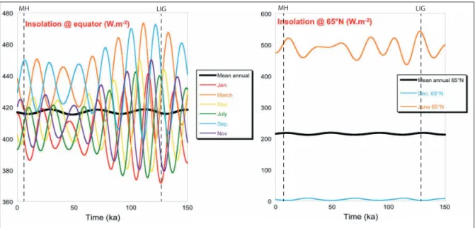
Comparing climate simulations for the LIG (dated at ~127 ka) and the MH (dated at 6 ka) is ideal to better understand the impact of orbital forcing on the global climate state, when atmospheric CO2 concentrations and continental configuration were similar to those observed under pre-industrial climatic background conditions (Otto-Bliesner et al., 2016). At low latitudes insolation is high year-round, yet the precession of the equinoxes induces substantial long-term insolation changes for a given month, with out-of-phase insolation changes for months that are opposite within the annual cycle (such as March and September, fig. 2). At high latitudes, seasonal insolation changes are massive, ranging from very low values in winter to values surpassing those recorded at the equator for June (fig. 2). The long-term (multi-millen-nial) changes in seasonal insolation will also be twice as large for the LIG compared to the MH period because the magnitude of the precessional forcing is shaped by eccentricity, which was much larger during the LIG than the Holocene (fig. 2). Mean-annual insolation changes at a given latitude are solely induced by obliquity, and are negligible when compared to seasonal insolation changes induced by precession (fig. 2). This implies that any record that contains variability at the precessional periods – potentially including some SST records for the Holocene and the Last Interglacial period – must be skewed towards certain months of the year (Huybers &
Wunsch, 2003). This could have important implications when comparing different SST records skewed towards contrasting seasons.
The LIG is a period during which global temperatures are thought to have been warmer than preindustrial tempe-ratures by ~1°C (Dutton et al., 2015). The LIG PMIP expe-riments target the 127 ± 1 ka time slice, corresponding to a time window during which the orbital configuration led to maximum insolation at northern high latitudes during the summer solstice (fig. 2). Such a precise time slice implies that the main source of uncertainties in model-data comparison will depend on the precision and the accuracy of the age model of individual SST records (see Govin et
al., 2015 for a review). The available SST databases for
the LIG are not yet able to provide age models that meet these quality requirements, since they either integrate SST anomalies over long (multi-millennial) time periods, or target the LIG peak warmth (Turney & Jones, 2010; McKay et al., 2013; Past Interglacials Working Group of PAGES, 2016). A set of high-resolution SST records for the LIG with refined age models has been published by Capron et al. (2014), but was focused on high-latitude sites exclusively. The construction of a global LIG SST database for the 127 ka time slice is underway, however, and will allow model-data comparisons with minimal age uncertainties (Capron et al., submitted).
The mid-Holocene (MH) is another period thought to have been warmer than the pre-industrial background climate by ~0.5°C (Marcott et al., 2013), and is docu-mented by a wealth of well-dated SST records. Such abundance in high-quality marine records theoretically makes this time interval easier to study than the LIG. However, the reported SST anomalies during the MH are often smaller than those reported for the LIG (see e.g. Leduc et al., 2010a), which given the proxy
uncer-MH LIG MH LIG
Figure 2: Changes in insolation forcing at the equator (left panel) and at 65°N (right panel) over the last 150 ka for some selected months of the year (data from Laskar, 2004).
Dotted lines indicate the 6 and 127 ka time slices targeted for the MH and the LIG model simulations, respectively (see text for details). Note that the effect of daylight duration at high latitudes surpasses that of the angle of incoming solar radiation to explain higher insolation values at high latitudes as compared to the equator in June.
Figure 2 : Changements d’insolation à l’équateur (panneau de gauche) et à 65°N (panneau de droite) sur les 150 derniers ka pour une sélection de certains mois de l’année (d’après Laskar, 2004). Les lignes pointillées repèrent les intervalles à 6 et 127 ka ciblés pour les simulations du MH et du LIG, respectivement (voir le texte pour plus de détails). Il est à noter que l’effet de la longueur de l’ensoleillement journalier à 65°N explique les valeurs d’insolation plus élevées à ces latitudes par rapport à celles reportées pour l’équateur au mois de juin.
tainties makes this time interval harder to study than the LIG. An overview of the uncertainties associated with SST anomalies for the MH indicates that the metho-dological uncertainties are indeed often larger than the reported climate anomalies themselves, suggesting that a precise and accurate model-data comparison is difficult to achieve (Hessler et al., 2014).
For both interglacials, further evaluations of depth habitat and/or seasonal artifacts that may contribute to biases in the SST reconstructions are warranted. It is, however, extremely challenging to assign one SST proxy to a specific season since proxy sensitivity changes from one region to another. Schneider et al. (2010) combined satellite data for monthly changes in SST and primary productivity – the latter was assumed to reflect cocco-lithophorid productivity and used to infer seasonal changes in alkenone synthesis on a global scale. They defined a seasonality index to map the relationship between seasonal changes in SST and productivity for the global ocean (Schneider et al., 2010). At high latitudes, the seasonality index is positive, reflecting the fact that
photosynthesizing organisms such as coccolithophorids usually thrive during summer, when both insolation and SSTs reach their maximum (Bijma, 2000; Schneider
et al., 2010). At low latitudes, where the open-ocean is
permanently stratified and solar irradiance is high year-round, surface nutrients that limit phytoplankton growth are mostly replenished in the photic zone during winter, when mixing of the surface ocean increases (Behrenfeld
et al., 2006). Here, the seasonality index is negative, i.e.
productivity tends to be greatest during months when SST is below the mean-annual SST (Schneider et al., 2010).
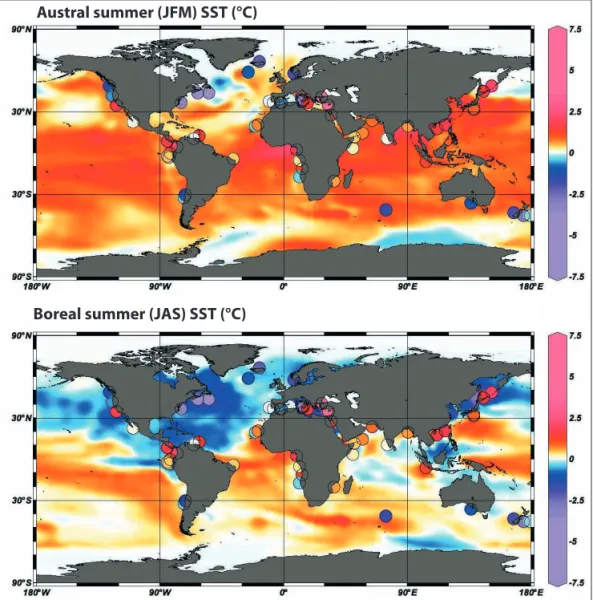
At first order, changes in Holocene SST relative to modern as estimated from alkenones suggest Holocene warming and cooling trends at low and high latitudes, respectively (Kim et al., 2004; Leduc et al., 2010a; fig. 3). Such a pattern is not captured by climate models used in the PMIP simulations of the MH (Lohmann et al., 2013). Following the global pattern of the above-described seasonality index, modelled Holocene SST trends can be reconciled with alkenone records in the northern hemis-phere when high and low latitude records are assumed to
Boreal summer (JAS) SST (°C) Austral summer (JFM) SST (°C)
Figure 3: Model-data comparison of Holocene SST trends as simulated by the Kiel Climate Model for two different seasons (coloured map, Schneider et al., 2010) and reconstructed using alkenone-based SST records (coloured dots, Leduc et al., 2010).
SST anomalies are presented as the SST difference between the early Holocene (i.e. a 9.5 ka time slice simulation for the Kiel Climate Model and the 10 +/- 1ka alkenone data) and modern (core top) simulated (estimated) SST value. fig. reproduced using the data presented in Schneider et al. (2010).
Figure 3 : Comparaison modèles - données des changements de SST pendant l’Holocène tels qu’il sont simulés par le modèle climatique de Kiel pour deux saisons différentes (carte colorée, Schneider et al., 2010) et reconstruits à l’aide des enregistrements de SST à partir des alkenones (points colorés, Leduc et al., 2010). Les anomalies de SST reportées représentent la différence de SST entre l’Holocène précoce (centrée sur 9,5 ka pour le modèle climatique de Kiel et les données d’alkenone datées à 10 +/- 1ka) et la valeur de SST simulée (estimée) pour la période préindustrielle (pour les valeurs de SST estimées pour le dernier millénaire). La fig. reproduit les résultats présentés dans Schneider et al. (2010).
reflect boreal summer and winter, respectively (Schneider
et al., 2010; Lohmann et al., 2013; fig. 3). This suggests
that accounting for the basic ecological requirements of primary producers such as coccolithophorids in model-data comparisons holds the key to reducing at least parts of the model-data mismatches for the MH.
While alkenone-based MH records generally do not agree with Mg/Ca-based records, potentially because the relevant organisms thrive during different seasons and/or record different water depths, Holocene records of SST based on Mg/Ca and TEX86 generally agree with each other, suggesting that the emerging TEX86 proxy can help to fill gaps in MH databases (Hertzberg et al., 2016). TEX86 can be particularly useful in locations where Mg/Ca and alkenones cannot be easily applied, such as in the Southern Ocean (Ho et al., 2014), here again with a strong summer bias (Shevenell et al., 2011). Yet, the coherence between TEX86 and Mg/Ca Holocene SST estimates does not always hold beyond the Holocene time window since it may be overprinted by a subsurface signal (Hertzberg et al., 2016), challenging the applica-bility of the TEX86 SST proxy under climate backgrounds that are fundamentally different such as the LGM.
A comparison of Holocene and LIG SST trends as estimated from alkenones and Mg/Ca indicates that SST trends are generally of the same sign, but with larger magnitudes estimated for the LIG compared to the Holo-cene (Leduc et al., 2010a, fig. 4). Those SST trends match the magnitude and sign of the hypothesized orbital forcing relevant for the individual records (Leduc et al., 2010a, fig. 4). It is worth noting that modern fluxes of alkenones to the seafloor, based on measurements of export using sediment traps, are generally inconsistent with the
seaso-nality index presented in Schneider et al. (2010) based on satellite estimations of primary productivity (see e.g. Rosell-Mélé & Prahl, 2013; Richey & Tierney, 2016), and this conundrum still needs to be resolved. Given that the modern annual range of SST is greater than the reported MH SST anomaly in many regions (fig. 1 and 3), and considering that mixed layer temperature lags the orbi-tally-induced changes of the shortwave radiation forcing by several months (Timmermann et al., 2013), it is crucial for the study of interglacials to consider the seasonality embedded in each proxy since many of them – if not all – are likely skewed towards some particular season.
3.3 - THE LAST GLACIAL MAXIMUM AND THE LAST DEGLACIATION
The Last Glacial Maximum (LGM), by definition, is the last time when continental ice sheets reached their maximum volume, and eustatic sea level subsequently reached a low stand (EPILOG, 2001; Clark et al., 2009). The EPILOG project (Environmental Processes of the Ice age: Land, Oceans, Glaciers) defined the LGM time window as the 19-23 ka time interval (EPILOG, 2001). Even though more recent eustatic sea level reconstruc-tions document an earlier onset of the glacial maximum dated at 30 ka (Lambeck, 2014), PMIP experiments use boundary conditions as defined for 21 ka (Braconnot, 2007). The LGM time interval is immediately followed by the onset of the last deglaciation, which runs through the entire 21-9 ka time interval in the PMIP4 experi-mental design (Ivanovic et al., 2016). Modelling this 11 kyr-long time window allows us to study climate variability under constantly changing boundary
condi-10 12 14 16 18 20 22 24 116 118 120 122 124 126 128 130 0 2 4 6 8 10 12 14 A lk e n o n e -der iv ed SST (° C) 116 118 120 122 124 126 128 130 Age (kyr BP) 0 2 4 6 8 Age (kyr BP) Insolation changes (W .m-2) 440 460 480 500 520 540 Age (kyr BP) 22 23 24 25 26 27 28 0 2 4 6 8 116 118 120 122 124 126 128 130 Age (kyr BP) Age (kyr BP) A lk e n o n e -der iv ed SST (° C) 370 390 410 430 450 0 2 4 6 8 Age (kyr BP) Insolation changes (W .m-2) 116 118 120 122 124 126 128 130 370 390 410 430 450 0 2 4 6 8 Age (kyr BP) Insolation changes (W .m-2) 116 118 120 122 124 126 128 130 27 28 29 30 31 32 0 2 4 6 8 116 118 120 122 124 126 128 130 Age (kyr BP) Age (kyr BP) Mg /C a -der iv ed SST (° C) Martrat et al. (2007)
Herbert and Schuffert (2000) Visser et al. (2003)
July, 35°N
January, 0°N July, 0°N
10 12 14
10 12 14
10 12 14 10 12 14 10 12 14
Cariaco Basin (Caribbean Sea), alkenones Indonesian archipelago (Mg/Ca) Western Mediterranean Sea (Alkenones)
Figure 4: Comparison of SST trends for the Holocene and the last interglacial period for some selected regions and proxies (Leduc et al., 2010).
Figure 4 : Comparaison des changements de SST reconstruits pour l’Holocène et pour la dernière période interglaciaire pour certaines régions et proxys sélectionnés (Leduc et al., 2010).
tions, including the severe climate changes that occurred at the millennial timescale associated with North Atlantic fresh water fluxes (Ivanovic et al., 2016).
The most recent extensive SST database available for the LGM is the MARGO database (MARGO, 2009). Since the publication of this database, model-data comparisons have used it to constrain climate sensitivity (Schmittner
et al., 2011; Hargreaves et al., 2012). The MARGO
data-base reports much more heterogeneous SST results than climate model simulations (Kageyama et al., 2013), in particular in the tropics. Such heterogeneity may in part be embedded in the multitude of proxy types employed to reconstruct LGM SST. That aspect was addressed in the framework of the initial results of the COMPARE working group, that reported tropical SST cooling of 2°C for alkenone-based SST vs. a 3°C cooling estimated with Mg/Ca (Lea et al., 2014). After substantial incorporation of high-quality records and a thorough data quality-control exercise, the Sensitivity of the Tropics (SENSETROP) working group has refined the LGM cooling for low latitudes, and reported comparable SST cooling of - 2.3 ± 0.8 °C and - 2.4 ± 0.8 °C for alkenone and Mg/ Ca-based SST records, respectively (de Garidel-Thoron et al, 2016; Lea et al., 2016). In contrast to alkenone and Mg/Ca results, tropical SST anomalies for the LGM based on the TEX86 paleothermometer are much larger, suggesting that it is representative of deep subsurface water temperature (Lopes dos Santos et al., 2010; Ho & Laepple, 2015; Hertzberg et al., 2016). Thus, although combining TEX86 with other SST proxies might help track changes in water column stratification (see e.g. Tierney
et al., 2016), its use as a SST proxy for the LGM time
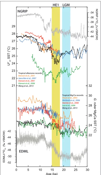
window should be avoided (Hertzberg et al., 2016). To date, the most comprehensive SST database for the last deglaciation based on geochemical proxy records is probably the one published in Shakun et al. (2012). During most of the deglaciation time interval, a succes-sion of rapid swings in temperatures, named Heinrich Event 1 (HE1, ~18-15 ka), the Bolling-Allerod (BA, ~15-13 ka) and the Younger Dryas (YD, ~13-11.7 ka), occurred in the northern hemisphere at mid and high lati-tudes (Shakun et al., 2012). The bipolar thermal seesaw is a climate mechanism associated with the efficiency with which the interhemispheric redistribution of heat takes place when the Atlantic Meridional Overturning Circu-lation (AMOC) is turned on (such as during the BA) and off (such as during the HE1 and the YD). It predicts that temperatures in the southern hemisphere will increase during cold North Atlantic spells because the collapse of the AMOC leads to temperature buildup in the southern hemisphere (Stocker & Johnsen, 2003). During the last deglaciation, the thermal seesaw is most apparent when Greenland and Antarctic ice cores temperature records are compared: while temperatures increased in Antarctica during the cold North Atlantic intervals of HE1 and the YD, Antarctic warming ceased during the warm period of the BA in Greenland (fig. 5).
While such a seesaw is clearly seen at mid to high latitudes in the ocean (Lamy et al., 2007; Shakun et al., 2012), SST changes in the tropics over the last
degla-ciation are more puzzling. It has been recognized for a decade that, in the tropics, different proxies do not track synchronous deglacial SST warming (de Garidel-Thoron
et al., 2007), with UK’37 warming generally lagging Mg/Ca
temperature records (Shakun et al., 2012). A number of processes have been put forward to explain this complex response. It was first suggested that differences in the water depth habitat of planktonic foraminifera and cocco-lithophores combined to calcite dissolution changes could be responsible for this mismatch (de Garidel-Thoron et al., 2007). As the number of available records of Mg/Ca and alkenone-based SST for sites located close to the equator increased, it became apparent that many alkenone records mimic the temperature evolution seen in the northern hemisphere. On the other hand, Mg/Ca records, including sites where dissolution did not impact foraminiferal Mg/Ca, mimic the warming sequence observed in the southern hemisphere (Kiefer & Kienast, 2005 ; Wang et al., 2013, fig. 5), with the exception of the Arabian Sea (Tierney et al., 2016). The effect of seaso-nality has been proposed to account for this deglacial equatorial pattern: for those regions where the Intertro-pical Convergence Zone (ITCZ) passes overhead twice a year, a marine core location could be under the alternate influence of climate variability in both the northern and southern hemispheres, given that the ITCZ represents the meteorological equator (Wang et al., 2013). In this case, if different proxies are sensitive to different seasons, multiple proxies could theoretically track temperatures under seasonal situations sensitive to the northern or the southern hemisphere. Model-data comparison of equato-rial Pacific sites highlighted that model-data matching is achieved only when alkenones – that mimic Greenland temperatures – are compared to modelled boreal winter SSTs, and Mg/Ca – that mimic Antarctic temperatures – are compared to boreal summer SSTs (Timmermann et
al., 2014). It is also likely that contrasting water depth
habitats of different Globigerinoides ruber morphotypes mixed in the same Mg/Ca record might also blur the deglacial hydrological structure changes (Steinke et al., 2001; Regoli et al., 2015). It would imply that surface and subsurface temperatures are not sensitive to the same hemisphere. The proxy-dependent dynamics of the degla-ciation are likely a combination of the different processes highlighted here: in the Shakun et al. (2012) database, within the tropical latitudinal band, 21 out of 36 SST records are based on Mg/Ca, suggesting that the overall warming of the tropics reconstructed during HE1 and the YD in the northern hemisphere could at least partly be an artifact of the over-representation of Mg/Ca relative to alkenone records in the database. Regardless of the exact timing of SST changes during the last deglaciation, the reasons why alkenone- and Mg/Ca-based data are not in phase is a conundrum that still needs to be resolved. 3.4 - THE LAST MILLENNIUM
Model experiments focused on the last millennium (i.e. the 850-1850 years of the Common Era (CE), as defined in Jungclaus et al., 2016) aim to study natural climate
varia-bility on decadal to millennial timescales. The last millen-nium period encompasses two periods often referred to as the “Medieval Climate Anomaly” (MCA) and the “Little Ice Age” (LIA), that have recently been extensively docu-mented in the framework of the PAGES2k group (see PAGES2k, 2013; McGregor et al., 2015 among others). Although the exact subdivision of those two periods is often vaguely defined in the literature, there is increasing evidence that the first part of the MCA was particularly stable because of the lack of important changes in natural
climate forcing until ~1025 CE (Bradley et al., 2016). Similarly to the MCA, the LIA time window is often not clearly defined, but the recent literature tends to date the beginning of the LIA to the mid 13th century when a series
of clustered explosive volcanic eruptions and solar irra-diance minima led to a departure from the previous unper-turbed climate forcing factors (note that the PAGES2k consortium labeled the continental temperature cooling periods that started in the mid-1250s as being triggered by “volcanic-solar turndowns”, PAGES2k, 2013).
LGM HE1 NGRIP
EDML
Tropical alkenone records:
Kienast et al., 2001
Jaeschke et al., 2007 Kienast et al., 2001 Kienast et al., 2006 Wang et al., 2013
Tropical Mg/Ca records:
Visser et al., 2003
Weldeab et al., 2006 Steinke et al., 2008 Lea et al., 2006 Wang et al., 2013
Figure 5: Upper curves: comparison of a selection of alkenone records compared to Greenland (NORTHGRIP, 2004) temperatures. Lower panels: comparison of a selection of Mg/Ca records compared to Antarctic temperatures (EPICA, 2006).
SST records are coloured in green for the eastern equatorial Pacific sites, in blue for the western equatorial Atlantic sites, in black for the western tropical Indian Ocean (Mozambique channel) site, and red and yellow for the Indonesian archipelago. Blue and green vertical bars indicate the LGM and HE1 chronozone, respectively. Note the contrast of alkenones and Mg/Ca SST changes that either increase rapidly at the end of the HE1 or decrease progressively during the full HE1 chronozone, respectively, as predicted by the interhemispheric thermal seesaw model of Stocker and Johnsen (2003).
Figure 5 : Courbes supérieures: comparaison entre une sélection d’enregistrements d’alkenone aux températures du Groënland (NORTHGRIP, 2004). Panneaux inférieurs: comparaison d’une sélection d’enregistrements de Mg/Ca par rapport aux températures antarctiques (EPICA, 2006). Les enre-gistrements en vert proviennent du Pacifique Est-équatorial, en bleu de l’Atlantique Ouest-équatorial, en noir de l’océan Indien Ouest-tropical (canal du Mozambique) et rouge en et jaune l’archipel indonésien. Les barres verticales bleues et vertes indiquent respectivement les périodes du dernier maximum glaciaire et l’évènement Heinrich 1 (HE1). Notons le contraste des changements de SST estimés avec les alkenones et le Mg/Ca qui, respec-tivement, augmentent rapidement à la fin du HE1 et décroissent progressivement pendant le HE1, à l’image du modèle de balançoire thermique inte-rhémisphérique de Stocker et Johnsen (2003).
In marine sediments, available high-quality SST data have clearly detected the onset of a cooling acceleration associated with the LIA (McGregor et al., 2015). Yet, various technical difficulties associated with geoche-mical proxies hinder the precise and accurate detection in space and time of this onset in individual SST records (McGregor et al., 2015). First, marine sequences are particularly difficult to precisely date for the last millen-nium, and contrarily to other types of archives commonly used to study the recent past – such as corals or tree rings – it is almost impossible to achieve annual resolu-tion because bioturbaresolu-tion acts to smooth the sedimentary signal. Second, the magnitude of SST changes over the last millennium is often within the range of the proxy uncertainty, which makes it challenging to infer signi-ficant changes in SST. Third, sediment retrieval during coring is imperfect, and the uppermost sediment layer is often missing. Ideally, a combination of long cores and shorter multicores taken at the same site would be used, to preserve the marine-sediment interface and ensure proper recovery of the uppermost few centimeters of the sedimentary sequence.
Yet despite these problems, when all proxies are collated into a single standardized SST record hypothe-sized to be representative of the global ocean, a signi-ficant cooling acceleration associated with the onset of the LIA can be extracted from standardized SST data (McGregor et al., 2015). Interestingly, the sign of SST change does not seem to depend on whether alkenones, Mg/Ca or TEX86 were employed to estimate SST, unlike what was recognized earlier for the Holocene period (McGregor et al., 2015). During the Holocene, the largest forcing at play for explaining SST trends is probably orbital forcing, which has opposite signs of change for opposite seasons at a given location. If, as suggested by McGregor et al. (2015), the clustering of explosive volcanic eruptions is the most likely first-order forcing factor for the LIA cooling, the nature of the forcing itself might explain why all types of SST proxies respond in the same manner. During volcanic eruptions, and despite significant warming that occurs in the northern hemis-phere during the winter immediately following the largest tropical eruptions, the net impact of the aerosol atmospheric loading following large eruptions is a global cooling that could last several years, independent of the season and/or the hemisphere (Zanchettin et al., 2016). This may explain why collating and aggregating different kinds of geochemical proxies that are sensitive to contras-ting seasons and/or marine environment types may not be as problematic as for other periods over which different climate forcing factors drive variability.
4 - CONCLUSIONS
Geochemical proxies for SST such as the UK’37, the
Mg/Ca and the TEX86 paleothermometers are now rela-tively well-established paleoclimate tools, however, it should be kept in mind that refining the understan-ding of these SST proxies is an ongoing process that
involves a large community in the field of paleoceano-graphy and proxy refinement. SST databases, which are built, quality-controlled and provided to the mode-ling community by paleoceanographers, should not be seen as static tools. They must be compared to SST model outputs with some basic understanding of the processes behind how proxies record and integrate the SST signals in a given location. In particular, geoche-mical SST proxies should be interpreted through the prism of the carrier organisms’ ecology, as well as other sources of uncertainty such as oceanic and sedimen-tary mixing processes. Statistical models accounting for those processes can achieve significant advances in interpreting proxy discrepancies (Laepple & Huybers, 2013; Ho & Laepple, 2016). In such a way, it might be feasible to go a step further towards better understan-ding why models do not reproduce SST as estimated from geochemical proxies, providing further room for evaluating and calibrating climate models outside of the historical period (Braconnot et al., 2012; Laepple & Huybers, 2014).
ACKNOWLEDGEMENTS
We thank Emilie Capron for discussion on the uncer-tainties associated with LIG SST databases and Frank Bassinot for his careful reading and useful suggestions on an earlier version of the manuscript.
REFERENCES
ABRAM N.J., McGREGOR H.V., TIERNEY J.E., EVANS M.N., McKay N.P., KAUFMAN D.S., THIRUMALAI K., & THE PAGES2k CONSORTIUM, 2016 - Early onset of industrial-era warming across the oceans and continents, Early onset of industrial-era warming across the oceans and continents. Nature, 536, 411-418. ANAND P., ELDERFIELD H. & CONTE M.H., 2003 - Cali-bration of Mg/Ca thermometry in planktonic foraminifera from a sediment trap time series. Paleoceanography, 18 (2), 1050, doi:10.1029/2002PA000846.
ANDRULEIT H., STÄGER S.U. & CEPEK P., 2003 - Living cocco-lithophores in the northern Arabian Sea: ecological tolerances and environmental control. Marine Micropaleontology, 49 (1), 157-181. ARBUSZEWSKI J., DeMENOCAL P., KAPLAN A. & FARMER
E.C., 2010 - On the fidelity of shell-derived delta O-18(seawater) estimates. Earth and Planetary Science Letters, 300, 185-196. BARD E., 2001 - Comparison of alkenone estimates with other
paleo-temperature proxies. Geochemistry, Geophysics Geosystems, 2, 1002, doi:10.1029/2000GC000050.
BARKER S., GREAVES M. & ELDERFIELD H., 2003 - A study of cleaning procedures used for foraminiferal Mg/Ca paleother-mometry. Geochemistry, Geophysics Geosystems, 4(9), 8407, doi:10.1029/2003GC000559.
BEAUFORT L., COUAPEL M., BUCHET N., CLAUSTRE H. & GOYET C., 2008 - Calcite production by coccolithophores in the south east Pacific Ocean. Biogeosciences, 5, 1101-1117.
BEHRENFELD M.J., O’MALLEY R., SIEGEL D., McCLAIN C., SARMIENTO J., FELDMAN G., MILLIGAN A., FALKOWSKI P., LETELLIER R. & BOSS E., 2006 - Climate-driven trends in contemporary ocean productivity. Nature, 444, 752-755.
BENDER M.L., LORENS R.B. & WILLIAMS F.D., 1975 - Sodium, magnesium and strontium in the tests of planktonic foraminifera.
Micropaleontology, 21, 448-459.
BENTHIEN A. & MÜLLER P.J., 2000 - Anomalously low alkenone temperatures caused by lateral particle and sediment transport in the Malvinas Current region, western Argentine Basin. Deep-Sea